
Divergence and Sufficiency for Convex Optimization

GSK Department, Copenhagen Business College, Nørre Voldgade 34, 1358 Copenhagen K, Denmark
Entropy 2017, 19(5), 206; https://doi.org/10.3390/e19050206
Submission received: 30 December 2016
/
Revised: 11 April 2017
/
Accepted: 2 May 2017
/
Published: 3 May 2017
(This article belongs to the Special Issue Convex Optimization and Entropy)
Abstract
:Logarithmic score and information divergence appear in information theory, statistics, statistical mechanics, and portfolio theory. We demonstrate that all these topics involve some kind of optimization that leads directly to regret functions and such regret functions are often given by Bregman divergences. If a regret function also fulfills a sufficiency condition it must be proportional to information divergence. We will demonstrate that sufficiency is equivalent to the apparently weaker notion of locality and it is also equivalent to the apparently stronger notion of monotonicity. These sufficiency conditions have quite different relevance in the different areas of application, and often they are not fulfilled. Therefore sufficiency conditions can be used to explain when results from one area can be transferred directly to another and when one will experience differences.
Keywords:
Bregman divergence; entropy; exergy; Kraft’s inequality; locallity; monotonicity; portfolio; regret; scoring rule; sufficiency1. Introduction
One of the main purposes of information theory is to compress data so that data can be recovered exactly or approximately. One of the most important quantities was called entropy because it is calculated according to a formula that mimics the calculation of entropy in statistical mechanics. Another key concept in information theory is information divergence (KL-divergence) that is defined for probability vectors P and Q as
It was introduced by Kullback and Leibler in 1951 in a paper entitled On Information and Sufficiency [1]. The link from information theory back to statistical physics was developed by E.T. Jaynes via the maximum entropy principle [2,3,4]. The link back to statistics is now well established [5,6,7,8,9].
Related quantities appear in information theory, statistics, statistical mechanics, and finance, and we are interested in a theory that describes when these relations are exact and when they just work by analogy. First we introduce some general results about optimization on state spaces of finite dimensional C*-algebras. This part applies exactly to all the topics under consideration and lead to Bregman divergences or more general regret functions. Secondly, we introduce several notions of sufficiency and show that this leads to information divergence. In a number of cases it is not possible or not relevant to impose the condition of sufficiency, which can explain why regret function are not always equal to information divergence.
2. Structure of the State Space
Our knowledge about a system will be represented by a state space. I many applications the state space is given by a set of probability distributions on a sample space. In such cases the state space is a simplex, but it is well-known that the state space is not a simplex in quantum physics. For applications in quantum physics the state space is often represented by a set of density matrices, i.e., positive semidefinite complex matrices with trace 1. In some cases the states are represented as elements of a finite dimensional -algebra, which is a direct sum of matrix algebras. A finite dimensional -algebra that is a sum of matrices has a state space that is a simplex, so the state spaces of finite dimensional -algebras contain the classical probability distributions as special cases.
The extreme points in the set of states are the pure states. The pure states of a -algebra can be identified with projections of rank 1. Two density matrices and are said to be orthogonal if Any state s has a decomposition
where are orthogonal pure states. Such a decomposition is not unique, but for a finite dimensional -algebra the coefficients are unique and are called the spectrum of the state.
Sometimes more general state spaces are of interest. In generalized probabilistic theories a state space is a convex set where mixtures are defined by randomly choosing certain states with certain probabilities [10,11]. A convex set where all orthogonal decompositions of a state have the same spectrum, is called a spectral state space. Much of the theory in this paper can be generalized to spectral sets. The most important spectral sets are sets of positive elements with trace 1 in Jordan algebras. The study of Jordan algebras and other spectral sets is relevant for the foundation of quantum theory [12,13,14,15], but in this paper we will restrict our attention to states on finite dimensional -algebras. Nevertheless some of the theorems and proofs are stated in such a way that they hold for more general state spaces.
3. Optimization
Let denote a state space of a finite dimensional -algebra and let denote a set of self-adjoint operators. Each is identified with a real valued measurement. The elements of may represent feasible actions (decisions) that lead to a payoff like the score of a statistical decision, the energy extracted by a certain interaction with the system, (minus) the length of a codeword of the next encoded input letter using a specific code book, or the revenue of using a certain portfolio. For each the mean value of the measurement is given by
In this way the set of actions may be identified with a subset of the dual space of .
Next we define
We note that F is convex, but F need not be strictly convex. In principle may be infinite, but we will assume that for all states s. We also note that F is lower semi-continuous. In this paper we will assume that the function F is continuous. The assumption that F is a real valued continuous function is fulfilled for all the applications we consider.
If s is a state and is an action then we say that a is optimal for s if . A sequence of actions is said to be asymptotically optimal for the state s if for
If are actions and is a probability vector then we we may define the mixed action as the action where we do the action with probability We note that We will assume that all such mixtures of feasible actions are also feasible. If almost surely for all states we say that dominates and if almost surely for all states s we say that strictly dominates All actions that are dominated may be removed from without changing the function Let denote the set of self-adjoint operators (observables) a such that Then Therefore we may replace by without changing the optimization problem.
In the definition of regret we follow Servage [16] but with different notation.
Definition 1.
Let F denote a convex function on the state space . If is finite the regret of the action a is defined by
The notion of regret has been discussed in detail in [17,18,19]. In [20] it was proved that if a regret based decision procedure is transitive then it must be equal to a difference in expected utility as in Equation (1), which rules out certain non-linear models in [17,19].
Proposition 1.
The regret of actions has the following properties:
- with equality if a is optimal for s.
- is a convex function.
- If is optimal for the state where is a probability vector then
- is minimal if a is optimal for .
If the state is but one acts as if the state were one may compare what one achieves and what could have been achieved. If the state has a unique optimal action a we may simply define the regret of by
The following definition leads to a regret function that is essentially equivalent to the so-called generalized Bregman divergences defined by Kiwiel [21,22].
Definition 2.
Let F denote a convex function on the state space . If is finite then we define the regret of the state as
where the infimum is taken over all sequences of actions that are asymptotically optimal for
With this definition the regret is always defined with values in and the value of the regret only depends on the restriction of the function F to the line segment from to . Let f denote the function where . As illustrated in Figure 1 we have
where denotes the right derivative of f at . Equation (2) is even valid when the regret is infinite if we allow the right derivative to take the value −∞.
If the state has the unique optimal action then
so the function F can be reconstructed from except for an affine function of The following proposition follows from Alexandrov’s theorem ([23], Theorem 25.5).
Proposition 2.
A convex function on a finite dimensional convex set is differentiable almost everywhere with respect to the Lebesgue measure.
A state where F is differentiable has a unique optimal action. Therefore Equation (3) holds for almost any state . In particular the function F can be reconstructed from except for an affine function.
Proposition 3.
The regret of states has the following properties:
- with equality if there exists an action a that is optimal for both and .
- is a convex function.
Further, the following two conditions are equivalent:
- implies .
- The function F is strictly convex.
We say that a regret function is strict if F is strictly convex. The two last properties Proposition 1 do not carry over to regret for states except if the regret is a Bregman divergence as defined below. The regret is called a Bregman divergence if it can be written in the following form
where denotes the (Hilbert-Schmidt) inner product. In the context of forecasting and statistical scoring rules the use of Bregman divergences dates back to [24]. A similar but less general definition of regret was given by Rao and Nayak [25] where the name cross entropy was proposed. Although Bregman divergences have been known for many years they did not gain popularity before the paper [26] where a systematic study of Bregman divergences was presented.
We note that if is a Bregman divergence and minimizes F then so that the formula for the Bregman divergence reduces to
Bregman divergences satisfy the Bregman identity
but if F is not differentiable this identity can be violated.
Example 1.
Let the state space be the interval with two actions and Let and Let further and Then If then
but
The following proposition is easily proved.
Proposition 4.
For a convex and continuous function F on the state space the following conditions are equivalent:
- The function F is differentiable in the interior of any face of .
- The regret is a Bregman divergence.
- The Bregman identity (5) is always satisfied.
- For any probability vectors the sum is always minimal when .
4. Examples
In this section we shall see how regret functions are defined in some applications.
4.1. Information Theory
We recall that a code is uniquely decodable if any finite sequence of input symbols give a unique sequence of output symbols. It is well-known that a uniquely decodable code satisfies Kraft’s inequality (see [27] and ([28], Theorem 3.8))
where denotes the length of the codeword corresponding to the input symbol and denotes the size of the output alphabet . Here the length of a codeword is an integer. If is a probability vector over the input alphabet, then the mean code-length is
Our goal is to minimize the expected code-length. Here the state space consist of probability distributions over the input alphabet and the actions are code-length functions.
Shannon established the inequality
It is a combinatoric problem to find the optimal code-length function. In the simplest case with a binary output alphabet the optimal code-length function is determined by the Huffmann algorithm.
A code-length function dominates another code-length function if all letters have shorter code-length. If a code-length function is not dominated by another code-length function then for all the length is bounded by For fixed alphabets and there exists only a finite number of code-length functions ℓ that satisfy Kraft’s inequality and are not dominated by other code-length functions that satisfying Kraft’s inequality.
4.2. Scoring Rules
The use of scoring rules has a long history in statistics. An early contribution was the idea of minimizing the sum of square deviations that dates back to Gauss and works perfectly for Gaussian distributions. In the 1920s, Ramsay and de Finetti proved versions of the Dutch book theorem where determination of probability distributions were considered as dual problems of maximizing a payoff function [29]. Later it was proved that any consistent inference procedure corresponds to optimizing with respect to some payoff function. A more systematic study of scoring rules was given by McCarthy [30].
Consider an experiment with as sample space. A scoring rule f is defined as a function such that the score is when a prediction has been given in terms of a probability distribution Q and has been observed. A scoring rule is proper if for any probability measure the score is minimal when Here the state space consist of probability distributions over and the actions are predictions over , which are also probability distributions over .
There is a correspondence between proper scoring rules and Bregman divergences as explained in [31,32]. If is a Bregman divergence and g is a function with domain then f given by defines a scoring rule.
Assume that f is a proper scoring function. Then a function F can be defined as
This lead to the regret function
Since f is assumed to be proper . The Bregman identity (5) follows by straight forward calculations. With these two results we see that the regret function is a Bregman divergence and that
Hence a proper scoring rule f has the form where . A strictly proper scoring rule can be defined as a proper scoring rule where the corresponding Bregman divergence is strict.
Example 2.
The Brier score is given by
The Brier score is generated by the strictly convex function .
4.3. Statistical Mechanics
Thermodynamics is the study of concepts like heat, temperature and energy. A major objective is to extract as much energy from a system as possible. The idea in statistical mechanics is to view the macroscopic behavior of a thermodynamic system as a statistical consequence of the interaction between a lot of microscopic components where the interacting between the components are governed by very simple laws. Here the central limit theorem and large deviation theory play a major role. One of the main achievements is the formula for entropy as a logarithm of a probability.
Here we shall restrict the discussion to the most simple kind of thermodynamic system from which we want to extract energy. We may think of a system of non-interacting spin particles in a magnetic field. For such a system the Hamiltonian is given by
where is the spin configuration, is the magnetic moment, is the strength of an external magnetic field, and is the spin of the the j’th particle. If the system is in thermodynamic equilibrium the configuration probability is
where is the partition function
Here is the inverse temperature of the spin system and is Boltzmann’s constant.
The mean energy is given by
which will be identified with the internal energy U defined in thermodynamics. The Shannon entropy can be calculated as
The Shannon entropy times k will be identified with the thermodynamic entropy S.
The amount of energy that can be extracted from the system if a heat bath is available, is called the exergy [33]. We assume that the heat bath has temperature and the internal energy and entropy of the system are and if the system has been brought in equilibrium with the heat bath. The exergy can be calculated by
The information divergence between the actual state and the corresponding state that is in equilibrium with the environment is
Hence
This equation appeared already in [34].
4.4. Portfolio Theory
The relation between information theory and gambling was established by J. L. Kelly [35]. Logarithmic terms appear because we are interested in the exponent in the exponential growth rate of our wealth. Later Kelly’s approach has been generalized to trading of stocks although the relation to information theory is weaker [36].
Let denote price relatives for a list of k assets. For instance means that 5-th asset increases its value by 4%. Such price relatives are mapped into a price relative vector
Example 3.
A special asset is the safe asset where the price relative is 1 for any possible price relative vector. Investing in this asset corresponds to placing the money at a safe place with interest rate equal to 0%.
A portfolio is a probability vector where for instance means that 30% of the money is invested in asset no. 5. We note that a portfolio may be traded just like the original assets. The price relative for the portfolio is The original assets may be considered as extreme points in the set of portfolios. If an asset has the property that the price relative is only positive for one of the possible price relative vectors, then we may call it a gambling asset.
We now consider a situation where the assets are traded once every day. For a sequence of price relative vectors and a constant re-balancing portfolio the wealth after n days is
where the expectation is taken with respect to the empirical distribution of the price relative vectors. Here is proportional to the doubling rate and is denoted where P indicates the probability distribution of . Our goal is to maximize by choosing an appropriate portfolio The advantage of using constant rebalancing portfolios was demonstrated in [37].
Definition 3.
Let and denote two portfolios. We say that dominates if for any possible price relative vector We say that strictly dominates if for any possible price relative vector A set A of assets is said to dominate the set of assets B if any asset in B is dominated by a portfolio of assets in
The maximal doubling rate does not change if dominated assets are removed. Sometimes assets that are dominated but not strictly dominated may lead to non-uniqueness of the optimal portfolio.
Let denote a portfolio that is optimal for P and define
The regret of choosing a portfolio that is optimal for Q when the distribution is P is given by the regret function
If is not uniquely determined we take a minimum over all that are optimal for
Example 4.
Assume that the price relative vector is with probability and with probability t. Then the portfolio concentrated on the first asset is optimal for and the portfolio concentrated on the second asset is optimal for . For values of t between and the optimal portfolio invests money on both assets as illustrated in Figure 2.
Lemma 1.
If there are only two price relative vectors and the regret function is strict then either one of the assets dominates all other assets or two of the assets are orthogonal gambling assets that dominate all other assets.
Proof.
We will assume that no assets are dominated by other assets. Let
denote the two price relative vectors. Without loss of generality we may assume that
If then so that if then and the asset i is dominated by the asset Since we have assumed that no assets are dominated we may assume that
If is a probability vector over the two price relative vectors then according to [36] the portfolio is optimal if and only if
for all with equality if Assume that the portfolio is optimal. Now
is equivalent to
Similarly
is equivalent to
We have to check that
which is equivalent with
The right hand side equals the determinant
which is positive because asset j is not dominated by a portfolio based on asset and asset
We see that the portfolio concentrated in asset j is optimal for t in an interval of positive length and the regret between distributions in such an interval will be zero. In particular the regret will not be strict.
Strictness of the regret function is only possible if there are only two assets and if a portfolio concentrated on one of these assets is only optimal for a singular probability measure. According to the formulas for the end points of intervals (14) and (15) this is only possible if the assets are gambling assets. ☐
Theorem 1.
If the regret function is strict it equals information divergence, i.e.,
Proof.
If the regret function is strict then it is also strict when we restrict to two price relative vectors. Therefore any two price relative vectors are orthogonal gambling assets. If the assets are orthogonal gambling assets we get the type of gambling described by Kelly [35], for gambling equations can easily be derived [36]. ☐
5. Sufficiency Conditions
In this section we will introduce some conditions on a regret function. Under some mild conditions they turn out to be equivalent.
Theorem 2.
Let denote a regret function based on a continuous and convex function F defined on the state space of a finite dimensional -algebra. If the state space has at least three orthogonal states then the following conditions are equivalent:
- The function F equals entropy times a negative constant plus an affine function.
- The regret is proportional to information divergence.
- The regret is monotone.
- The regret satisfies sufficiency.
- The regret is local.
In the rest of this section we will describe each of these equivalent conditions and prove that they are actually equivalent. The theorems and proofs will be stated so that they hold even for more general state spaces than the ones considered in this paper.
5.1. Entropy and Information Divergence
Definition 4.
Let s denote an element in a state space. The entropy of s is defined as
where the infimum is taken over all decompositions of s into pure states .
This definition of the entropy of a state was first given by Uhlmann [38]. Using the fact that entropy is decreasing under majorization we see that the entropy of s is attained at an orthogonal decomposition [13] and we obtain the familiar equation
In general this definition of entropy does not provide a concave function on a convex set. For instance, the entropy of points in the square has local maximum in the four different points. A characterization of the convex sets with concave entropy functions is lacking.
Definition 5.
If the entropy is a concave function then the regret function is called information divergence.
The information divergence is also called Kullback–Leibler divergence, relative entropy or quantum relative entropy. In a C*-algebra we get
where Now so that
Hence
For states it reduces to the well-known formula
5.2. Monotonicity
We consider a set of maps of the state space into itself. The set will be used to represent those transformations that we are able to perform on the state space before we choose a feasible action . Let denote a map. Then the dual map maps actions into actions and is given by
Proposition 5 (The principle of lost opportunities).
If maps the set of feasible actions into itself then
Proof.
If then
because . Inequality (17) follows because ☐
Corollary 1 (Semi-monotonicity)
Let Φ denote a map of the state space into itself such that maps the set of feasible actions into itself and let denote a state that minimizes the function F. If is a Bregman divergence then
Proof.
Since minimizes F and F is differentiable we have . Since minimizes F and we also have that minimizes F and that . Therefore
which proves the inequality. ☐
Next we introduce the stronger notion of monotonicity.
Definition 6.
Let denote a regret function on the state space of a finite dimensional C*-algebra. Then is said to be monotone if
for any affine map
Proposition 6.
If a regret function based on a convex and continuous function F is monotone then it is a Bregman divergence.
Proof.
Assume that is monotone. We have to prove that F is differentiable. Since F is convex it is sufficient to prove that any restriction of F to a line segment is differentiable. Let and denote states that are the end points of a line segment. The restriction of F to the line segment is given by the convex and continuous function so we have to prove that f is differentiable.
If then according to Equation (2) we have
where denotes the derivative from the right. A dilation by a factor around decreases the regret so that
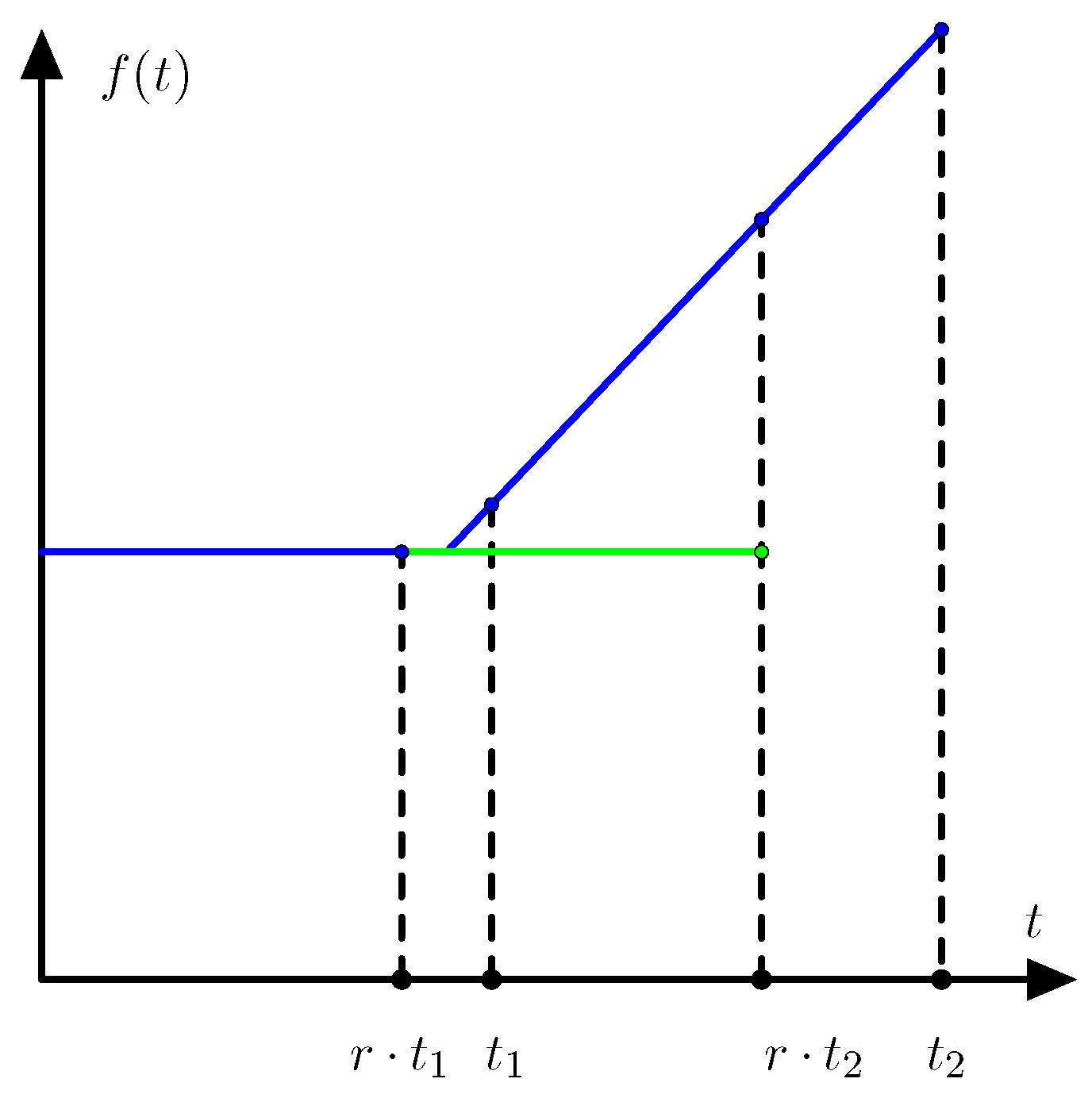
is increasing. Since f is convex the function is increasing. Assume that f is not differentiable so that has a positive jump as illustrated on Figure 3.
This contradicts that the function (19) is increasing. Therefore is continuous and f is differentiable. ☐
Recently it has been proved that information divergence on a complex Hilbert space is decreasing under positive trace preserving maps [39,40]. Previously this was only known to hold if some extra condition like complete positivity or 2-positivity was assumed [41].
Theorem 3.
Information divergence is monotone under any positive trace preserving map on the states of a finite dimensional -algebra.
Proof.
Any finite dimensional -algebra can be embedded in and there exist a conditional expectation If is a positive trace preserving map of the density matrices of into it self then is positive and trace preserving on According to Müller-Hermes and Reeb [39] we have
for density matrices in In particular this inequality holds for density matrices in and for such matrices we have . ☐
5.3. Sufficiency
The notion of sufficiency plays an important role in statistics and related fields. We shall present a definition of sufficiency that is based on [42], but there are a number of other equivalent ways of defining this concept. We refer to [43] where the notion of sufficiency is discussed in great detail.
Definition 7.
Let denote a family of states and let Φ denote an affine map where and denote state spaces. A recovery map is an affine map such that The map Φ is said to be sufficient for if Φ has a recovery map.
Proposition 7.
Assume is a regret function based on a convex and continuous function F and assume that Φ is sufficient for and with recovery map Ψ. Assume that both and map the set of feasible actions into itself. Then
Proof.
According to the principle of lest opportunities (Proposition 5) we have
Therefore Let a denote an action that is optimal for Then
and we see that is optimal for Now
where the infimum is taken over actions a that are optimal for Then
so we have The reverse inequality is proved in the same way. ☐
The notion of sufficiency as a property of divergences was introduced in [44]. The crucial idea of restricting the attention to maps of the state space into itself was introduced in [45]. It was shown in [45] that a Bregman divergence on the simplex of distributions on an alphabet that is not binary and satisfies sufficiency equals information divergence up a multiplicative factor. Here we extend the notion of sufficiency from Bregman divergences to regret functions.
Definition 8.
Let denote a regret function based on a convex and continuous function F on a state space . We say satisfies sufficiency if
for any affine map that is sufficient for
Proposition 8.
Let denote a regret function based on a convex and continuous function F on a state space . If the regret function is monotone then it satisfies sufficiency.
Proof.
Assume that the regret function is monotone. Let and denote two states and let and denote maps on the state space such that . Then
Hence ☐
Combining the previous results we get that information divergence satisfies sufficiency. Under some conditions there exists an inverse version of Proposition 8 stating that if monotonicity holds with equality then the map is sufficient. In statistics where the state space is a simplex, this result is well established. For density matrices over the complex numbers it has been proved for completely positive maps in [43]. Some new results on this topic can be found in [46].
5.4. Locality
Often it is relevant to use the following weak version of the sufficiency property.
Definition 9.
Let denote a regret function based on a convex and continuous function F on a state space . The regret function is said to be local if
when the states σ and ρ are orthogonal to and
Example 5.
On a 1-dimensional simplex (an interval) or on the Block sphere any regret function is local. The reason is that if σ and ρ are states that are orthogonal to then
Proposition 9.
Let denote a regret function based on a convex and continuous function F on a state space . If the regret function satisfies sufficiency then is local.
Proof.
Let and be states that are orthogonal to Let p denote the projection supporting the state . Let the maps and be defined by
Then and and Therefore
and
which proves the Proposition. ☐
Theorem 4.
Let be the state space of a -algebra with at least three orthogonal states, and let denote a regret function based on a convex and continuous function F on the state space . If the regret function is local then it is the Bregman divergence generated by the entropy times a negative constant.
Proof.
In the following proof we will assume that the regret function is based on the convex function First we will prove that the regret function is a Bregman divergence.
Let K denote the convex hull of a set of orthogonal states. For let denote the function . Note that is decreasing and continuous from the left. Let and where for all . If F is differentiable in P then locality implies that
Note that is a convex function and thereby it is continuous. Assume that is an arbitrary element in K and let denote a sequence such that for The sequence can be chosen so that regret is differentiable in for all Further the sequence can be chosen such that is increasing for all Then
Similarly, if the sequence can be chosen such that is increasing for all then
which implies that and that
for all j. Therefore
for all in the interior of K. In the following calculations we will assume that the distributions lie in the interior of K. The validity of the Bregman identity (5) follows directly from Equation (20) implying that is a Bregman divergence.
As a function of Q the regret is minimal when In the following calculations we write , , , and . If for then non-negativity of regret can be written as
and we note that this inequality should hold as long as Permutation of i and j leads to the inequality
that implies
where
Assume that in Inequality (21). Then
so that is mid-point convex, which for a measurable function implies convexity. Therefore is differentiable from left and right.
If and and then we have
with equality when We differentiate with respect to from right.
which is positive for so that
Since is convex we have which in combination with Inequality (23) implies that so that is differentiable. Since the function is also differentiable.
As a function of Q the Bregman divergence has a minimum at under the condition . Since the functions are differentiable we can characterize this minimum using Lagrange multipliers. We have
and
Further so there exist a constant such that Hence so that for some constant
Now we get
Therefore, an affine function exists, defined by K such that
for all P in the interior of K. Since is continuous on K Equation (24) holds for any . If each of the sets K and L is a simplex and then
so that
If has dimension greater than zero then the right hand side is affine so the left hand side is affine, which is only possible when Therefore we also have for all Therefore the functions can be extended to a single affine function on the whole of ☐
6. Applications
6.1. Information Theory
If only integer values of a code-length function ℓ are allowed then there are only finitely many actions that are not dominated. Therefore the function F given by
is piece-wise linear. In particular F is not differentiable so that the regret is not a Bregman divergence and cannot be monotone according to Proposition 6. In information theory monotonicity of a divergence function is closely related to the data processing inequality and since the data processing inequality is one of the most important tools for deriving inequalities in information theory we need to modify our notion of code-length function in order to achieve a data processing inequality.
We now formulate a version of Kraft’s inequality that allows the code length function to be non-integer valued.
Theorem 5.
Let be a function. Then the function ℓ satisfies Kraft’s inequality (6) if and only if for all there exists an integer n and a uniquely decodable fixed-to-variable length block code such that
where denotes the length divided by The uniquely decodable block code can be chosen to be prefix free.
Proof.
Assume that ℓ satisfies Kraft’s inequality. Then
Therefore the function given by
is integer valued and satisfies Kraft’s inequality (6) and there exists a prefix-free code such that Therefore
so for any choose n such that
Assume that for all there exists a uniquely decodable fixed-to-variable length code such that
for all strings Then satisfies Kraft’s Inequality (6) and
Therefore for all and the result is obtained. ☐
Like in Bayesian statistics we focus on finite sequences. Contrary to Bayesian statistics we should always consider a finite sequence as a prefix of longer finite sequences. Contrary to frequential statistics we do not have to consider a finite sequence as a prefix of an infinite sequence.
If we minimize the mean code-length over functions that satisfy Kraft’s inequality (6), but without an integer constraint the code-length should be and the function F is given by
The function F is proportional to the Shannon entropy and the (negative) proportionality factor is determined by the size of the output alphabet.
In lossy source coding and rate distortion theory it is important to choose a distortion function with tractable properties. The notion of sufficiency for divergence functions was introduced in [44] in order to characterize such tractable distortions functions. In this paper the main result was that sufficiency together with properties related to Bregman divergence lead directly to the information bottleneck method introduced by N. Tishby [47]. Logarithmic loss has also been studied for lossy compression in [48].
6.2. Statistics
In statistics one is often interested in scoring rules that are local, which means a scoring rule where the payoff only depends on the probability of the observed value and not on the predicted distribution over unobserved values. The notion of locality has recently been extended by Dawid, Lauritzen and Parry [49], but here we shall focus on the original definition. The basic result is that the only local strictly proper scoring rule is logarithmic score that was proved by Bernardo under the assumption that scoring rule is given by a smooth function [50].
Definition 10.
A local strictly proper scoring rule is a scoring rule of the form
Theorem 6.
On a finite space a local strictly proper scoring rule is given by a local regret function.
Proof.
The regret function of a local strictly proper scoring rule is given by
If and P and Q are mutually singular then
and we see that the regret does not depend on because vanish on the support of Therefore the regret function is local. ☐
Corollary 2.
On a finite space with at least three elements a local strictly proper scoring rule is given by a function g of the form for some constants a and
Also the notion of sufficiency plays an important role in statistics. Here we will restrict the discussion to 1-dimensional exponential families. A natural exponential family is a family of probability distributions of the form
where Q is a reference measure on the real numbers and Z is the moment generating function given by . Then is a sufficient statistic for the family
Example 6.
In a Bernoulli model a sequence is predicted with probability
The function induces a sufficient map Φ from probability distributions on to probability distributions on The reverse map maps a measure concentrated in into a uniform distributions over sequences that satisfy
The mean value of is
The set of possible mean values is called the mean value range and is an interval. Let denote the element in the exponential family with mean value Then a Bregman divergence on the mean value range is defined by Note that the mapping is not affine so the Bregman divergence will in general not be given by the formula for information divergence with the family of binomial distributions as the only exception. Nevertheless the Bregman divergence encodes important information about the exponential family. In statistics it is common to use squared Euclidean distance as distortion measure, but often it is better to use the Bregman divergence as a distortion measure. Note that is only proportional to squared Euclidean distance for the Gaussian location family.
Example 7.
An exponential distribution has density
This leads to a Bregman divergence on the interval given by
This Bregman divergence is called the Isakura-Saito distance. The Isakura-Saito distance is defined as an unbounded set so our previous results cannot be applied. Affine bijections on have the form for some constant . The Isakura-Saito distance obviously satisfy sufficiency for such maps and it is a simple exercise to check that the Isakura-Saito distance is the only Bregman divergence on that satisfies sufficiency. Any affine map is composed of a map where and a right translation where The Itakura-Saito distance decreases under right translations because
Thus the Isakura-Saito distance is monotone.
Both sufficiency and the Bregman identity are closely related to inference rules. In [51] I. Csiszár explained why information divergence is the only divergence function on the cone of positive measures that lead to certain tractable inference rules. One should observe that his inference rules are closely related to sufficiency and the Bregman identity, and the present paper may be viewed as a generalization of these results of I. Csiszár.
In the minimum description length approach to statistics [9] it is common to minimize the maximal regret of the model where the maximum is taken over all possible data sequences. For most exponential families this approach is computationally difficult and may cause problems with normalization of the optimal distribution over the parameter. In general this approach will also depend on the length of the data sequence in a way that is not transitive. That means that one cannot analyze a subsequence before the length of the whole data sequence is known. In [52] it was proved that for one dimensional exponential family there are essentially three exponential families where these problems are avoided. The exponential families are the Gaussian location family, the Gamma distributions, and the Tweedie distributions of order . The statistical analysis of the Gaussian location family reduces to minimizing the sum of squares. Similarly, the Gamma distributions can be analyzed using the Isakura–Saito distance (or information divergence), but the Tweedie family of order is an exotic object that has not been analyzed in similar detail. For exponential models in two or more dimensions similar results are not known, but in general one should expect that most models are complicated to analyze exactly while certain models simplify due to some type of inner symmetry of the model.
6.3. Statistical Mechanics
Statistical mechanics can be stated based on classical mechanics or quantum mechanics. For our purpose this makes no difference because our theorems are valid for both classical systems and quantum systems.
As we have seen before
Our general results for Bregman divergences imply that the Bregman divergence based on this exergy satisfies
Therefore
for any map that is sufficient for The equality holds for any regret function that is reversible and conserves the state that is in equilibrium with the environment. Since a different temperature of the environment leads to a different state that is in equilibrium the equality holds for any reversible map that leave some equilibrium state invariant. We see that is uniquely determined as long as there exists a sufficiently large set of maps that are reversible.
In this exposition we have made some short-cuts. First of all we did not derive Equation (25). In particular the notion of temperature was used without discussion. Secondly we identified the internal energy with the mean value of the Hamiltonian and identified the thermodynamic entropy with k times the Shannon entropy. Finally, in the argument above we need to verify in all details that the set of reversible maps is sufficiently large to determine the regret function. For classical thermodynamics a comprehensive exposition was made by Lieb and Yngvason [53,54]. In their exposition randomness was not taken into account. With the present framework it is also possible to handle randomness so that one can make a bridge between thermodynamics and statistical mechanics. The approach of Lieb and Yngvason was recently improved by C. Marletto [55] uses the formalism of constructor theory to derive results. The basic idea in constructor theory is to distinguish between possible and impossible transformation in a way that is closely related to the ideas presented in this paper. A detailed exposition of such relations will be given in a future paper.
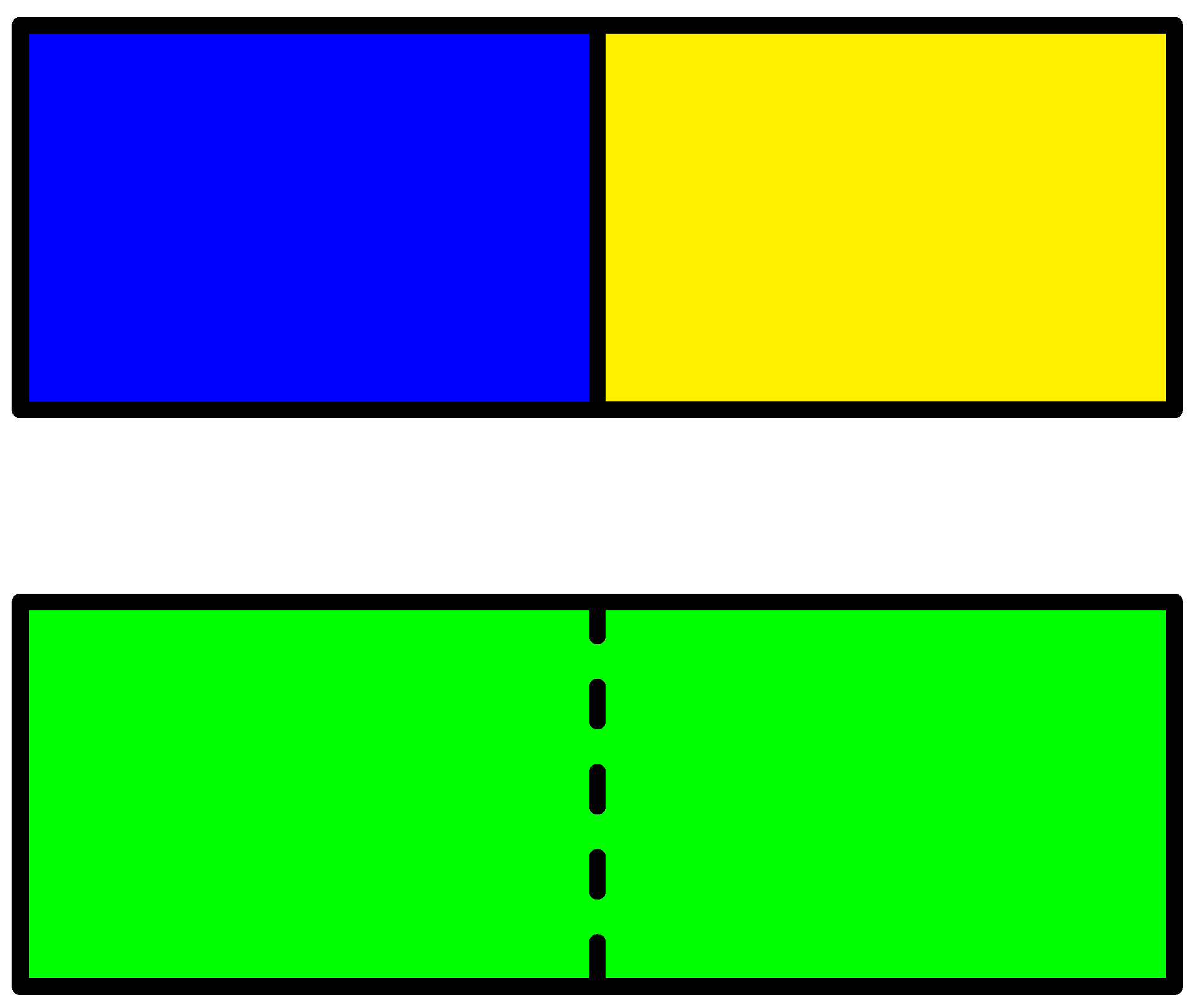
According to Equation (25) any bit of information can be converted into an amount of energy! One may ask how this is related to the mixing paradox (a special case of Gibbs’ paradox). Consider a container divided by a wall with a blue and a yellow gas on each side of the wall as illustrated in Figure 4. The question is how much energy can be extracted by mixing the blue and the yellow gas?
We loose one bit of information about each molecule by mixing the blue and the green gas, but if the color is the only difference no energy can be extracted. This seems to be in conflict with Equation (25), but in this case different states cannot be converted into each other by reversible processes. For instance one cannot convert the blue gas into the yellow gas. To get around this problem one can restrict the set of preparations and one can restrict the set of measurements. For instance one may simply ignore measurements of the color of the gas. What should be taken into account and what should be ignored, can only be answered by an experienced physicist. Formally this solves the mixing paradox, but from a practical point of view nothing has been solved. If for instance the molecules in one of the gases are much larger than the molecules in the other gas then a semi-permeable membrane can be used to create an osmotic pressure that can be used to extract some energy. It is still an open question as to which differences in properties of the two gases that can be used to extract energy.
6.4. Monotone Regret for Portfolios
We know that in general a local regret function on a state space with at least three orthogonal states is proportional to information divergence. In portfolio theory we get the stronger result that monotonicity implies that we are in the situation of gambling introduced by Kelly [35].
Theorem 7.
Assume that none of the assets are dominated by a portfolio of other assets. If the regret function given by (13) is monotone then the regret function equals information divergence and the measures P and Q are supported by k distinct price relative vectors of the form , until
Proof.
If there are more than three price relative vectors then a monotone regret function is always proportional to information divergence which is a strict regret function. Therefore we may assume that there are only two price relative vectors. Assume that the regret function is not strict. Then the function G defined by (12) is not strictly convex. Assume that so that G is affine between P and Q. Let be a contraction around one of the end points of intersection between the state space and the line through P and Q. Then monotonicity implies that so that G is affine on the line between and . This holds for contractions around any point. Therefore G is affine on the whole state space which implies that there is a single portfolio that dominates all assets. Such a portfolio must be supported on a single asset. Therefore monotonicity implies that if two assets are not dominated then the regret function is strict and according to Theorem 1 we have already proved that a strict regret function in portfolio theory is proportional to information divergence. ☐
Example 8.
If the regret function divergence is monotone and one of the assets is the safe asset then there exists a portfolio such that for all Equivalently which is possible if and only if One says that the gamble is fair if . If the gamble is super-fair, i.e., , then the portfolio gives a price relative equal to independently of what happens, which is a Dutch book.
Corollary 3.
In portfolio theory the regret function given by (13) is monotone if and only if it is strict.
Proof.
We use that in portfolio theory the regret function is monotone if and only it is proportional to information. ☐
7. Concluding Remarks
Convexity of a Bregman divergence is an important property that was first studied systematically in [56] and extended from probability distributions to matrices in [57]. In [58] it was proved that if f is a function such that the Bregman divergence based on is monotone on any (simple) C*-algebra then the Bregman divergence is jointly convex. As we have seen monotonicity implies that the Bregman divergence must be proportional to inform divergence, which is jointly convex in both arguments. We also see that in general joint convexity is not a sufficient condition for monotonicity, but in the case where the state space has only two orthogonal states it is not known if joint convexity of a Bregman divergence is sufficient to conclude that the Bregman divergence is monotone.
One should note that the type of optimization presented in this paper is closely related to a game theoretic model developed by F. Topsøe [59,60]. In his game theoretic model he needed what he called the perfect match principle. Using the terminology presented in this paper the perfect match principle states that the regret function is a strict Bregman divergence. As we have seen the perfect match principle is only fulfilled in portfolio theory if all the assets are gambling assets. Therefore, the theory of F. Topsøe can only be used to describe gambling while our optimization model can describe general portfolio theory and our sufficient conditions can explain exactly when our general model equals gambling. The formalism that has been developed in this paper is also closely related to constructor theory [61], but a discussion will be postponed to another article.
The original paper of Kullback and Leibler [1] was called “On Information and Sufficiency”. In the present paper, we have made the relation between information divergence and the notion of sufficiency more explicit. The results presented in this paper are closely related to the result that a divergence that is both an f-divergence and a Bregman divergence is proportional to information divergence (see [44] or [62] and references therein). All f-divergences satisfy a sufficiency condition, which is the reason why this class of divergences has played such a prominent role in the study of the relation between information theory and statistics. One major question has been to find reasons for choosing between the different f-divergences. For instance f-divergences of power type (often called Tsallis divergences or Cressie-Read divergences) are popular [5], but there are surprisingly few papers that can point at a single value of the power that is optimal for a certain problem except if this value is 1. In this paper we have started with Bregman divergences because each optimization problem comes with a specific Bregman divergence. Often it is possible to specify a Bregman divergence for an optimization problem and only in some of the cases this Bregman divergence is proportional to information divergence.
The idea of sufficiency has different relevance in different applications, but in all cases information divergence prove to be the quantity that convert the general notion of sufficiency into a number. In information theory information divergence appear as a consequence of Kraft’s inequality. For code length functions of integer length we get functions that are piecewise linear. Only if we are interested in extend-able sequences we get a regret function that satisfies a data processing inequality. In this sense information theory is a theory of extend-able sequences. For scoring functions in statistics the notion of locality is important. These applications do not refer to sequences. Similarly the notion of sufficiency that plays a major role in statistics, does not refer to sequences. Both sufficiency and locality imply that regret is proportional to information divergence, but these reasons are different from the reasons why information divergence is used in information theory. Our description of statistical mechanics does not go into technical details, but the main point is that the many symmetries in terms of reversible maps form a set of maps so large that our result on invariance of regret under sufficient maps applies. In this sense statistical mechanics and statistics both apply information divergence for reasons related to sufficiency. For portfolio theory the story is different. In most cases one has to apply the general theory of Bregman divergences because we deal with an optimization problem. The general Bregman divergences only reduce to information divergence when the assets are gambling assets.
Often one talks about applications of information theory in statistics, statistical mechanics and portfolio theory. In this paper we have argued that information theory is mainly a theory of sequences, while some problems in statistics and statistical mechanics are also relevant without reference to sequences. It would be more correct to say that convex optimization has various application such as information theory, statistics, statistical mechanics, and portfolio theory and that certain conditions related to sufficiency lead to the same type of quantities in all these applications.
Acknowledgments
The author want to thank Prasad Santhanam for inviting me to the Electrical Engineering Department, University of Hawai‘i at Mānoa, where many of the ideas presented in this paper were developed. I also want to thank Alexander Müller-Hermes, Frank Hansen, and Flemming Topsøe for stimulating discussions and correspondence. Finally, I want to thank the reviewers for their valuable comments.
Conflicts of Interest
The author declares no conflict of interest.
References
- Kullback, S.; Leibler, R. On Information and Sufficiency. Ann. Math. Stat. 1951, 22, 79–86. [Google Scholar] [CrossRef]
- Jaynes, E.T. Information Theory and Statistical Mechanics, I. Phys. Rev. 1957, 106, 620–630. [Google Scholar] [CrossRef]
- Jaynes, E.T. Information Theory and Statistical Mechanics, II. Phys. Rev. 1957, 108, 171–190. [Google Scholar] [CrossRef]
- Jaynes, E.T. Clearing up mysteries—The original goal. In Maximum Entropy and Bayesian Methods; Skilling, J., Ed.; Kluwer: Dordrecht, The Netherlands, 1989. [Google Scholar]
- Liese, F.; Vajda, I. Convex Statistical Distances; Teubner: Leipzig, Germany, 1987. [Google Scholar]
- Barron, A.R.; Rissanen, J.; Yu, B. The Minimum Description Length Principle in Coding and Modeling. IEEE Trans. Inf. Theory 1998, 44, 2743–2760. [Google Scholar] [CrossRef]
- Csiszár, I.; Shields, P. Information Theory and Statistics: A Tutorial; Foundations and Trends in Communications and Information Theory; Now Publishers Inc.: Delft, The Netherlands, 2004. [Google Scholar]
- Grünwald, P.D.; Dawid, A.P. Game Theory, Maximum Entropy, Minimum Discrepancy, and Robust Bayesian Decision Theory. Ann. Math. Stat. 2004, 32, 1367–1433. [Google Scholar]
- Grünwald, P. The Minimum Description Length Principle; MIT Press: Cambridge, MA, USA, 2007. [Google Scholar]
- Holevo, A.S. Probabilistic and Statistical Aspects of Quantum Theory; North-Holland Series in Statistics and Probability; North-Holland: Amsterdam, The Netherlands, 1982; Volume 1. [Google Scholar]
- Krumm, M.; Barnum, H.; Barrett, J.; Müller, M. Thermodynamics and the structure of quantum theory. arXiv, 2016; arXiv:1608.04461. [Google Scholar]
- Barnum, H.; Müller, M.P.; Ududec, C. Higher-order interference and single-system postulates characterizing quantum theory. New J. Phys. 2014, 16, 123029. [Google Scholar] [CrossRef]
- Harremoës, P. Maximum Entropy and Sufficiency. arXiv, 2016; arXiv:1607.02259. [Google Scholar]
- Harremoës, P. Quantum information on Spectral Sets. arXiv, 2017; arXiv:1701.06688. [Google Scholar]
- Barnum, H.; Lee, C.M.; Scandolo, C.M.; Selby, J.H. Ruling out higher-order interference from purity principles. arXiv, 2017; arXiv:1704.05106. [Google Scholar]
- Servage, L.J. The Theory of Statistical Decision. J. Am. Stat. Assoc. 1951, 46, 55–67. [Google Scholar]
- Bell, D.E. Regret in decision making under uncertainty. Oper. Res. 1982, 30, 961–981. [Google Scholar] [CrossRef]
- Fishburn, P.C. The Foundations of Expected Utility; Springer: Berlin/Heidelberg, Germany, 1982. [Google Scholar]
- Loomes, G.; Sugden, R. Regret theory: An alternative theory of rational choice under uncertainty. Econ. J. 1982, 92, 805–824. [Google Scholar] [CrossRef]
- Bikhchandani, S.; Segal, U. Transitive regret. Theor. Econ. 2011, 6, 95–108. [Google Scholar] [CrossRef]
- Kiwiel, K.C. Proximal Minimization Methods with Generalized Bregman Functions. SIAM J. Control Optim. 1997, 35, 1142–1168. [Google Scholar] [CrossRef]
- Kiwiel, K.C. Free-steering Relaxation Methods for Problems with Strictly Convex Costs and Linear Constraints. Math. Oper. Res. 1997, 22, 326–349. [Google Scholar] [CrossRef]
- Rockafellar, R.T. Convex Analysis; Princeton University Press: Princeton, NJ, USA, 1970. [Google Scholar]
- Hendrickson, A.D.; Buehler, R.J. Proper scores for probability forecasters. Ann. Math. Stat. 1971, 42, 1916–1921. [Google Scholar] [CrossRef]
- Rao, C.R.; Nayak, T.K. Cross Entropy, Dissimilarity Measures, and Characterizations of Quadratic Entropy. IEEE Trans. Inf. Theory 1985, 31, 589–593. [Google Scholar] [CrossRef]
- Banerjee, A.; Merugu, S.; Dhillon, I.S.; Ghosh, J. Clustering with Bregman Divergences. J. Mach. Learn. Res. 2005, 6, 1705–1749. [Google Scholar]
- Kraft, L.G. A Device for Quanitizing, Grouping and Coding Amplitude Modulated Pulses. Master’s Thesis, Department of Electrical Engineering, MIT University, Cambridge, MA, USA, 1949. [Google Scholar]
- Han, T.S.; Kobayashi, K. Mathematics of Information and Coding; Translations of Mathematical Monographs; American Mathematical Society: Providence, RI, USA, 2002; Volume 203. [Google Scholar]
- De Finetti, B. Theory of Probability; Wiley: Hoboken, NJ, USA, 1974. [Google Scholar]
- McCarthy, J. Measures of the value of information. Proc. Natl. Acad. Sci. USA 1956, 42, 654–655. [Google Scholar] [CrossRef] [PubMed]
- Gneiting, T.; Raftery, A.E. Strictly Proper Scoring Rules, Prediction, and Estimation. J. Am. Stat. Assoc. 2007, 102, 359–378. [Google Scholar] [CrossRef]
- Ovcharov, E.Y. Proper Scoring Rules and Bregman Divergences. arXiv, 2015; arXiv:1502.01178. [Google Scholar]
- Gundersen, T. An Introduction to the Concept of Exergy and Energy Quality; Lecture notes; Norwegian University of Science and Technology: Trondheim, Norway, 2011. [Google Scholar]
- Harremoës, P. Time and Conditional Independence; IMFUFA-Tekst; IMFUFA Roskilde University: Roskilde, Denmark, 1993; Volume 255. [Google Scholar]
- Kelly, J.L. A New Interpretation of Information Rate. Bell Syst. Tech. J. 1956, 35, 917–926. [Google Scholar] [CrossRef]
- Cover, T.M.; Thomas, J.A. Elements of Information Theory; Wiley: Hoboken, NJ, USA, 1991. [Google Scholar]
- Cover, T.M. Universal portfolios. Math. Finance 1991, 1, 1–29. [Google Scholar] [CrossRef]
- Uhlmann, A. On the Shannon Entropy and Related Functionals on Convex Sets. Rep. Math. Phys. 1970, 1, 147–159. [Google Scholar] [CrossRef]
- Müller-Hermes, A.; Reeb, D. Monotonicity of the Quantum Relative Entropy under Positive Maps. Annales Henri Poincaré 2017, 18, 1777–1788. [Google Scholar] [CrossRef]
- Christandl, M.; Müller-Hermes, A. Relative Entropy Bounds on Quantum, Private and Repeater Capacities. arXiv, 2016; arXiv:1604.03448. [Google Scholar]
- Petz, D. Monotonicity of Quantum Relative Entropy Revisited. Rev. Math. Phys. 2003, 15, 79–91. [Google Scholar] [CrossRef]
- Petz, D. Sufficiency of Channels over von Neumann algebras. Q. J. Math. Oxf. 1988, 39, 97–108. [Google Scholar] [CrossRef]
- Jenčová, A.; Petz, D. Sufficiency in quantum statistical inference. Commun. Math. Phys. 2006, 263, 259–276. [Google Scholar] [CrossRef]
- Harremoës, P.; Tishby, N. The Information Bottleneck Revisited or How to Choose a Good Distortion Measure. In Proceedings of the IEEE International Symposium on Information Theory, Nice, France, 24–29 June 2007; pp. 566–571. [Google Scholar]
- Jiao, J.; Courtade, T.A.; No, A.; Venkat, K.; Weissman, T. Information Measures: The Curious Case of the Binary Alphabet. IEEE Trans. Inf. Theory 2014, 60, 7616–7626. [Google Scholar] [CrossRef]
- Jenčová, A. Preservation of a quantum Rényi relative entropy implies existence of a recovery map. J. Phys. A Math. Theor. 2017, 50, 085303. [Google Scholar] [CrossRef]
- Tishby, N.; Pereira, F.; Bialek, W. The information bottleneck method. In Proceedings of the 37th Annual Allerton Conference on Communication, Control and Computing, Urbana, Illinois, USA, 22–24 September 1999; pp. 368–377. [Google Scholar]
- No, A.; Weissman, T. Universality of logarithmic loss in lossy compression. In Proceedings of the 2015 IEEE International Symposium on Information Theory (ISIT), Hongkong, China, 14–19 June 2015; pp. 2166–2170. [Google Scholar]
- Dawid, A.P.; Lauritzen, S.; Perry, M. Proper local scoring rules on discrete sample spaces. Ann. Stat. 2012, 40, 593–603. [Google Scholar] [CrossRef]
- Bernardo, J.M. Expected Information as Expected Utility. Ann. Stat. 1978, 7, 686–690. [Google Scholar] [CrossRef]
- Csiszár, I. Why least squares and maximum entropy? An axiomatic approach to inference for linear inverse problems. Ann. Stat. 1991, 19, 2032–2066. [Google Scholar] [CrossRef]
- Bartlett, P.; Grünwald, P.; Harremoës, P.; Hedayati, F.; Kotlowski, W. Horizon-Independent Optimal Prediction with Log-Loss in Exponential Families. In Proceedings of the Conference on Learning Theory (COLT 2013), Princeton, NJ, USA, 12–14 June 2013; p. 23. [Google Scholar]
- Lieb, E.; Yngvason, J. A Guide to Entropy and the Second Law of Thermodynamics. Not. AMS 1998, 45, 571–581. [Google Scholar]
- Lieb, E.; Yngvason, J. The Mathematics of the Second Law of Thermodynamics. In Visions in Mathematics; Alon, N., Bourgain, J., Connes, A., Gromov, M., Milman, V., Eds.; Birkhäuser: Basel, Switzerland, 2010; pp. 334–358. [Google Scholar]
- Marletto, C. Constructor Theory of Thermodynamics. arXiv, 2016; arXiv:1608.02625. [Google Scholar]
- Bauschke, H.H.; Borwein, J.M. Joint and Separate Convexity of the Bregman Distance. In Inherently Parallel Algorithms in Feasibility and Optimization and Their Applications; Dan Butnariu, Y.C., Reich, S., Eds.; Elsevier: Amsterdam, The Netherlands, 2001; Volume 8, pp. 23–36. [Google Scholar]
- Hansen, F.; Zhang, Z. Characterisation of Matrix Entropies. Lett. Math. Phys. 2015, 105, 1399–1411. [Google Scholar] [CrossRef]
- Pitrik, J.; Virosztek, D. On the Joint Convexity of the Bregman Divergence of Matrices. Lett. Math. Phys. 2015, 105, 675–692. [Google Scholar] [CrossRef]
- Topsøe, F. Game theoretical optimization inspired by information theory. J. Glob. Optim. 2008, 43, 553–564. [Google Scholar] [CrossRef]
- Topsøe, F. Cognition and Inference in an Abstract Setting. In Proceedings of the Fourth Workshop on Information Theoretic Methods in Science and Engineering (WITMSE 2011), Helsinki, Finland, 7–10 August 2011; pp. 67–70. [Google Scholar]
- Deutch, D.; Marletto, C. Constructor theory of information. Proc. R. Soc. A 2014, 471, 20140540. [Google Scholar] [CrossRef] [PubMed]
- Amari, S.I. α-Divergence Is Unique, Belonging to Both f-Divergence and Bregman Divergence Classes. IEEE Trans. Inf. Theory 2009, 55, 4925–4931. [Google Scholar] [CrossRef]
Figure 1.
The regret equals the vertical distance between curve and tangent.
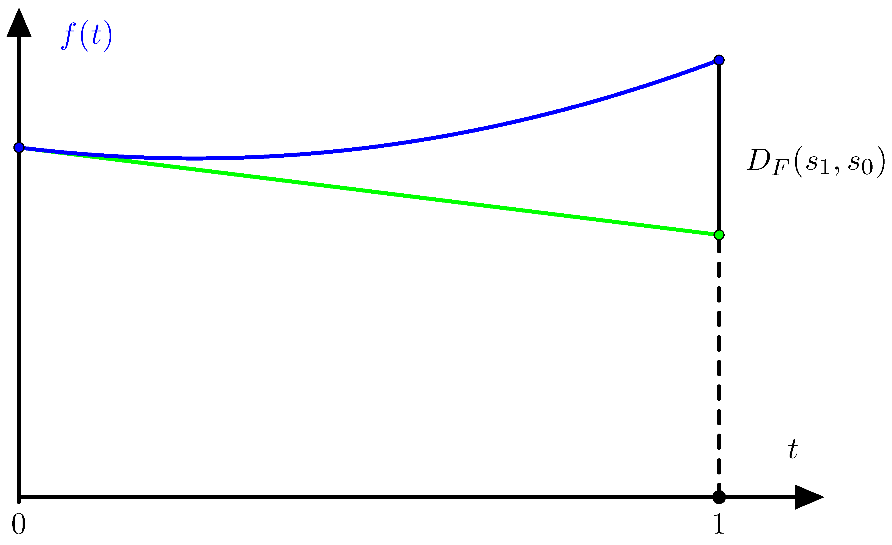
Figure 2.
The function G for the price relative vectors in Example 4.
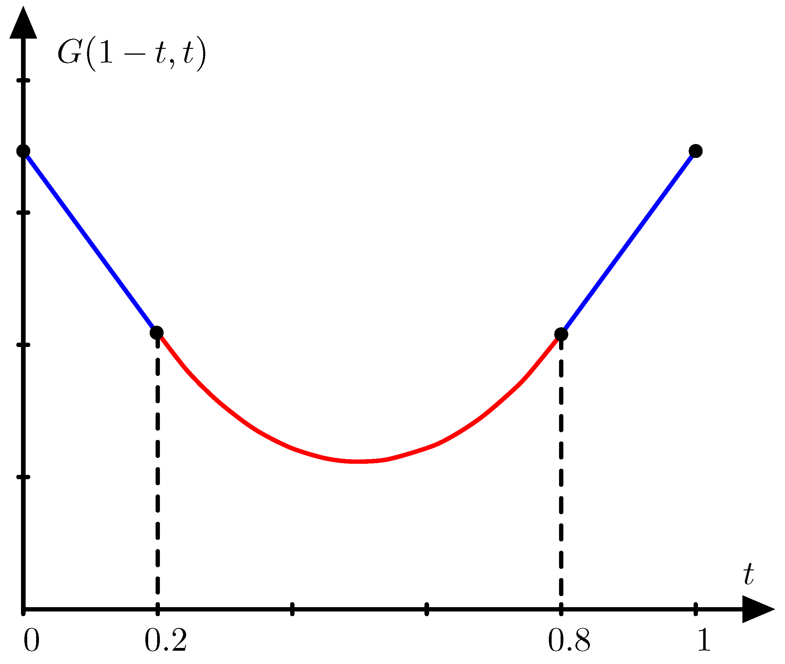
Figure 3.
Example of a dilation that increases regret.

Figure 4.
Mixing of a blue and a yellow gas.
© 2017 by the author. Licensee MDPI, Basel, Switzerland. This article is an open access article distributed under the terms and conditions of the Creative Commons Attribution (CC BY) license (http://creativecommons.org/licenses/by/4.0/).
Share and Cite
MDPI and ACS Style
Harremoës, P. Divergence and Sufficiency for Convex Optimization. Entropy 2017, 19, 206. https://doi.org/10.3390/e19050206
AMA Style
Harremoës P. Divergence and Sufficiency for Convex Optimization. Entropy. 2017; 19(5):206. https://doi.org/10.3390/e19050206
Chicago/Turabian StyleHarremoës, Peter. 2017. "Divergence and Sufficiency for Convex Optimization" Entropy 19, no. 5: 206. https://doi.org/10.3390/e19050206
Note that from the first issue of 2016, this journal uses article numbers instead of page numbers. See further details here.