
Utility, Revealed Preferences Theory, and Strategic Ambiguity in Iterated Games


Complex Systems Research Group, Faculty of Engineering and Information Technologies, The University of Sydney, Sydney NSW 2006, Australia
Entropy 2017, 19(5), 201; https://doi.org/10.3390/e19050201
Submission received: 28 February 2017
/
Revised: 10 April 2017
/
Accepted: 26 April 2017
/
Published: 29 April 2017
(This article belongs to the Special Issue Complexity, Criticality and Computation (C³))
Abstract
:Iterated games, in which the same economic interaction is repeatedly played between the same agents, are an important framework for understanding the effectiveness of strategic choices over time. To date, very little work has applied information theory to the information sets used by agents in order to decide what action to take next in such strategic situations. This article looks at the mutual information between previous game states and an agent’s next action by introducing two new classes of games: “invertible games” and “cyclical games”. By explicitly expanding out the mutual information between past states and the next action we show under what circumstances the explicit values of the utility are irrelevant for iterated games and this is then related to revealed preferences theory of classical economics. These information measures are then applied to the Traveler’s Dilemma game and the Prisoner’s Dilemma game, the Prisoner’s Dilemma being invertible, to illustrate their use. In the Prisoner’s Dilemma, a novel connection is made between the computational principles of logic gates and both the structure of games and the agents’ decision strategies. This approach is applied to the cyclical game Matching Pennies to analyse the foundations of a behavioural ambiguity between two well studied strategies: “Tit-for-Tat” and “Win-Stay, Lose-Switch”.
1. Introduction
Game theory as it was originally framed by von Neumann and Morgenstern [1] and Nash [2] is concerned with agents (decision-makers) selecting actions to take when they interact strategically with other agents. Strategic interactions in the economic sense are situations in which the reward, or utility, one agent receives is based upon the action they choose to take as well as the actions taken by other agents. In much of non-cooperative game theory [3], it is assumed that agents are maximising their personal utility in one-off encounters between agents that know nothing of past behaviours, and that they choose their actions independently of one another, i.e., they do not discuss their strategies or collaborate with one another before choosing their actions. Relaxing these assumptions has been very fruitful in understanding the fundamental principles of strategic interactions: repeated games with learning can lead to chaotic dynamics [4] and spatially structured games can lead to cooperation where cooperation would not usually occur [5] or to a lack of cooperation where cooperation would usually occur [6].
An important approach to broadening the interaction model between agents has been to include interactions over time, as opposed to a single one-off game, and this has a significant impact on the possible outcomes. Each game can be thought to have occurred at a discrete point in time, i.e., agents’ moves and utilities are said to occur at time t, and then consider what choices the agents then make at time based on the moves and utilities at time t, , etc. These are called iterated games and they have been extensively studied by Axelrod [7], Nowak [8] and many others. In order to explore this approach, Axelrod ran a tournament in which contestants submitted algorithms that would compete against each other in playing a game, the Prisoner’s Dilemma (see below for details), in which the algorithm that accumulated the highest utility would be the winner. The winning algorithm, submitted by Anatol Rapport [9], played a very simple strategy called Tit-for-Tat in which the algorithm initially cooperates with its opponent and thereafter chooses the strategy its opponent had used in the prior round. These and subsequent results led to a series of fundamental insights into the complexity of strategic interactions in dynamic games [10,11,12,13].
The real-valued utilities in game theory play an important role in many artificial intelligent systems such as those that use reinforcement learning, but in economic theory, it is the agent’s behaviour that reveals an agent’s subjective preferences. In the introduction to Rational Decisions ([14], p. 8), Ken Binmore discusses “revealed preference theory”, the current economic orthodoxy on subjective utility. The theory states that if a decision-maker consistently acts to select one option over another, then their subjective preferences are revealed by their behaviour and their acts can be interpreted as if they are maximising a real valued utility function (see Savage’s The Foundations of Statistics [15] for subjective preferences). The alternative point of view, that decision-makers act consistently because they have an internal real-valued utility function that allows them to order their choices, is called the causal utility fallacy (see pp. 19–22 of Rational Decisions [14]). For a review of earlier work and an historical discussion of the central role it has played in the foundations of economic theory see Chapter 1 in [16].
Revealed preferences freed economists from needing to consider the psychological or procedural aspects of choice to instead focus on agent behaviour. As a consequence, it should be possible to infer an agent’s preferences from their behaviours alone, independently of the values of the utilities. In the non-cooperative game theory introduced in Section 2, we introduce the utility bi-matrices and prove their redundancy for iterated games in Section 3 using elementary results based on information theory. Corollary 1 specifically shows that the utility can be replaced by the previous acts of both agents in determining the next choice for any strategy in a two person iterated game. This appears to be the first time that this fundamental principle has been derived using information theory. The Traveller’s Dilemma and the Prisoner’s Dilemma illustrate this point in Section 4.
Regardless of the revealed preferences theory, significant work has focused on the neuro-computational processes that result in particular strategic behaviours [16,17,18] and so the relationship between observed behaviour and the computations that underlie that behaviour is of practical interest. However, it has been noted [19] that there are certain games for which an agent’s choices are consistent with multiple different cognitive processes, and we show in Section 4 that these can be of distinctly different levels of complexity. This does not refute revealed preference theory; it only shows that the theory is limited insofar as it cannot distinguish between different internal processes, see [20], particularly footnote 8 and Conclusions, for a neuro-economic view of the internal cognitive states that are considered irrelevant to revealed preferences. In order to analyse the coupled interaction between games and strategies, they both need to be expressed in the same formal language, and this is done by describing games and strategies in terms of logic gates via truth tables and the computational processes that result in this ambiguity are described. In Section 4, we apply two well studied strategies (Tit-for-Tat and Win-Stay, Lose-Shift) to the Matching Pennies game and show that identical behaviours would require qualitatively different artificial neural networks to minimally implement. These two strategies, applied to iterated games as we do in this article, have been pivotal to the modern understanding of strategic evolution in game theory (see [11] and Chapters 4–5 of [8]). This illustrates a key limitation in revealed preferences theory: under certain conditions, it is not possible to know a market’s composition of “herders” and “fundamentalists” by observing behaviour alone, an important factor in financial market collapse [21,22]. These points are discussed at the end of Section 5.
2. Non-Cooperative Game Theory
A normal form, non-cooperative game is composed of agents who are each able to select an act (often called a “pure strategy” in game theory) () where the joint acts of all agents collectively determines the utility for each agent i, . An act is said to be preferable to an act via the utility function if we have: . We use to denote agent i’s utility function, taking joint action as an argument, and as the utility value (a real number) for agent i in the n-th round of an iterated game (see below), if there is any uncertainty as to which agent’s utility value we are referring to, we use . We will represent the actions available to the agents and their subsequent utility values using the conventional bi-matrix notation—for example, the Prisoner’s Dilemma [23] is given by the following payoff bi-matrix in Table 1 (by convention, i indexes the agent being considered, indexes the other agent):
In this game, there are two agents (prisoners held in two different jail cells) who have been arrested for a crime and they are being questioned (independently) by the police regarding the crime. Each agent chooses from the same set of possible acts: cooperate with their fellow detainee and remain silent about the crime or defect and tell the police about the crime and implicate their fellow detainee. If they both cooperate with each other, they each get one year in jail, if they both defect, they each get three years in jail, if one defects and one cooperates the defector gets no jail time (zero years) while the cooperator gets five years in jail. We also define a game’s state space for agent i, a specific set of acts and utilities (variables) for agent i—for example, co-op, defect, five years} is a specific state space of variables when i cooperates and defects. The variables in are deterministically related to one another via the bi-matrix of the game being played. The following definitions form the two sub-classes of games that we will use in the following section:
Definition 1.
Invertible Games: An invertible game for agent i is a game for which each of i’s real-valued utilities uniquely defines the joint actions of all agents. A game is invertible if it is invertible for all agents.
For example, the Prisoner’s Dilemma and Stag Hunt games are invertible but the Matching Pennies and Rock–Paper–Scissors games are not. Matching Pennies and Prisoner’s Dilemma are discussed in detail below, and see, for example, [24] for Rock, Paper, Scissors and [25] for Stag Hunt.
Definition 2.
Cyclical Games: Given the cardinality of variables in agent i’s state space , a cyclical game for agent i is a game for which knowing any combination of variables of is both necessary and sufficient to derive the remaining variable. A game is cyclical if it is cyclical for all agents.
The Prisoner’s Dilemma is not cyclical, Matching Pennies and Rock-Paper-Scissors are cyclical but the Traveler’s Dilemma (see Section 4: Example Games) is neither invertible nor cyclical.
3. Information Theory
Information theory measures the degree of stochastic variability and dependency in a system based on the probability distributions that describe the relationships between the elements of the system. For a discrete stochastic variable the (Shannon) Entropy is:
measured in bits as assumed throughout, and this is maximised if x is uniformly distributed over all and zero if for any i. We will write or if there is no confusion. There are many possible extensions to the notion of Entropy, in this work, we will make use of the Mutual Information and the conditional Mutual Information, respectively defined as [26]:
If, in Equation (1), there is a (deterministic, linear or nonlinear) mapping then and . Similarly, for Equation (2), if there is a (deterministic, linear or nonlinear) mapping such that , then the summation reduces to a weighted sum over and and so bits.
A useful special case of the conditional mutual information is the Transfer Entropy (TE) [27]. For a system with two stochastic variables X and Y that have discrete realisations and at time points then the TE of the joint time series: is the mutual information between one variable’s current state and the second variable’s next state conditional on the second variable’s current state:
This is interpreted as the degree to which the previous state of Y is informative about the next state of X excluding the past information X carries about its next state. This is one of many different specifications of TE, generalisations based on history length appears in Schreiber’s original article [27], and further considerations of delays [28] as well as averaging the TE over whole systems of stochastic variables [29] have also been developed (for a recent review, see [30]).
In iterated games, we wish to know how much information passes from each variable in agent i’s state space at time n to their next act and what simplifications can be made. It is assumed that each agent i has a strategy that maps previous system states to actions at time and, in general, this may depend on system states of an arbitrary length of time into the past:
where is assumed to be the totality of an agent’s information set used to make a decision. For example, one of the simplest 1-step strategies is the Tit-for-Tat (TfT) strategy, whereby agent i simply copies the previous act of the other agent [8,9]:
It is possible for to take no arguments in which case the agent chooses from a distribution over their next act that is independent of any information set. This is the case for the Matching Pennies game considered below: two agents simultaneously toss one coin each and the outcome, either matched coins or mismatched coins, decides the payoff to either agent and so for this “0-step strategy” each action is independent of all past states of the game for both agents. Given a maximum history length of l, we will say that a strategy is an l-step Markovian strategy and an l-step Markovian game is a sequence of the same game played repeatedly for which each agent has an l-step Markovian strategy.
Information Chain Rule and Iterated Games
We are interested in constructing probability distributions over the variables in for iterated games. As n indexes time, for large a probability of an event is the frequency of occurrence of the event (an element in ) divided by n. Other probabilities, such as conditional or joint probabilities, are natural extensions of this approach. For the moment, we make no assumptions about the relationship between elements of and except that they are not statistically independent of each other. Given a 2-agent, 1-step Markovian game with states , from the chain rule for information ([26], Theorem 2.5.2), we have the following six identities for the total information between the previous game state and agent i’s subsequent act :
We will say that measures the amount of information shares with . These expressions for the shared information between game states and next actions can be simplified in useful ways as follows:
Theorem 1.
For any normal form, non-cooperative 1-step Markovian game (not necessarily cyclical or invertible): for the joint act .
Proof.
From the definition of a non-cooperative game, the utility value is determined by the joint strategies so the log term in Equation (2) can be written: . In this case, both conditional probabilities in the log term will be either 0 or 1 and note the discussion following Equation (2). ☐
Remark 1.
From Theorem 1, the first terms in Equations (6e) and (6f) are zero. While the joint actions of the agents unambiguously identifies a utility value, in general the utility value does not unambiguously identify a joint action. See the Traveler’s Dilemma example below.
Corollary 1.
For a 2-agent, 1-step Markovian game, the total information from agent i’s previous state space to i’s next act is encoded in the sum of agent i’s Transfer Entropy from agent ’s previous act to agent i’s current act and agent i’s “active memory” [31] of their own past acts:
Proof.
By Theorem 1 and Equation (6e). ☐
Theorem 2.
For a 2-agent, invertible 1-step Markovian game .
Proof.
This follows the same approach as Theorem 1 where knowing the joint act implies knowing any single agent’s act and from the definition of an invertible game for which is the necessary deterministic map. ☐
Remark 2.
From Theorem 2, the first terms in Equations (6a)–(6f) are zero for invertible 1-step Markovian games.
Corollary 2.
For an invertible 1-step Markovian game, the total information from agent i’s previous state space to agent i’s next act is encoded in agent i’s active memory between the previous utility and their subsequent act:
Proof.
By Theorem 2 for Equation (6c): and so: . ☐
Theorem 3.
For a cyclical 1-step Markovian game, .
Proof.
This follows the same approach as Theorem 1 and note that, for a three element in a cyclical game, there is a and distinct , for which there is a deterministic relationship between any pairing of a or b with c and, consequently, the conditional mutual information in Theorem 3 is zero. ☐
Remark 3.
From Theorem 3, the first term in Equations (6a)–(6f) are zero for cyclical 1-step Markovian games.
Corollary 3.
For a cyclical or an invertible 2-agent, 1-step Markovian game:
Proof.
This comes from Theorems 2 and 3 and comparing Equation (6a) with (6f), Equation (6b) with (6e) and Equation (6c) with (6d). ☐
Remark 4.
Equality (8) is notable, and it states that the transfer entropy from the utility of agent i to their next act is the same as the transfer entropy from agent ’s act to agent i’s next act.
4. Example Games
In this section, we consider in some detail three games belonging to three distinct classes. The first example, the Traveler’s Dilemma, belongs to the class of games that are neither invertible nor cyclical. The second example, the Prisoner’s Dilemma, is an invertible game and the final example, the Matching Pennies game, is a cyclical game. The Traveler’s Dilemma and the Prisoner’s Dilemma illustrate the information theoretical aspects of iterated games and the Matching Pennies game illustrates the computational properties of cyclical games.
4.1. The Traveler’s Dilemma
The story describing the Traveler’s Dilemma (TD) game is often told in the following form [32]:
“Lucy and Pete, returning from a remote Pacific island, find that the airline has damaged the identical antiques that each had purchased. An airline manager says that he is happy to compensate them but is handicapped by being clueless about the value of these strange objects. Simply asking the travelers for the price is hopeless, he figures, for they will inflate it.Instead, he devises a more complicated scheme. He asks each of them to write down the price of the antique as any dollar integer between $2 and $100 without conferring together. If both write the same number, he will take that to be the true price, and he will pay each of them that amount. However, if they write different numbers, he will assume that the lower one is the actual price and that the person writing the higher number is cheating. In that case, he will pay both of them the lower number along with a bonus and a penalty–the person who wrote the lower number will get $2 more as a reward for honesty and the one who wrote the higher number will get $2 less as a punishment. For instance, if Lucy writes $46 and Pete writes $100, Lucy will get $48 and Pete will get $44.”
The utility function for the TD game can be defined using the Heaviside step function :
and agent i’s action is the cost i claims for the vase and agent ’s action is the cost claims for the vase, the utility for agent i is [33]:
This game is not invertible because, in the case where the two agents disagree with each other, the agent i who offers the lowest value has a utility of whereas the other agent has a utility of , i.e., agent ’s utility is independent of the precise value offered; therefore, the agent utility is invertible for agent i but not for agent , so the game is not invertible. For iterated TD games, the simplest calculation of the information shared between the previous state and the next action is: .
4.2. Prisoner’s Dilemma
The Prisoner’s Dilemma is one of the most well studied economic games. It was originally an experimental test in a repeated game format by researchers at the RAND Corporation (Santa Monica, CA, USA) who were skeptical of Nash’s notion of equilibrium on the basis that no real players would play in the fashion Nash had proposed [23]. Here, we use it to illustrate that utility can be used exclusively to learn strategies just as behaviour can be used to exclusively learn better strategies. In the second part of this example, we use Nowak’s approach [8] to understand the relationship between information sets, game structure and strategies. The logic gate approach allows us to express games and strategies in the same language, allowing a direct comparison of game structure and strategies. The Prisoner’s Dilemma (PD) was introduced earlier, see the payoff matrix in Table 1.
Because it is invertible for both agents (from the uniqueness of each of the four utilities for each agent), the total information from the previous time step to the next act for either agent is encoded in the Mutual Information between the previous utility and the next act: . For a 1-step Markovian strategy, no other past information is needed to select the next act. In this sense, the utility acts as a reward that an agent can use to distinguish between the actions of other players, and the entire joint action space of the game’s previous state can be reconstructed by agent i using only the utility value.
To explore this further, we follow Nowak ([8], pp. 78–89) in defining two deterministic strategies in the iterated version of the PD game in terms of previous game states and subsequent acts. In the iterated PD, there are four possible joint acts at time n: , , and . The action of the agent we are referring to, usually indexed as i, has their act in capital letters i.e., C and D for cooperate and defect, whereas the other agent has lower case acts c or d. A vector of these joint acts is mapped to a vector of acts at time in the following way: where . In the Tit-for-Tat strategy (TfT): in which agent i copies the other agent’s previous act, and in the Win-Stay, Lose-Switch strategy (WSLS): in which agent i repeats their act if they receive a high payoff (a `win’ of either 1 or 0 years) but changes their act if they receive a low payoff (a `loss’ of three or five years). This interpretation of the WSLS strategy is not an accurate representation of the strategy though: WSLS monitors the success (measured by utility) of the previous act and adjusts the next act accordingly i.e., WSLS uses the information set to select , not as is implied by the representation . This distinction is not important for Nowak’s analysis of PD [8] (p. 88), but it is important in the analysis below.
It can be seen that these two strategies have the same amount of shared information between their previous game states and their next acts: TfT ≃ WSLS. Note that we consider agent ’s actions to be uniformly distributed across their possible acts, whereas agent i follows one of the deterministic strategies described next. We use ≃ and ≡ to distinguish between having the same quantity of information (≃) and having the same observed behaviour (≡). For TfT, the shared information between and is: bit. The two expansions of that contain this mutual information term are Equations (6a) and (6f), so the first two terms in these two equations must be zero for PD. The first term is zero by Theorem 2, and we observe that in TfT explicitly determines , so the second conditional entropy terms in which conditions must also be zero. For WSLS, we measure in terms of and then show that this is equivalent to the TfT result. By Theorem 2 for invertible games, the first term in any expansion of is zero, and the equations that then only have in their expression are Equations (6b) and (6c). These equations measure the shared information between the information set of WSLS and the agent’s next act, i.e., . Equation (6c) is then: and by Corollary 2 —by definition, Equation (6c) ≃ Equation (6a) and, therefore, . However, TfT is not behaviourally equivalent to WSLS for the PD: WSLS TfT as can be seen by direct comparison of the strategies described above.
We now consider the relationship between WSLS and TfT for the PD game by making the following substitutions: , , a “win” , and a “loss” . Replacing the utilities with a win–loss binary variable is justified as WSLS (the only strategy that uses the utilities) only considers wins and losses, not the numerical values of the utilities. It can then be seen that this modified version of the Prisoner’s Dilemma is equivalent to a NOT logic gate for agent i that inverts the action of agent (see Table 2):
The first three columns in Table 2 are the actions of the two agents in round n of an iterated game and the outcome of the game based on these actions, i.e., each row is an instance of the 3-element set . The next two columns of Table 2 are the actions of agent i in round for WSLS and TfT. The diagram shows the relationship between the elements in when the game is interpreted as a logic gate relating inputs (agent actions) and outputs (wins and losses). In this case, the 4 × 3 matrix made up of the four rows of possible combinations of is the “truth table” of the PD game. Note that, while both agents always have an incentive to defect irrespective of what the other agent does (defection is said to strictly dominate cooperation, see ([34], p. 10)), it is only agent ’s action that decides whether or not agent i will win or lose. Whether this is a large or a small win or loss is controlled by agent i though, and this aspect was lost when the utility was made into a binary win–loss outcome in modifying the PD game in the table. Figure 1 represents these relationships for TfT being played in an iterated PD game.
Next, we show that WSLS is a nonlinear function of its two inputs while TfT is a linear function of its inputs. To see this, note that TfT ≃ WSLS and TfT is linearly (anti-)correlated with win–loss; however, there is zero pairwise linear correlation between WSLS actions and either or . Consequently, because mutual information measures both linear and nonlinear relationships between variables, all of the shared information between and is either linear for TfT or nonlinear for WSLS.
A truth table can also be constructed from the information set of WSLS (columns 1 and 3 in Table 2) and the WSLS action in the next round (column 4 in Table 2) and the truth table is that of an XNOR (exclusive-nor) logic gate in which matching inputs (00 or 11) are mapped to 0 and mismatched inputs (10 or 01) are mapped to 1. Encoding the utilities of the PD as win–loss and representing it as a NOT gate makes clear that learning the relationships between the variables of for the PD game (as encoded in the first three columns of the table above) is a linearly separable task; if agent i wants to learn the PD, it only needs to divide the state space of agent ’s actions up into wins and losses for agent i, a problem that can be solved by single layer perceptrons [35]. However, learning the WSLS strategy, equivalent to learning an XNOR operation, is not a linearly separable task and requires a multi-layer perceptron [36]. Figure 2 represents these relationships for WSLS being played in an iterated PD game.
In the modified PD, the utility values were converted to binary variables, and this works because TfT does not have the utility value in its information set and WSLS has the utility value in its information set but only considers the outcome as a binary win–loss variable. In the next example, these substitutions are unnecessary. We take a similar approach to establish that the Matching Pennies game is not a linearly separable problem and that WSLS is both informationally and behaviourally identical to TfT for one agent but not the other.
4.3. Matching Pennies
The Matching Pennies (MP) game is an important example used in laboratory studies [19] of economic choice, learning and strategy. In the MP game, two agents have one coin each and each coin has two states, either Heads (H) or Tails (T). When the agents compare coins one agent wins if the two coins match and the other agent wins if they do not match. In the usual description of the game, the two agents toss their coins before comparing them; this randomising of the coin states can be interpreted as one step of an iterated game using a 0-step Markovian strategy. In what follows, though, we use the name “Matching Pennies” to describe the iterated game where the WSLS and TfT are deterministic strategies that use the action-utility bi-matrix given by (see Table 3):
In the same fashion as for the PD game above, we can map agents’ acts to numerical values: , , and a win = 1, a loss = 0 (unlike the PD game, we do not need to simplify the utility values and so the game is not modified as the PD was). Then, the MP game can be interpreted as XNOR (exclusive-nor) and XOR (exclusive-or) gates in the following two tables (see Table 4 and Table 5) for the two agents:
As for the PD game, the first three columns of each row in Table 4 and Table 5 represent an instance of (Table 4) and (Table 5), and the four possible permutations of the variables of and forms a 4 × 3 table that can be interpreted as the truth table of a logic gate. However, unlike in the PD game, both agents now have an input into each other’s logic gate (see Figure 3 and Figure 4 for schematic representations for agent i). Just as in the PD, for MP, the WSLS strategy is not linearly correlated with any element of its information set and TfT is linearly correlated with its information set; recall the WSLS information set for agent i’s act is and the TfT information set is . However, unlike the PD, now WSLS is perfectly (linearly) correlated with TfT for agent i and perfectly anti-correlated for agent .
It can also be seen that knowing any two variables in is sufficient to derive the third variable. This is a property of the XOR (⊕) and XNOR () logic operations; given the three variables related by the XNOR operator, then: , , and , and we will refer to this as the cyclical property of cyclical games. We can now prove the following relationship:
Theorem 4.
TfT ≡ WSLS for agent i: for the Matching Pennies iterated game, the Tit-for-Tat strategy is behaviourally indistinguishable from the Win-Stay-Lose-Shift strategy for agent i.
Proof.
By the cyclical property for Matching Pennies, if: , then . The WSLS strategy takes these same inputs but outputs : . Because and are equivalent to XNOR logic gates, for the same input, they produce the same output: and therefore . By definition, the TfT strategy is and so TfT ≡ WSLS. ☐
Remark 5.
TfT is a prototypical herd-like strategy: it simply follows the behaviour of another agent. In contrast, WSLS is a prototypical fundamental strategy: it uses past actions and their payoffs to decide whether to stay with the current strategy or change. The fact that they are indistinguishable from each other is not guaranteed; for the Prisoner’s Dilemma, TfT is behaviourally distinguishable from WSLS, and the indistinguishability in the Matching Pennies game comes from identifying the MP game and the WSLS strategy with the same (XNOR) logic gate and the cyclical property of .
Before the next result, we introduce a variation on the WSLS strategy, called “Win-Switch-Lose-Stay”: WSLS in which an agent changes strategy if they win but will stay with a losing strategy.
Corollary 4.
TfT ≡ WSLS for agent .
Proof.
The XOR logic gate for agent shows the WSLS strategy is anti-correlated with the TfT strategy; this is the opposite behaviour of the XNOR logic gate for agent i, so flipping the behaviours of WSLS: and results in the strategy WSLS that is behaviourally the same as TfT. In Nowak’s notation in the Matching Pennies game for agent (who wins if pennies are mismatched), this results in an inverted WSLS: , which is equivalent to . ☐
The TfT strategy for the MP game is a linearly separable learning task, given a single layer perceptron is sufficient to map to the correct output [35]. The WSLS strategy for the MP game is not a linearly separable task because it is equivalent to an XNOR gate [36]: given , a multi-layer perceptron is necessary to map and to . This difference in the complexity of the computational task and the indistinguishable character of the subsequent behaviour of the agents suggests that understanding cognitive decision-making processes is not easily untangled by observing behaviour.
5. Discussion
This article uses Transfer Entropy in the analysis of iterated games while also contributing theoretical concepts to the analysis of the computational foundations of games and strategies (work on Matching Pennies can be found in [37] using a different measure of `information flow’). In some respects, the analysis of games discussed here is very similar to the Elementary Cellular Automata (ECAs) work of Lizier and colleagues [38,39]. In ECAs, the number of agents is much larger than the two agent games considered here, and they form a potentially infinite spatial array of locally connected agents that switch states based on their own states and the states of their neighbours. ECAs are simpler than the agents considered in this article as they do not have a utility function associated with their collective behaviour, an added complexity that has been shown here to be either informative or redundant depending on the game and the strategy being played. The possibility that utility values are redundant is important in reward based learning and it is a poorly studied area. This can be seen in economic theory in which “revealed preference theory” plays a significant role in understanding the connection between behaviour and reward. The analogy between iterated games and elementary cellular automata has been studied earlier by in [40,41]. An important property of these ECAs is that they are massively parallel computational systems and some, such as Wolfram’s rule 110, are capable of universal computation [42]. This is very different to conventional approaches to understanding economic foundations. The focus in economics is often on finding equilibrium solutions [43], whereas, in ECAs, the emphasis is on the dynamical properties of the system. From this perspective, ECAs have been studied as dynamical systems made up of parallel logic gates (see [44], p. 81) while logic gates have recently played an important role in information theory [45] and the computational biology of neural networks [46].
The classification of games and strategies as logic gates also has analogies in ECAs where Rule 90 [47] (using Wolfram’s numbering system for ECAs) is based on the XOR operation, and it is the simplest non-trivial ECA [48]. If we label an agent in a Rule 90 ECA as i and its two nearest neighbours as and , and the state of i at time t as , then Rule 90 updates agent i’s state at to: . This can be seen as an elementary version of the more complex interactions depicted in the figures illustrated above and emphasises the point that both game theory and strategies in iterated games can be seen as computational processes, and potentially universal Turing processes, just as ECAs are [49]. From this point of view, if an idealised economy is seen as a collection of agents strategically interacting in a game-theoretical fashion, this can be interpreted as a large network of parallel and sequential computational operations that continuously “computes” the output of an economy.
These results are also important for understanding strategic behaviour at two different levels. At an individual’s cognitive level, the neural processing of information can be represented as a combination of logic operations implemented by a (biological) neural network [50]. Similarly, earlier neuro-economic work experimentally connected the level of individual neural recordings with adaptive learning and behaviour in the iterated matching pennies game [18,19]. In [51], Lee and collaborators identified the ambiguity between Win-Stay, Lose-Switch and copying the other agent’s previous move (Tit-for-Tat) but did not consider the issue any further. Previously, Nowak [8] had examined the strategic effectiveness of Win-Stay, Lose-Switch relative to Tit-for-Tat for the Prisoner’s Dilemma but did not note the possibility of an ambiguity in Matching Pennies. The results here show why ambiguities occur and an approach for understanding how different computational processes (decision strategies), in combination with the particular game being played, results in a fundamental indeterminacy in differentiating “internal” strategies by observing “external” behaviour.
At the larger scale of collective behaviour, we would like to understand, and distinguish between, the strategies of those who are following the behaviour of others and those who are processing information in a more complex fashion based on their own past experience. It seems likely that realistic strategies would include a combination of both social influences and fundamental computations because both aspects play a part in the pay-off an agent receives, but splitting these processes out provides an insight into the foundations of collective behaviour. Herding behaviour and financial contagion have been suggested as a possible mechanism that drives financial market collapses [52,53], and so it is important both theoretically and empirically to understand the limits of our ability to detect these two different behaviours. Previously, information theory has been used to measure abrupt transitions in general [29,54] and in financial market collapses specifically [55,56], but little progress has been made in relating information sets and strategic computation in economic theory, particularly as it relates to fundamentalists versus herders [21].
Acknowledgments
This work was produced in support of ARC grant DP170102927.
Conflicts of Interest
The author declares no conflict of interest.
References
- Von Neumann, J.; Morgenstern, O. Theory of Games and Economic Behavior; Princeton University Press: Princeton, NJ, USA, 2007. [Google Scholar]
- Nash, J. Non-cooperative games. Ann. Math. 1951, 54, 286–295. [Google Scholar] [CrossRef]
- Osborne, M.J.; Rubinstein, A. A Course in Game Theory; MIT Press: Cambridge, MA, USA, 1994. [Google Scholar]
- Sato, Y.; Crutchfield, J.P. Coupled replicator equations for the dynamics of learning in multiagent systems. Phys. Rev. E 2003, 67, 015206. [Google Scholar] [CrossRef] [PubMed]
- Nowak, M.A.; May, R.M. Evolutionary games and spatial chaos. Nature 1992, 359, 826–829. [Google Scholar] [CrossRef]
- Hauert, C.; Doebeli, M. Spatial structure often inhibits the evolution of cooperation in the snowdrift game. Nature 2004, 428, 643–646. [Google Scholar] [CrossRef] [PubMed]
- Axelrod, R.M. The Evolution of Cooperation; Basic Books: New York, NY, USA, 2006. [Google Scholar]
- Nowak, M.A. Evolutionary Dynamics; Harvard University Press: Harvard, MA, USA, 2006. [Google Scholar]
- Axelrod, R. Effective choice in the prisoner’s dilemma. J. Confl. Resolut. 1980, 24, 3–25. [Google Scholar] [CrossRef]
- Axelrod, R.M. The Complexity of Cooperation: Agent-Based Models of Competition and Collaboration; Princeton University Press: Princeton, NJ, USA, 1997. [Google Scholar]
- Nowak, M.; Sigmund, K. A strategy of win-stay, lose-shift that outperforms tit-for-tat in the Prisoner’s Dilemma game. Nature 1993, 364, 56–58. [Google Scholar] [CrossRef] [PubMed]
- Arthur, W.B. Inductive reasoning and bounded rationality. Am. Econ. Rev. 1994, 84, 406–411. [Google Scholar]
- Tesfatsion, L. Agent-based computational economics: Modeling economies as complex adaptive systems. Inf. Sci. 2003, 149, 262–268. [Google Scholar] [CrossRef]
- Binmore, K. Rational Decisions; Princeton University Press: Princeton, NJ, USA, 2008. [Google Scholar]
- Savage, L.J. The Foundations of Statistics; Courier Corporation: North Chelmsford, MA, USA, 1954. [Google Scholar]
- Glimcher, P.W.; Fehr, E. Neuroeconomics: Decision Making and the Brain; Academic Press: Cambridge, MA, USA, 2013. [Google Scholar]
- Sanfey, A.G. Social decision-making: Insights from game theory and neuroscience. Science 2007, 318, 598–602. [Google Scholar] [CrossRef] [PubMed]
- Lee, D. Game theory and neural basis of social decision making. Nat. Neurosci. 2008, 11, 404–409. [Google Scholar] [CrossRef] [PubMed]
- Barraclough, D.J.; Conroy, M.L.; Lee, D. Prefrontal cortex and decision making in a mixed-strategy game. Nat. Neurosci. 2004, 7, 404–410. [Google Scholar] [CrossRef] [PubMed]
- Camerer, C.; Loewenstein, G.; Prelec, D. Neuroeconomics: How neuroscience can inform economics. J. Econ. Lit. 2005, 43, 9–64. [Google Scholar] [CrossRef]
- Lux, T.; Marchesi, M. Scaling and criticality in a stochastic multi-agent model of a financial market. Nature 1999, 397, 498–500. [Google Scholar] [CrossRef]
- Tedeschi, G.; Iori, G.; Gallegati, M. Herding effects in order driven markets: The rise and fall of gurus. J. Econ. Behav. Organ. 2012, 81, 82–96. [Google Scholar] [CrossRef]
- Goeree, J.K.; Holt, C.A. Ten little treasures of game theory and ten intuitive contradictions. Am. Econ. Rev. 2001, 91, 1402–1422. [Google Scholar] [CrossRef]
- Kerr, B.; Riley, M.A.; Feldman, M.W.; Bohannan, B.J. Local dispersal promotes biodiversity in a real-life game of rock–paper–scissors. Nature 2002, 418, 171–174. [Google Scholar] [CrossRef] [PubMed]
- Skyrms, B. The Stag Hunt and the Evolution of Social Structure; Cambridge University Press: Cambridge, UK, 2004. [Google Scholar]
- Cover, T.M.; Thomas, J.A. Elements of Information Theory; John Wiley & Sons: Hoboken, NJ, USA, 2012. [Google Scholar]
- Schreiber, T. Measuring information transfer. Phys. Rev. Lett. 2000, 85, 461. [Google Scholar] [CrossRef] [PubMed]
- Wibral, M.; Pampu, N.; Priesemann, V.; Siebenhühner, F.; Seiwert, H.; Lindner, M.; Lizier, J.T.; Vicente, R. Measuring information-transfer delays. PLoS ONE 2013, 8, e55809. [Google Scholar] [CrossRef] [PubMed]
- Barnett, L.; Lizier, J.T.; Harré, M.; Seth, A.K.; Bossomaier, T. Information flow in a kinetic Ising model peaks in the disordered phase. Phys. Rev. Lett. 2013, 111, 177203. [Google Scholar] [CrossRef] [PubMed]
- Bossomaier, T.; Barnett, L.; Harré, M.; Lizier, J.T. An Introduction to Transfer Entropy: Information Flow in Complex Systems; Springer: Cham, Switzerland, 2016. [Google Scholar]
- Lizier, J.T.; Prokopenko, M.; Zomaya, A.Y. Local measures of information storage in complex distributed computation. Inf. Sci. 2012, 208, 39–54. [Google Scholar] [CrossRef]
- Basu, K. The traveler’s dilemma: Paradoxes of rationality in game theory. Am. Econ. Rev. 1994, 84, 391–395. [Google Scholar] [CrossRef]
- Wolpert, D.; Jamison, J.; Newth, D.; Harré, M. Strategic choice of preferences: The persona model. BE J. Theor. Econ. 2011, 11. [Google Scholar] [CrossRef]
- Weibull, J.W. Evolutionary Game Theory; MIT Press: Cambridge, MA, USA, 1997. [Google Scholar]
- Minsky, M.; Papert, S. Perceptrons; MIT Press: Cambridge, MA, USA, 1969. [Google Scholar]
- Rumelhart, D.E.; Hinton, G.E.; Williams, R.J. Learning Internal Representations by Error Propagation; Technical Report; DTIC Document; DTIC: Fort Belvoir, VA, USA, 1985. [Google Scholar]
- Sato, Y.; Ay, N. Information flow in learning a coin-tossing game. Nonlinear Theory Its Appl. IEICE 2016, 7, 118–125. [Google Scholar] [CrossRef]
- Lizier, J.T.; Prokopenko, M.; Zomaya, A.Y. Local information transfer as a spatiotemporal filter for complex systems. Phys. Rev. E 2008, 77, 026110. [Google Scholar] [CrossRef] [PubMed]
- Lizier, J.T.; Prokopenko, M.; Zomaya, A.Y. Information modification and particle collisions in distributed computation. Chaos Interdiscip. J. Nonlinear Sci. 2010, 20, 037109. [Google Scholar] [CrossRef] [PubMed]
- Albin, P.S.; Foley, D.K. Barriers and Bounds to Rationality: Essays on Economic Complexity and Dynamics in Interactive Systems; Princeton University Press: Princeton, NJ, USA, 1998. [Google Scholar]
- Schumann, A. Payoff Cellular Automata and Reflexive Games. J. Cell. Autom. 2014, 9, 287–313. [Google Scholar]
- Cook, M. Universality in elementary cellular automata. Complex Syst. 2004, 15, 1–40. [Google Scholar]
- Farmer, J.D.; Geanakoplos, J. The virtues and vices of equilibrium and the future of financial economics. Complexity 2009, 14, 11–38. [Google Scholar] [CrossRef]
- Schiff, J.L. Cellular Automata: A Discrete View of the World; John Wiley & Sons: Hoboken, NJ, USA, 2011; Volume 45. [Google Scholar]
- Griffith, V.; Koch, C. Quantifying synergistic mutual information. In Guided Self-Organization: Inception; Springer: Berlin, Germany, 2014; pp. 159–190. [Google Scholar]
- Narayanan, N.S.; Kimchi, E.Y.; Laubach, M. Redundancy and synergy of neuronal ensembles in motor cortex. J. Neurosci. 2005, 25, 4207–4216. [Google Scholar] [CrossRef] [PubMed]
- Wolfram, S. Statistical mechanics of cellular automata. Rev. Mod. Phys. 1983, 55, 601. [Google Scholar] [CrossRef]
- Martin, O.; Odlyzko, A.M.; Wolfram, S. Algebraic properties of cellular automata. Commun. Math. Phys. 1984, 93, 219–258. [Google Scholar] [CrossRef]
- Langton, C.G. Self-reproduction in cellular automata. Phys. D Nonlinear Phenom. 1984, 10, 135–144. [Google Scholar] [CrossRef]
- Wibral, M.; Priesemann, V.; Kay, J.W.; Lizier, J.T.; Phillips, W.A. Partial information decomposition as a unified approach to the specification of neural goal functions. Brain Cogn. 2015. [Google Scholar] [CrossRef] [PubMed]
- Lee, D.; Conroy, M.L.; McGreevy, B.P.; Barraclough, D.J. Reinforcement learning and decision making in monkeys during a competitive game. Cogn. Brain Res. 2004, 22, 45–58. [Google Scholar] [CrossRef] [PubMed]
- Devenow, A.; Welch, I. Rational herding in financial economics. Eur. Econ. Rev. 1996, 40, 603–615. [Google Scholar] [CrossRef]
- Bekaert, G.; Ehrmann, M.; Fratzscher, M.; Mehl, A. The global crisis and equity market contagion. J. Financ. 2014, 69, 2597–2649. [Google Scholar] [CrossRef]
- Langton, C.G. Computation at the edge of chaos: Phase transitions and emergent computation. Phys. D Nonlinear Phenom. 1990, 42, 12–37. [Google Scholar] [CrossRef]
- Harré, M.; Bossomaier, T. Phase-transition—Like behaviour of information measures in financial markets. EPL Europhys. Lett. 2009, 87, 18009. [Google Scholar] [CrossRef]
- Harré, M. Entropy and Transfer Entropy: The Dow Jones and the Build up to the 1997 Asian Crisis. In Proceedings of the International Conference on Social Modeling and Simulation, plus Econophysics Colloquium 2014; Springer: Cham, Switzerland, 2015; pp. 15–25. [Google Scholar]
Figure 1.
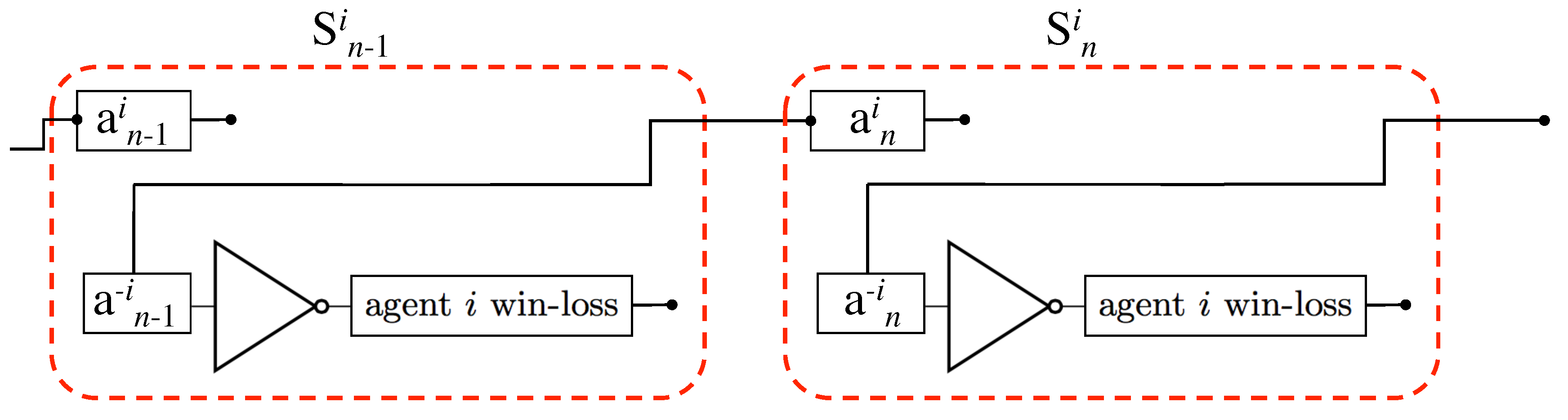
The modified Prisoner’s Dilemma game for agent i based on wins and losses using the Tit-for-Tat (TfT) strategy. and are the game states at time and n, the NOT gate is the logical operator that connects the variable to the win–loss status of the game, in this sense the NOT operator is the logic of the modified PD game. The only connection between successive game states for the TfT strategy is a direct connection between and , and neither agent i’s act nor the win–loss status of the game is in the information set of the TfT strategy. The variable influences the win–loss outcome in a similar diagram for agent just as influences the win–loss outcome for agent i in this diagram.
Figure 1.
The modified Prisoner’s Dilemma game for agent i based on wins and losses using the Tit-for-Tat (TfT) strategy. and are the game states at time and n, the NOT gate is the logical operator that connects the variable to the win–loss status of the game, in this sense the NOT operator is the logic of the modified PD game. The only connection between successive game states for the TfT strategy is a direct connection between and , and neither agent i’s act nor the win–loss status of the game is in the information set of the TfT strategy. The variable influences the win–loss outcome in a similar diagram for agent just as influences the win–loss outcome for agent i in this diagram.

Figure 2.
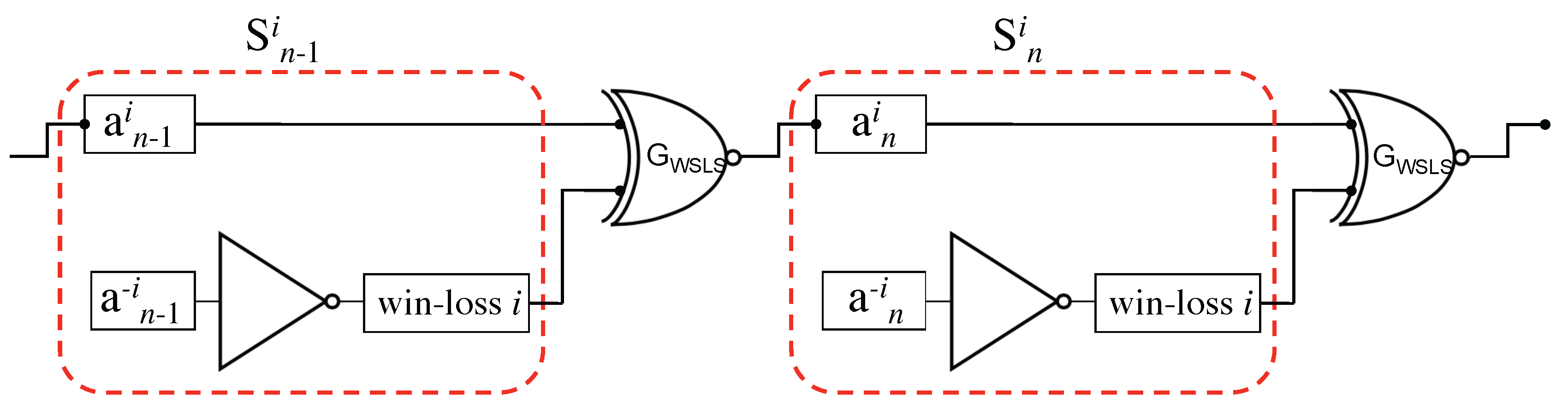
The modified Prisoner’s Dilemma game for agent i based on wins and losses and using the Win-Stay, Lose-Switch (WSLS) strategy. The WSLS strategy is equivalent to an XNOR (exclusive-nor) gate that has as its information set (inputs) win–loss} and outputs .
Figure 2.
The modified Prisoner’s Dilemma game for agent i based on wins and losses and using the Win-Stay, Lose-Switch (WSLS) strategy. The WSLS strategy is equivalent to an XNOR (exclusive-nor) gate that has as its information set (inputs) win–loss} and outputs .

Figure 3.
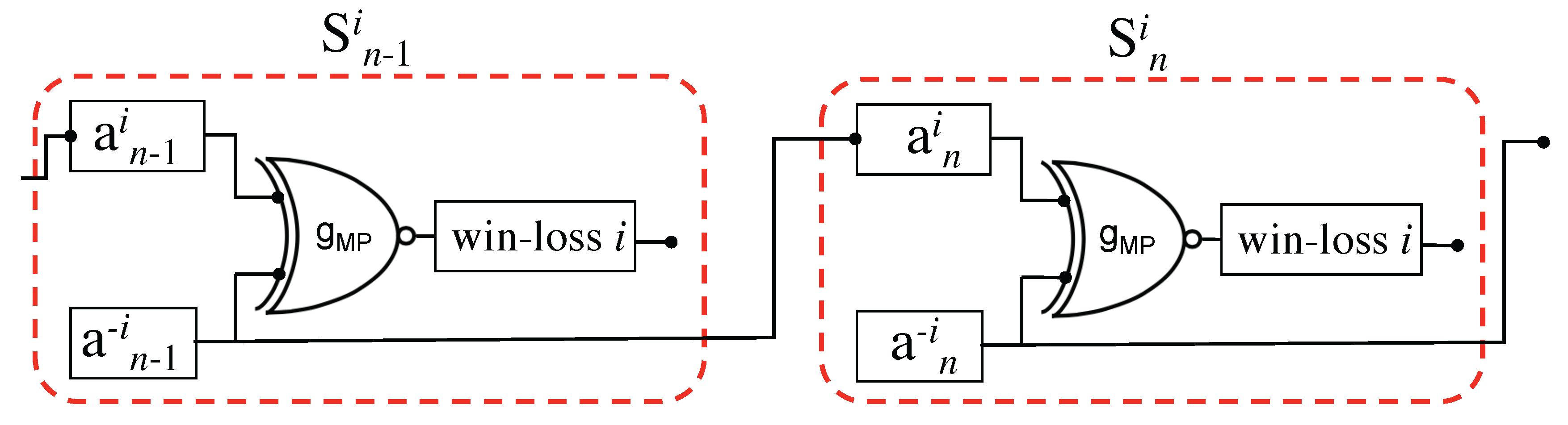
Two steps in the Matching Pennies (MP) iterated game, for agent i the elements of are related to one another via an XNOR logic gate representation of the MP game. TfT is the copy operation (identity logic gate) from to
Figure 3.
Two steps in the Matching Pennies (MP) iterated game, for agent i the elements of are related to one another via an XNOR logic gate representation of the MP game. TfT is the copy operation (identity logic gate) from to

Figure 4.
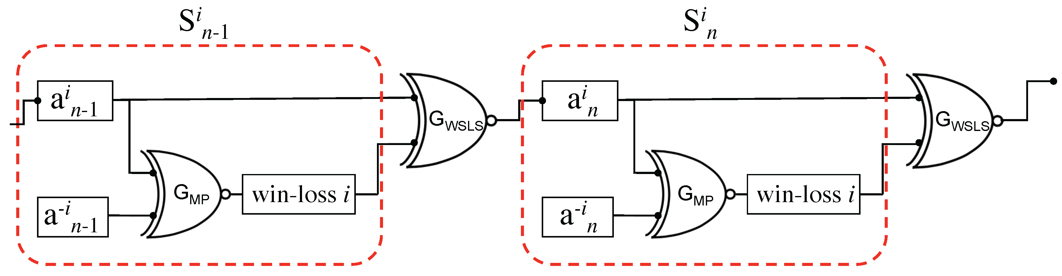
Two steps in the MP iterated game. As for Figure 3, the elements of are related to one another via an XNOR logic gate representation of the MP game. The WSLS strategy is represented as an XNOR logic gate between inputs win–loss} and output . For agent , the gate would be an XOR gate.
Figure 4.
Two steps in the MP iterated game. As for Figure 3, the elements of are related to one another via an XNOR logic gate representation of the MP game. The WSLS strategy is represented as an XNOR logic gate between inputs win–loss} and output . For agent , the gate would be an XOR gate.

Table 1.
The Prisoner’s Dilemma payoff table.
| Agent | |||
|---|---|---|---|
| Co-op | Defect | ||
| agent i | Co-op | (1 year, 1 year) | (5 years, 0 year) |
| Defect | (0 year, 5 years) | (3 years, 3 years) | |
Table 2.
Prisoner’s Dilemma as a NOT logic gate for agent i.
 | |||||
| i’s Win-Loss | WSLS | TfT | |||
| 0 (C) | 0 (c) | 1 (win) | 0 | 0 | |
| 0 (C) | 1 (d) | 0 (loss) | 1 | 1 | |
| 1 (D) | 0 (c) | 1 (win) | 1 | 0 | |
| 1 (D) | 1 (d) | 0 (loss) | 0 | 1 | |
Table 3.
Payoff table for the Matching Pennies game.
| Agent | |||
|---|---|---|---|
| Heads | Tails | ||
| agent i | Heads | ||
| Tails | |||
Table 4.
XNOR logic gate for agent i.
 | |||||
| WSLS | TfT | ||||
| 1 (H) | 1 (h) | 1 (win) | 1 | 1 | |
| 1 (H) | 0 (t) | 0 (loss) | 0 | 0 | |
| 0 (T) | 1 (h) | 0 (loss) | 1 | 1 | |
| 0 (T) | 0 (t) | 1 (win) | 0 | 0 | |
Table 5.
XOR logic gate for agent .
 | |||||
| WSLS | TfT | ||||
| 1 (H) | 1 (h) | 0 (loss) | 0 | 1 | |
| 1 (H) | 0 (t) | 1 (win) | 1 | 0 | |
| 0 (T) | 1 (h) | 1 (win) | 0 | 1 | |
| 0 (T) | 0 (t) | 0 (loss) | 1 | 0 | |
© 2017 by the author. Licensee MDPI, Basel, Switzerland. This article is an open access article distributed under the terms and conditions of the Creative Commons Attribution (CC BY) license (http://creativecommons.org/licenses/by/4.0/).
Share and Cite
MDPI and ACS Style
Harré, M. Utility, Revealed Preferences Theory, and Strategic Ambiguity in Iterated Games. Entropy 2017, 19, 201. https://doi.org/10.3390/e19050201
AMA Style
Harré M. Utility, Revealed Preferences Theory, and Strategic Ambiguity in Iterated Games. Entropy. 2017; 19(5):201. https://doi.org/10.3390/e19050201
Chicago/Turabian StyleHarré, Michael. 2017. "Utility, Revealed Preferences Theory, and Strategic Ambiguity in Iterated Games" Entropy 19, no. 5: 201. https://doi.org/10.3390/e19050201
Note that from the first issue of 2016, this journal uses article numbers instead of page numbers. See further details here.