Stochastic Stirling Engine Operating in Contact with Active Baths

Abstract

A Stirling engine made of a colloidal particle in contact with a nonequilibrium bath is considered and analyzed with the tools of stochastic energetics. We model the bath by non Gaussian persistent noise acting on the colloidal particle. Depending on the chosen definition of an isothermal transformation in this nonequilibrium setting, we find that either the energetics of the engine parallels that of its equilibrium counterpart or, in the simplest case, that it ends up being less efficient. Persistence, more than non-Gaussian effects, are responsible for this result.

1. Introduction

Every well-educated physicist has heard of Carnot or Stirling cycles. In equilibrium thermodynamics of macroscopic systems (such as a gas enclosed in some container), a cycle is a periodic sequence of transformations the system is subjected to, with a view, as far as engines are considered, extracting work from the system. For a Carnot cycle, this is the well-known adiabatic-isothermal-adiabatic-isothermal sequence, while, for a Stirling cycle, the adiabatic transformations are replaced with isochoric ones. The analysis of small, microscopic or nanoscopic systems, such as a colloidal particle in some solvent, in contrast with the nineteenth century fluid systems, poses theoretical and experimental challenges. The former have been overcome by the advent of stochastic energetics at the end of the nineties [1]. Stochastic energetics (or stochastic thermodynamics) encompass a series of concepts and methods that allow one to define work, heat, dissipation, energy, etc. at an instantaneous and fluctuating level. By taking averages, one usually recovers (with often no need to consider the limit of macroscopic systems) the standard principles of thermodynamics. The gain, however, is enormous in that stochastic energetics also allows one to quantify fluctuations, which may not be negligible for small-scale systems. An excellent review on the latest developments of stochastic thermodynamics is that by Seifert [2], while the earlier Schmiedl and Seifert paper [3] focuses specifically on the analysis of stochastic engines. Experimental realizations pose challenges of their own. These are concerned with the control of small-size objects (often by means of optical tweezers), coupled to the need to control other parameters of the experiment. The bath temperature is one of them. Another one is the optical trap stiffness that can be seen as playing a role analogous to the volume of the container enclosing the gas in the macroscopic version. The conjugate parameter (analogous to the pressure) is the particle position (squared). The first colloidal-made engines were concerned with a Stirling cycle [4,5], in which a sequence of transformations by which the bath temperature and the trap stiffness were varied was applied to the colloidal particle. This is no place to discuss what an adiabatic transformation actually means at the level of a colloidal particle in a solvent, suffice it to say that this has very recently been defined [6] and put to work in an actual Carnot cycle [7]. A lot remains to be done at the experimental level and theoretical level alike, but it is fair to say that things are pretty well-understood as far as the theoretical framework is concerned. However, a somewhat unexpected generalization of these cycles seen as transformations between equilibrium states has recently been put forward by Krishnamurthy et al. [8]. The generalization, in the spirit of the seminal work of Wu and Libchaber [9], consists of replacing the equilibrium bath by an active bath containing living bacteria in a stationary yet nonequilibrium state. The sequence of transformations thus occurs between nonequilibrium steady-states instead of between equilibrium ones. Due to the nonequilibrium nature of the bacterial bath, there is no way to define a bona fide temperature. There are, however, several ways to define an energy scale expressing the level of energetic activity of the bath (all of which reduce, under equilibrium conditions, to the physical temperature). The proposal of [8] is to use the colloid’s position fluctuations via $T_{\mathrm{act}}=\frac{k}{2}\langle x^2\rangle$ (where k is the trap stiffness). Another possibility would have been the following: in the absence of any confining force, the colloidal particle will eventually diffuse away from its initial position, so that we might then expect $\langle {(x\left(t\right)-x\left(0\right))}^2\rangle =\frac{2T}{\gamma }t$, where T is yet another acceptable active temperature (this would be the asymptotic slope in Figure 2 of [9]). One might be inclined, somewhat subjectively, to view T as better expressing the intrinsic properties of the bath, while $T_{\mathrm{act}}$ must result from a balance between the bath and some external force. We will come back to that point at a later stage.

The purpose of this work is to analyze the results of [8] in the light of a specific modeling of the bacterial bath. We argue that, in the presence of the nonequilibrium bath, the Stirling engine efficiency depends on whether T or $T_{\mathrm{act}}$ is held fixed during the isothermal transformation, a distinction which does not apply to equilibrium baths for which T and $T_{\mathrm{act}}$ are equal. Our modeling relies on a single hypothesis: the bath enters the colloid’s motion only through an extra noise term, and the noise statistics alone encode for the effect of the bath. Inspired by the suggestion of [8] that non-Gaussian statistics are essential, we will propose that the noise to which the colloid is subjected may have itself non-Gaussian statistics (recent advances of stochastic energetics for non-Gaussian but white processes [10,11] have taught us how to manipulate such signals) and possibly possess persistence properties. We will begin by a reminder of the properties of the stochastic Stirling engine between equilibrium reservoirs. We will then consider the extension to nonequilibrium bath and see how equilibrium results are not affected by choosing isothermal processes based on $T_{\mathrm{act}}$. Then, we will adopt a definition of active temperature based on the colloid’s diffusion constant and show that energy balance considerations are deeply modified and that the persistence of the noise is of key importance.

2. Stirling Cycle between Equilibrium States: A Quick Review

2.1. Modeling the Motion of a Colloidal Particle

The standard description of the dynamics of a colloidal particle in a solvent rests on a Langevin equation governing the evolution of the particle’s position $x\left(t\right)$. In the overdamped limit relevant to the description of a micron-sized particle, this Langevin equation reads

$$\gamma \frac{\mathrm{d}x}{\mathrm{d}t}=-{\partial }_{x}V+\gamma \eta ,$$

(1)

where $\gamma$ is the friction coefficient characterizing the viscous drag of the particle in the solvent (this is the inverse mobility). The external potential V depends on the particle’s position x and an external control parameter of the potential (like the stiffness of the harmonic trap). Finally, $\eta$, which, with the chosen normalization, has the dimension of a velocity, stands for a Gaussian white noise with correlations $\langle \eta \left(t\right)\eta \left(t^{\prime }\right)\rangle =\frac{2T}{\gamma }\delta (t-t^{\prime })$. Under those conditions, where the dissipation kernel exactly matches the noise correlator, as prescribed by Kubo [12], the colloidal particle is in equilibrium (provided, of course, the external potential is not time dependent). In experimental setups, the potential is harmonic and the particle’s motion is tracked in two-dimensional space, $\mathbf{r}=(x,y)$ and $V(x,k)=\frac{k}{2}(x^2+y^2)$. We will stick to a one-dimensional description for notational simplicity. In the nonequilibrium setting we want to describe here, we shall encapsulate the effects of the interactions of the colloidal particle with its nonequilibrium environment into a single ingredient, namely the noise statistics. However, there is no reason to expect the noise resulting from the interactions of the colloidal particle with the bacteria bath to be either Gaussian or white. We postpone the analysis of such active noises to the next section and now proceed with a reminder of [3,4].

2.2. Energetics of the Stirling Cycle

In this subsection, we briefly review the results presented in [4,5]. This serves as a way to set notations straight and to define the quantities of interest. A Stirling cycle $ABCDA$ is made of the following sequence of states in the stiffness-temperature space $(k,T)$:

$$A:(k_2,T_2)\stackrel{\mathrm{isothermal}}{⟶}B:(k_1,T_2)\stackrel{\mathrm{isochoric}}{⟶}C:(k_1,T_1)\stackrel{\mathrm{isothermal}}{⟶}D:(k_2,T_1)\stackrel{\mathrm{isochoric}}{⟶}A,$$

(2)

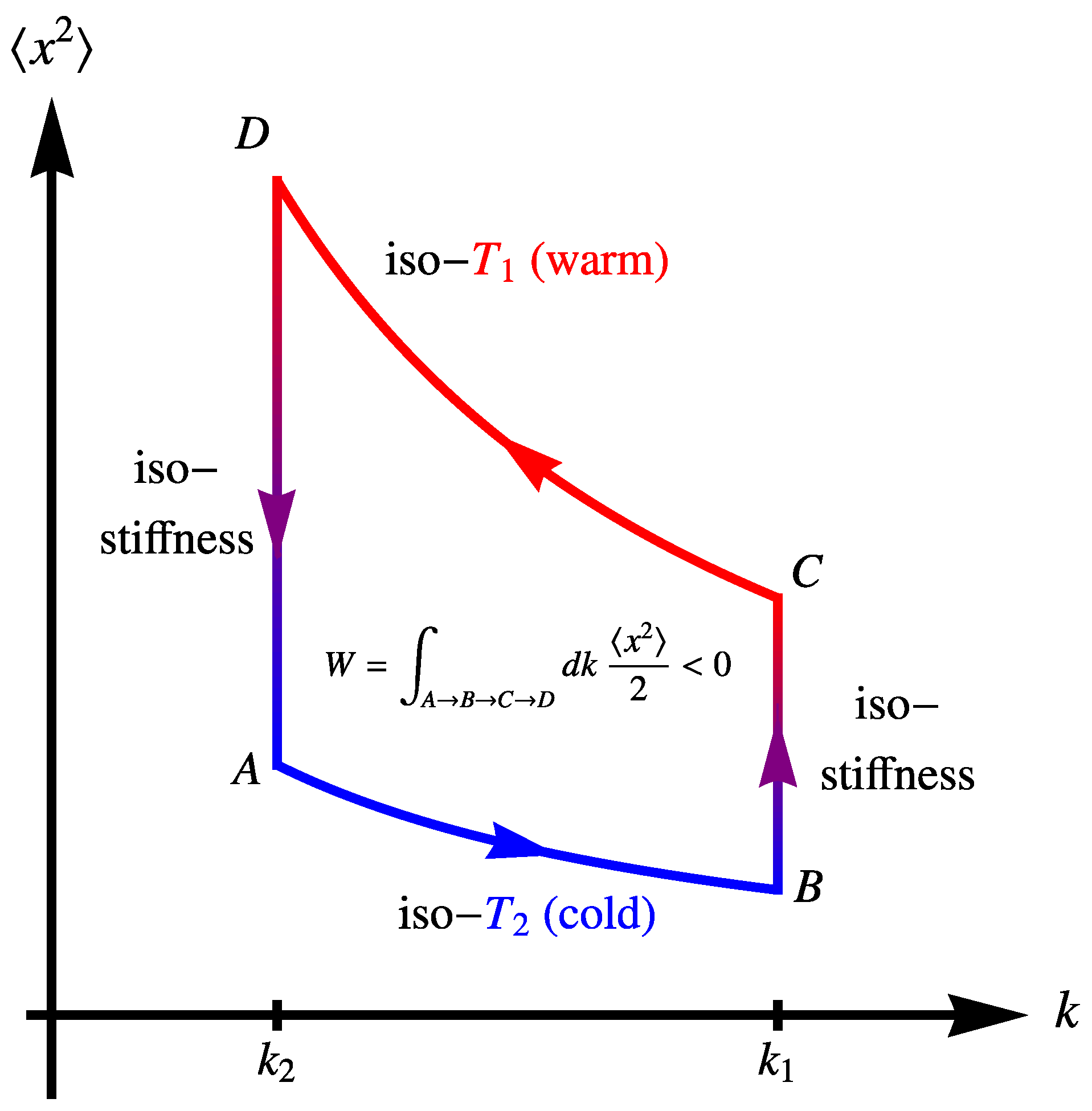
where the terminology isochoric of course refers to an iso-stiffness transformation. This cycle is sketched in Figure 1.

We will denote by $a=k_1/k_2>1$ the stiffness ratio (a large value of k is analogous to a more compressed state). The warm source is at $T_1$ while the cold source is at $T_2$ ($T_1>T_2)$. The instantaneous fluctuating energy of the particle is $V(x,k)=\frac{k}{2}{x}^2$. The work done on the colloid along a protocol driving it from state i to state f is $W={\int }_i^f\mathrm{d}t\frac{\mathrm{d}k}{\mathrm{d}t}\frac{\partial V}{\partial k}={\int }_i^f\mathrm{d}k\frac{1}{2}{x}^2$. The heat received by the colloid during the same step is given by the integral of the entropy production along the given protocol:

$$Q=-{\int }_i^f\mathrm{d}tT\sigma ,$$

(3)

where $\sigma =T^{-1}\dot{x}(\gamma \dot{x}-\gamma \eta )=-T^{-1}k\dot{x}x$ is also the rate of work performed by the particle on the bath, and thus Q is the work performed by the bath on the particle. Altogether, we thus have $Q={\int }_i^{f}kx\mathrm{d}x$. If $p_{\mathrm{eq}}\left(x\right)={\mathrm{e}}^{-k{x}^2/2T}/\sqrt{2\pi T/k}$ is the equilibrium distribution, then, up to a constant $S=-\int \mathrm{d}x{p}_{\mathrm{eq}}\left(x\right)ln{p}_{\mathrm{eq}}\left(x\right)=-\frac{1}{2}ln\frac{k}{2\pi T}+\frac{1}{2}$ is the equilibrium entropy and $\langle Q\rangle ={\int }_i^{f}T\mathrm{d}S$, with $\mathrm{d}S=-\frac{1}{2}\frac{\mathrm{d}k}{k}+\frac{1}{2}\frac{\mathrm{d}T}{T}$. This is consistent with $Q={\int }_i^{f}kx\mathrm{d}x={\left[\frac{k{x}^2}{2}\right]}_i^f-{\int }_i^f\mathrm{d}k\frac{x^2}{2}$, which is a promotion of the first law $V_f-V_i=W+Q$ to stochastic energies. Using $\langle x^2\rangle =T/k$, it is a simple exercise to determine the average heat received by the system during each step, $\langle Q_{AB}\rangle =-\frac{1}{2}{T}_{2}lna<0$, $\langle Q_{BC}\rangle =\frac{1}{2}(T_1-T_2)>0$, $\langle Q_{CD}\rangle =\frac{1}{2}{T}_{1}lna>0$ and $\langle Q_{DA}\rangle =-\frac{1}{2}(T_1-T_2)<0$. Correspondingly, $\langle W_{AB}\rangle =\frac{T_2}{2}lna$, $\langle W_{BC}\rangle =0$, $\langle W_{CD}\rangle =-\frac{T_1}{2}lna$ and $\langle W_{DA}\rangle =0$. The total average work received by the colloid is $\langle W\rangle =\langle W_{AB}+W_{CD}\rangle =-\frac{1}{2}(T_1-T_2)lna<0$. This means that the engine provides some work on average. Given that $Q_1=Q_{BC}+Q_{CD}$ and $Q_2=Q_{AB}+Q_{DA}$ are the heat effectively received by the colloid and the heat effectively given by the colloid to the bath, respectively, we define $\mathcal{E}=\frac{|\langle W\rangle |}{\langle Q_1\rangle }$ as the engine’s efficiency. The result is

$$\mathcal{E}=\frac{\langle Q_1+Q_2\rangle }{\langle Q_1\rangle }=\frac{(T_1-T_2)lna}{T_1-T_2+T_{1}lna}.$$

(4)

If a perfect regenerator was used during the isochoric cooling $D\to A,$ then the energy given out during this isochoric cooling could be used for the heating during the isochoric heating $B\to C$. Then, the heat received by the colloid would reduce to $Q_1=Q_{CD}$ and the efficiency would become ${\mathcal{E}}_C=\frac{(T_1-T_2)lna}{T_{1}lna}=1-\frac{T_2}{T_1}$ (this Carnot efficiency is of course an upper bound for $\mathcal{E}=\frac{{\mathcal{E}}_{C}lna}{{\mathcal{E}}_C+lna}$ as given in Equation (4)). Again, these results can all be found in [4]. We have now set the stage for the purpose of this work, which is to re-examine each of these steps when the colloidal particle is in contact with nonequilibrium baths just as was carried out experimentally in [8].

3. Engine Operating between Nonequilibrium Baths

3.1. Modified Langevin Equation

We stick to our hypothesis that the effects of the bacterial bath can be entirely encoded into a single random process, so that now the colloid’s position evolves according to

$$\gamma \dot{x}=-kx+\gamma {\eta }_{\mathrm{act}},$$

(5)

where the active noise ${\eta }_{\mathrm{act}}$ is a characteristic feature of the bacterial bath. Assuming this random signal inherits its properties from the bacteria making up the bath, we may expect that not only will the noise display non-Gaussian statistics, but it will also exhibit persistence properties captured by some memory kernel in the noise correlations. One way to substantiate our hypothesis on a more mathematical basis is to view the colloidal probe as interacting with the bacteria via some potential and then integrate out the degrees of freedom of the bacteria. Adapting the Vernon and Feynman approach [13] to this classical and nonequilibrium context can be seen to give rise to a dissipation kernel that depends on the bacteria-colloid interactions only, while the noise correlations (which are built from the noise felt by the bacteria themselves) in addition involve the persistence time of the bacteria. Furthermore, non-Gaussian statistics of the effective noise felt by the colloid follows directly from the non-Gaussian statistics of the noise felt by each individual active bacterium. Our approximation thus retains exactly these two features and forgets about further equilibrium-like memory effects. Among existing models, we may cite Run-and-Tumble noise, Active Brownian noise (see [14] for a review), Active Ornstein–Uhlenbeck noise [15] or even white yet non-Gaussian [10]. Following [8], we define a first active temperature $T_{\mathrm{act}}$ by the steady-state value of $x^2$: $T_{\mathrm{act}}\equiv k\langle x^2\rangle$. However, we introduce another active temperature that we denote by T by means of the colloid’s mean-square displacement in the absence of a confining force, namely, at $k=0,$ we expect that

$$\langle {(x\left(t\right)-x\left(0\right))}^2\rangle =\frac{2T}{\gamma }t$$

(6)

at large times, so that $T=\frac{\gamma }{2t}{\int }_0^t\mathrm{d}{t}_1\mathrm{d}{t}_2\langle {\eta }_{\mathrm{act}}\left(t_1\right){\eta }_{\mathrm{act}}\left(t_2\right)\rangle$. We stress that neither T nor $T_{\mathrm{act}}$ are bona fide temperatures. They merely are energy scales reflecting how the bath injects energy into the colloids. The simple fact that these temperatures may not be equal out of equilibrium highlights that these temperatures cannot be endowed with any thermodynamics meaning.

3.2. The Energetics Is Not Altered If We Use Iso-T_act Steps

Using the definition of the work $W_{i\to f}={\int }_i^f\mathrm{d}k\frac{x^2}{2},$ we see that $\langle W_{i\to f}\rangle ={\int }_i^f\mathrm{d}k\frac{T_{\mathrm{act}}}{2k},$ which leads to the exact same expressions for the work as found in the previous section, up to the replacement of the equilibrium temperature with $T_{\mathrm{act}}$. Similarly, following [2], we base our analysis on the fact that the heat is given by the work exerted by the bath on the colloid, namely, $Q_{i\to f}={\int }_i^f\mathrm{d}t\dot{x}(-\gamma \dot{x}+\gamma {\eta }_{\mathrm{act}})$, which again simplifies into $Q_{i\to f}={\int }_i^f\mathrm{d}t\dot{x}\left(kx\right)$ and thus $Q_{i\to f}={\left[\frac{k{x}^2}{2}\right]}_i^f-{\int }_i^f\mathrm{d}k\frac{x^2}{2}$. After taking averages, we are back onto the expression found in equilibrium, again up to the replacement of temperatures by the corresponding $T_{\mathrm{act}}$s. Hence, within that set of definitions and within our modeling, a quasistatic engine operating between nonequilibrium baths cannot outperform an equilibrium one. In light of the experiments of [8], this leaves us with a puzzle that we will address in the discussion section. In the following section, we suggest that perhaps another definition of the active isothermal process might lead to more striking differences with respect to an equilibrium engine.

4. Energetics Using the Diffusion Constant as an Active Temperature

In this section, we re-examine the Stirling engine operating between nonequilibrium baths using the temperature T defined in Equation (6) via the diffusion constant of an unconstrained particle. An isothermal process will now be understood as a process at constant T. Physically, this requirement is arguably more natural than processes at constant $T_{\mathrm{act}}$. Indeed, T is an intrinsic measure of the activity of the bath, which can usually be tuned easily by the experimentalist, while $T_{\mathrm{act}}$ results from a balance between the bath’s activity and a given external potential.

This new definition immediately requires us to adopt specific models for the active noise ${\eta }_{\mathrm{act}}$ because the explicit dependence of $\langle x^2\rangle$ on T and k is now of crucial importance. We examine successively the case in which ${\eta }_{\mathrm{act}}$ is a non-Gaussian but white noise, and then a persistent noise with two-point correlations exponentially decreasing in time, a case that encompasses Ornstein–Uhlenbeck noise, Run-and-Tumble or Active Brownian noise.

4.1. A Bath with White but Non-Gaussian Statistics

Let’s now assume that the active nature of the bacterial bath only surfaces through the non-Gaussian statistics of the noise ${\eta }_{\mathrm{nG}}$ appearing in the Langevin equation,

$$\gamma \dot{x}=-{\partial }_{x}V+\gamma {\eta }_{\mathrm{nG}},$$

(7)

while memory effects can be ignored in a first approximation. A non-Gaussian white noise ${\eta }_{\mathrm{nG}}\left(t\right)$ can be formed by compounding Poisson point processes with random and independent amplitudes [16]. In practice, a realization of the noise over a time interval $[0,\mathcal{T}]$ is generated by first drawing a number of points, n, from a Poisson distribution with mean $\nu \mathcal{T}$. Then, a collection of times $t_i$, with $i=1,\dots ,n$, are drawn uniformly in $[0,\mathcal{T}]$. To each $t_i$ is associated a jump amplitude $c_i$, where the $c_i$s are independent but identically distributed random variables with distribution $p\left(c\right)$. The non-Gaussian, white noise is constructed as the composition of these random-amplitude Poisson jumps:

$${\eta }_{\mathrm{nG}}\left(t\right)=\sum _i{c}_i\delta (t-t_i).$$

(8)

The generating functional of ${\eta }_{\mathrm{nG}}\left(t\right)$ is $\langle {\mathrm{e}}^{\int \mathrm{d}tj\left(t\right){\eta }_{\mathrm{nG}}\left(t\right)}\rangle ={\mathrm{e}}^{\nu \int \mathrm{d}t({\langle {\mathrm{e}}^{cj\left(t\right)}\rangle }_p-1)}$, where the p index denotes an average with respect to c and $j\left(t\right)$ is the field conjugate to ${\eta }_{\mathrm{nG}}$. The two parameters defining the noise statistics are the hitting frequency $\nu$ and the full jump distribution p. The Gaussian white noise limit is recovered as $\nu \to \infty$ and ${\langle c^2\rangle }_p\to 0$ while $\nu {\langle c^2\rangle }_p$ remains fixed. The noise has cumulants

$${\langle {\eta }_{\mathrm{nG}}\left(t_1\right)\dots {\eta }_{\mathrm{nG}}\left(t_n\right)\rangle }_{\mathrm{cumulant}}=\nu {\langle c^n\rangle }_p\delta (t_1-t_2)\dots \delta (t_{n-1}-t_n).$$

(9)

We denote by $T/\gamma =\nu {\langle c^2\rangle }_p/2$ so that $\langle {\eta }_{\mathrm{nG}}\left(t\right){\eta }_{\mathrm{nG}}\left(t^{\prime }\right)\rangle =(2T/\gamma )\delta (t-t^{\prime })$ and T matches the definition given in Equation (6). It is possible to show that, in the case of the non-Gaussian white noise, this T is actually identical to our prior definition $T_{\mathrm{act}}=\langle x^2\rangle /k$. To prove this, we start from the master equation for the probability that $x\left(t\right)$ takes the value x at time t, $P(x,t)$, which reads

$${\partial }_{t}P(x,t)={\gamma }^{-1}{\partial }_x\left(kxP(x,t)\right)+\nu \int \mathrm{d}cp\left(c\right)\left(P(x-c,t)-P(x,t)\right),$$

(10)

which we multiply by $x^2$ and integrate over x. This directly leads to

$$\begin{array}{cc}\hfill \frac{\mathrm{d}}{\mathrm{d}t}\langle x^2\rangle =& -\frac{2k}{\gamma }\langle x^2\rangle +\nu {\langle c^2\rangle }_p.\hfill \end{array}$$

(11)

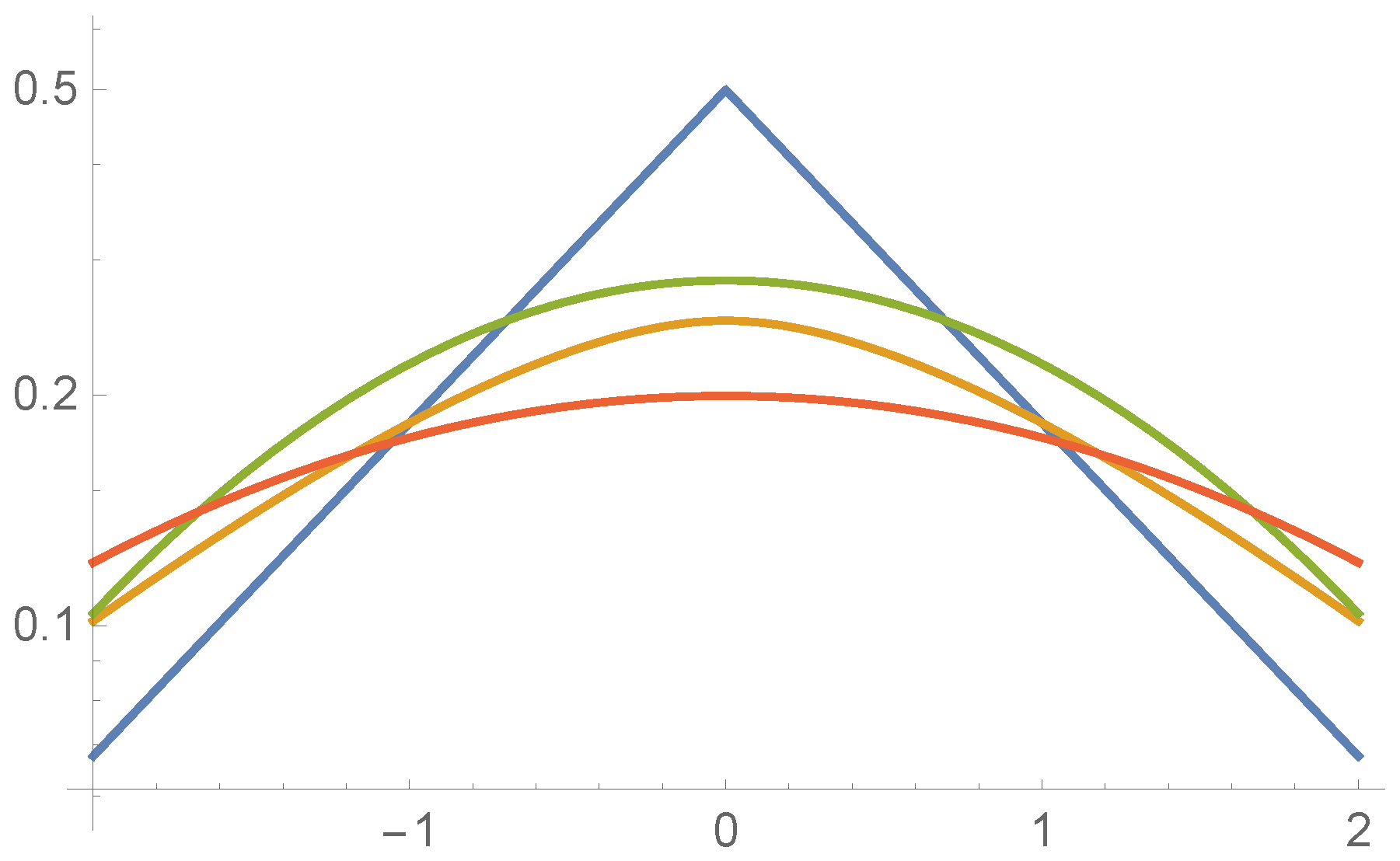
Hence, it results that in steady-state $k\langle x^2\rangle =T$, independently of the non-Gaussian noise specifics. This is an extension of equipartition to a nonequilibrium context. An identical equipartition holds for an underdamped Langevin equation with non-Gaussian noise, for which $m\dot{v}=-\gamma v-V^{\prime }+\gamma {\eta }_{\mathrm{nG}}$ leads to $m\frac{\mathrm{d}\langle v^2\rangle }{\mathrm{d}t}=-\gamma \langle v^2\rangle -\frac{\mathrm{d}}{\mathrm{d}t}\langle V\rangle +\frac{2\gamma T}{m}$. This indeed forces $\langle m{v}^2/2\rangle =T/2$ in the steady-state, irrespective of the white noise statistics. In a similar vein, one can also see that $\frac{\mathrm{d}}{\mathrm{d}t}\langle xv+\frac{\gamma }{m}\frac{x^2}{2}\rangle =\langle v^2\rangle -\frac{1}{m}\langle x{V}^{\prime }\rangle$, which leads to $\langle x{V}^{\prime }\rangle =m\langle v^2\rangle =T$ in the nonequilibrium steady-state. It immediately follows that the average works and heats will be unchanged with respect to the equilibrium discussion of Section 2.2. Note, however, that, in line with [2,10], the heat is not given anymore by the entropy production $\delta Q=-T\sigma \mathrm{d}t$ as in Equation (3). It would be an interesting task to try and evaluate the corresponding $\sigma$, which is beyond the scope of the present discussion. (This might be feasible in an expansion in the jump size a at fixed active T. Such an expansion around a Gaussian white noise is admittedly questionable in view of Pawula’s theorem [17] but can be controlled when manipulated with care [18]). Finally, that equipartition holds does not preclude strong non-Gaussian effects to show up in the colloid’s position pdf. For instance, choosing $p\left(c\right)={\mathrm{e}}^{-\left|c\right|/a}/\left(2a\right)$ (with ${\langle c^2\rangle }_p=2a^2$) for the distribution of jumps allows us to find the stationary state distribution $P_{\mathrm{ss}}\left(x\right)$. Indeed, with this choice of jump statistics [19] for $\alpha =\frac{T}{2k{a}^2}-\frac{1}{2}$ positive, we have $P_{\mathrm{ss}}\left(x\right)={C|x/a|}^{\alpha }{K}_{\alpha }\left(\right|x|/a)$ and $C=2^{-\alpha }{a}^{-1}/\left(\sqrt{\pi }\mathsf{\Gamma }(1/2+\alpha )\right)$, and thus $\langle x^2\rangle =\frac{T}{k}$ can be explicitly verified. Note $P_{\mathrm{ss}}$ exhibits a cusp at the origin for $0\le \alpha \le 1/2$, namely, for $k{a}^2<T<2k{a}^2$.

It comes as no surprise that the position statistics in the steady-state are strongly non-Gaussian as illustrated in Figure 2. However, it simply turns out that these non-Gaussian fluctuations do not interfere with the energy balance of the Stirling engine (Appendix B shows explicitly that the value of the kurtosis of the position distribution is uncorrelated from the efficiency). We now turn our attention to an active noise displaying some persistence properties with Gaussian statistics.

4.2. A Bath with a Persistent Noise

We now address more realistic modelings of the noise produced by the bacterial bath, in the form of a stochastic force imparted on the colloid that captures the persistent motion of an active particle. Such persistent noise arises from three common classes of active dynamics: Run-and-Tumble particles, active Brownian particles, and active Ornstein–Uhlenbeck motion. All three classes exhibit noise correlations that decay exponentially with a characteristic time $\tau$:

$$\langle {\eta }_{\mathrm{P}}\left(t\right){\eta }_{\mathrm{P}}\left(t^{\prime }\right)\rangle =\frac{2T}{\gamma }\times \frac{{\mathrm{e}}^{-\frac{|t-t^{\prime }|}{\tau }}}{2\tau }.$$

(12)

The prefactor T in Equation (12) matches our definition for T from Equation (6). We show in the Appendix A how the different models give rise to Equation (12) and relate T and $\tau$ to the microscopic parameters of the dynamics. Here, we adopt a unified description of the three different models by analyzing the impact of their shared noise correlator, Equation (12). Note that we restrict our discussion to one space dimension only for simplicity. In higher dimensions, the correlator of each component of the (vectorial) noise is still given by Equation (12), and, by symmetry, our results trivially generalize to a spherically harmonic potential.

If we interpret the isothermal transformations of Figure 1 as iso-T processes (as opposed to iso-$T_{\mathrm{act}}$), the energetics of our Stirling cycle now differ from the equilibrium analysis of Section 2.2. During an iso-T protocol, $\langle x^2\rangle$ does not trace an isotherm with the form $\langle x^2\rangle \propto k^{-1}$. The new form of the isotherm depends only on the two-point correlator $\langle {\eta }_{\mathrm{P}}\left(t\right){\eta }_{\mathrm{P}}\left(t^{\prime }\right)\rangle$ and not on higher-order correlations, allowing us to simultaneously treat all three types of active motion. Indeed, in Fourier space, Equation (7) reads

$$(k+i\gamma \omega )\tilde{x}\left(\omega \right)=\gamma {\tilde{\eta }}_{\mathrm{P}}\left(\omega \right),$$

(13)

with the Fourier transform defined as $\tilde{f}\left(\omega \right)={\int }_{-\infty }^{+\infty }f\left(t\right)e^{-i\omega t}\mathrm{d}t$. One can then show that in steady state

$$\langle x^2\rangle ={\int }_{-\infty }^{+\infty }\frac{\mathrm{d}\omega }{2\pi }\frac{{\gamma }^2\langle {\tilde{\eta }}_{\mathrm{P}}\left(\omega \right){\tilde{\eta }}_{\mathrm{P}}(-\omega )\rangle }{k^2+{\omega }^2{\gamma }^2}.$$

(14)

For the noise correlator Equation (12), $\langle {\tilde{\eta }}_{\mathrm{P}}\left(\omega \right){\tilde{\eta }}_{\mathrm{P}}(-\omega )\rangle =2T/\left(\gamma (1+{\tau }^2{\omega }^2)\right)$ so that we obtain

$$\langle x^2\rangle =\frac{T}{k(1+k\tau /\gamma )}.$$

(15)

In the notation of Section 3.1, $T_{\mathrm{act}}\equiv k\langle x^2\rangle =T/(1+\mathsf{\Omega }\tau ),$ where we have defined the frequency $\mathsf{\Omega }\equiv k/\gamma$.

Let us proceed, then, with the cycle Equation (2) in which we consider isothermal processes at fixed T. The average work has the expression $\langle W_{i\to f}\rangle =\frac{1}{2}{\int }_i^f\mathrm{d}k\frac{T}{k(1+\mathsf{\Omega }\tau )}$, which is zero along an isochoric protocol, but which now reads $\langle W_{i\to f}\rangle =\frac{T}{2}{[ln\frac{k}{1+\mathsf{\Omega }\tau }]}_i^f$ along an iso-T protocol. Similarly, the average heat reads $\langle Q_{i\to f}\rangle ={\left[\frac{T/2}{1+\mathsf{\Omega }\tau }\right]}_i^f-\frac{1}{2}{\int }_i^f\mathrm{d}k\frac{T}{k(1+\mathsf{\Omega }\tau )}$. Putting everything together, we find

$$\begin{array}{cc}\hfill \langle Q_{AB}\rangle & =\frac{T_2}{2}\left[\frac{1}{1+{\mathsf{\Omega }}_1\tau }-\frac{1}{1+{\mathsf{\Omega }}_2\tau }\right]-\frac{T_2}{2}ln\left[a\frac{1+{\mathsf{\Omega }}_2\tau }{1+{\mathsf{\Omega }}_1\tau }\right],\hfill \\ \hfill \langle Q_{BC}\rangle & =\frac{(T_1-T_2)/2}{1+{\mathsf{\Omega }}_1\tau }>0,\hfill \\ \hfill \langle Q_{CD}\rangle & =\frac{T_1}{2}\left[\frac{1}{1+{\mathsf{\Omega }}_2\tau }-\frac{1}{1+{\mathsf{\Omega }}_1\tau }\right]+\frac{T_1}{2}ln\left[a\frac{1+{\mathsf{\Omega }}_2\tau }{1+{\mathsf{\Omega }}_1\tau }\right],\hfill \\ \hfill \langle Q_{DA}\rangle & =-\frac{(T_1-T_2)/2}{1+{\mathsf{\Omega }}_2\tau }<0,\hfill \end{array}$$

(16)

while the average works are given by

$$\langle W_{AB}\rangle =\frac{T_2}{2}lna\frac{1+{\mathsf{\Omega }}_2\tau }{1+{\mathsf{\Omega }}_1\tau },\langle W_{CD}\rangle =-\frac{T_1}{2}lna\frac{1+{\mathsf{\Omega }}_2\tau }{1+{\mathsf{\Omega }}_1\tau },\langle W_{BC}\rangle =\langle W_{DA}\rangle =0,$$

(17)

and thus $\mathcal{E}=\frac{-\langle W\rangle }{\langle Q_{BC}+Q_{CD}\rangle }$ in the $T_1\gg T_2$ limit is

$${\mathcal{E}}_{\mathrm{sat}}=\frac{lna\frac{1+{\mathsf{\Omega }}_2\tau }{1+{\mathsf{\Omega }}_1\tau }}{lna\frac{1+{\mathsf{\Omega }}_2\tau }{1+{\mathsf{\Omega }}_1\tau }+\frac{1}{1+{\mathsf{\Omega }}_2\tau }}.$$

(18)

In the limit of small correlation time (${\mathsf{\Omega }}_1\tau \ll 1$), we find that

$${\mathcal{E}}_{\mathrm{sat}}\simeq \frac{lna}{1+lna}-{\mathsf{\Omega }}_2\tau \frac{a-1-lna}{{(1+lna)}^2}+\mathcal{O}\left({\tau }^2\right).$$

(19)

In Equation (19), the correction to ${\mathcal{E}}_{\mathrm{sat}}$ actually remains negative at arbitrary values of $\tau$: the efficiency saturates to a lower value due to the persistent properties of the noise when compared to equilibrium (no persistence). The cost of maintaining nonequilibrium steady-state is not paid off by an improved efficiency! While the available work has increased, the required energy to operate the engine has increased by an even larger amount.

Let us stress here that the generality of these results, which depend only on the two-point correlator of the noise but not on higher-order statistics, can seem rather surprising because the behavior of active Ornstein–Uhlenbeck, Run-and-Tumble and Active Brownian particles in an harmonic trap are all qualitatively different. The case of an active Ornstein–Uhlenbeck noise in a quadratic potential is special in that the colloidal particle actually is in equilibrium [15]. The equilibrium distribution is $p_{\mathrm{eq}}\left(x\right)\sim {\mathrm{e}}^{-\frac{k(1+\mathsf{\Omega }\tau )}{2T}{x}^2}$ (whether and how this extends beyond a quadratic potential was discussed in [20]), from which $T_{\mathrm{act}}=T/(1+\mathsf{\Omega }\tau )$ is readily extracted. On the contrary, Active Brownian and Run-and-Tumble particles have a richer (nonequilibrium) physics. In particular, if the particle is persistent on a time scale larger than ${\mathsf{\Omega }}^{-1}$, the steady-state distribution is not peaked around $x=0$ (the particle spends most of its time on the edge of the trap) [14]. It is therefore surprising that these differences do not affect the thermodynamics of our engine.

4.3. A Bath Described by a More General Langevin Equation

A more general description of the effect of the bath on the colloidal particle includes memory effect in the dissipation as well, as discussed by Berthier and Kurchan [21] in a different context. One obtains a Langevin equation of the form

$$\gamma {\int }_{-\infty }^t\mathrm{d}{t}^{\prime }{K}_{\mathrm{diss}}(t-t^{\prime })\dot{x}\left(t^{\prime }\right)=-kx+\gamma \eta ;\langle \eta \left(t\right)\eta \left(t^{\prime }\right)\rangle =\frac{2T}{\gamma }{K}_{\mathrm{inj}}\left(\right|t-t^{\prime }\left|\right)$$

(20)

with generic injection and dissipation kernels $K_{\mathrm{inj}}$ and $K_{\mathrm{diss}}$. Equilibrium is achieved on condition that $K_{\mathrm{inj}}\left(\omega \right)$ and $\mathrm{Re}{K}_{\mathrm{diss}}\left(\omega \right)$ are equal. The ratio

$$T_{\mathrm{eff}}\left(\omega \right)=T\frac{K_{\mathrm{inj}}\left(\omega \right)}{\mathrm{Re}{K}_{\mathrm{diss}}\left(\omega \right)}$$

(21)

tells us about the mismatch between injection and dissipation. In the cases considered previously, with $K_{\mathrm{diss}}\left(\omega \right)=1$, we ended up with $T_{\mathrm{eff}}\left(\omega \right)=\frac{T}{1+{\left(\omega \tau \right)}^2}$. The characteristic frequency of the relaxation within the harmonic well being $\mathsf{\Omega }$, we a posteriori understand that in the regime where persistence matters, namely, when $\mathsf{\Omega }\tau \gg 1$, $T_{\mathrm{eff}}(\omega >\mathsf{\Omega })\to 0$, and thus the position spectrum will be cut-off beyond $\omega =\mathsf{\Omega }$. It is thus no surprise that eventually $\langle x^2\rangle <T/k$, or $T_{\mathrm{act}}<T$. Of course, in the presence of a more complicated dissipation kernel $K_{\mathrm{diss}}$, the latter inequality can be challenged. Should one devise a dissipation kernel such that $T_{\mathrm{act}}>T$, one might reasonably suspect that the thermodynamic efficiency could exceed that of the equilibrium Stirling engine.

Let us therefore consider how the energetics of the cycle in Figure 1 are impacted by the relationship between $T_{\mathrm{act}}$ and T. In particular, we repeat the analysis of Section 4.2 by assuming $T_{\mathrm{act}}=Tf\left(k\right)$ for a generic function f. The derivation proceeds exactly as before and we obtain for the heat and work on each segment

$$\begin{array}{c}\hfill \langle W_{AB}\rangle =\frac{T_2}{2}\left[G\left(k_1\right)-G\left(k_2\right)\right];\langle W_{CD}\rangle =-\frac{T_1}{2}\left[G\left(k_1\right)-G\left(k_2\right)\right];\langle W_{BC}\rangle =\langle W_{DA}\rangle =0;\end{array}$$

(22)

$$\begin{array}{c}\hfill \langle Q_{AB}\rangle =-\frac{T_2}{2}\left[G\left(k_1\right)-G\left(k_2\right)\right]+\frac{T_2}{2}\left[f\left(k_1\right)-f\left(k_2\right)\right];\langle Q_{BC}\rangle =\frac{(T_1-T_2)}{2}f\left(k_1\right);\end{array}$$

(23)

$$\begin{array}{c}\hfill \langle Q_{CD}\rangle =\frac{T_1}{2}\left[G\left(k_1\right)-G\left(k_2\right)\right]-\frac{T_1}{2}\left[f\left(k_1\right)-f\left(k_2\right)\right];\langle Q_{DA}\rangle =\frac{(T_2-T_1)}{2}f\left(k_2\right);\end{array}$$

(24)

where $G\left(k\right)$ is defined such that $G^{\prime }=f/k$. The maximum efficiency in the limit $T_1\gg T_2$ then reads

$${\mathcal{E}}_{\mathrm{sat}}=\frac{G\left(k_1\right)-G\left(k_2\right)}{f\left(k_1\right)+G\left(k_1\right)-G\left(k_2\right)}.$$

(25)

This leads to the simple criterion that, in this limit, the cycle outperforms an equilibrium Stirling engine if and only if

$${\int }_{k_2}^{k_1}\frac{f\left(k\right)}{kf\left(k_1\right)}\mathrm{d}k>{\int }_{k_2}^{k_1}\frac{\mathrm{d}k}{k}.$$

(26)

In particular, if $f\left(k\right)$ is an increasing function of k in the range $[k_2;k_1]$, the active engine outperforms the equilibrium one. This could correspond to a physical situation in which energy injection happens at a particular, finite length scale. As an example, a semi-flexible filament immersed in a bath of Active Brownian particles is excited at a characteristic length scale [22] and could thus be a candidate to realize such an efficient engine.

5. Discussion: Back to Experiments

We have assumed all along that the tagged colloidal particle is subjected to a noise that inherits its properties from those of the bath while the rest of its dynamics are unchanged. That the effect of the nonequilibrium bath can be encoded in a single random signal as an extra force does not seem to be an outrageous hypothesis, though, given the size of the bacteria used in [8], comparable to that of the colloidal particle, perhaps hydrodynamic effects should be taken into account, as well as further memory effects (in the dissipation kernel and in noise correlations). Within that framework, we might anticipate that bacteria in a constant temperature medium maintain a fixed activity, and thus the statistical properties of the random forces should remain unchanged throughout the isothermal transformation. However, because the random forces do not emerge from equilibrium thermal fluctuations, there is not a unique way to characterize which aspect of the random forces remains constant. We have shown that, with a definition of the isothermal process based on a iso-“potential energy”, we see no reason for the equilibrium results to be altered in any way. Coming back to [8], aside from the limiting efficiency in the high $T_1\gg T_2$ limit, our theoretical observation is altogether rather consistent with the experiments.

It is interesting to consider how the nonequilibrium nature of the baths could result in an engine efficiency that differs from the equilibrium efficiency. To this end, we have suggested an alternative definition of an isothermal process in which the active temperature is defined through the diffusion constant of a particle without any external potential. With this definition, in stark contrast to the iso-”potential energy” definition, the efficiency of a Stirling engine takes a dramatically different form that involves the persistence time of the noise produced by the bacteria. Interestingly, we are able to pinpoint memory effects as being responsible for the deviation from equilibrium-like efficiencies. Non-Gaussian statistics alone is not a sufficient ingredient (we have shown equipartition to hold in the limiting non-Gaussian but white scenario).

From an experimental standpoint, achieving an isothermal process defined through the diffusion constant certainly involves working at constant ambient temperature. However, it also involves working at constant activity for the bacteria. The latter are eventually propelled by molecular motors which consume ATP (which should therefore be in sufficient amounts). In other words, food for the bacteria must remain at a constant level (and the bacteria population as well). The former, namely the ambient temperature, controls the chemical kinetics behind the active processes actually propelling the bacteria. Lowering the ambient temperature will affect the kinetics of the bacteria and will lead to a decreased diffusion constant. Whether and how the persistence time of the bacteria’s motion is affected is, in our view, an interesting and challenging question beyond the scope of the present work. An alternative way to vary the diffusion constant might be to vary food concentration.

We hope the suggestion to use our alternative active temperature will trigger further experiments along the lines of [8].

References

- Sekimoto, K. Stochastic Energetics; Lecture Notes in Physics; Springer: Berlin/Heidelberg, Germany, 2010. [Google Scholar]
- Seifert, U. Stochastic thermodynamics, fluctuation theorems and molecular machines. Rep. Prog. Phys. 2012, 75, 126001. [Google Scholar] [CrossRef] [PubMed]
- Schmiedl, T.; Seifert, U. Efficiency at maximum power: An analytically solvable model for stochastic heat engines. Eur. Lett. 2008, 81, 20003. [Google Scholar] [CrossRef]
- Blickle, V.; Bechinger, C. Realization of a micrometre-sized stochastic heat engine. Nat. Phys. 2011, 8, 143–146. [Google Scholar] [CrossRef]
- Horowitz, J.M.; Parrondo, J.M.R. Thermodynamics: A Stirling effort. Nat. Phys. 2012, 8, 108–109. [Google Scholar] [CrossRef]
- Martínez, I.A.; Roldán, E.; Dinis, L.; Petrov, D.; Rica, R.A. Adiabatic Processes Realized with a Trapped Brownian Particle. Phys. Rev. Lett. 2015, 114, 120601. [Google Scholar] [CrossRef] [PubMed]
- Martinez, I.A.; Roldan, E.; Dinis, L.; Petrov, D.; Parrondo, J.M.R.; Rica, R.A. Brownian Carnot engine. Nat. Phys. 2016, 12, 67–70. [Google Scholar] [CrossRef] [PubMed]
- Krishnamurthy, S.; Ghosh, S.; Chatterji, D.; Ganapathy, R.; Sood, A.K. A micrometre-sized heat engine operating between bacterial reservoirs. Nat. Phys. 2016, 12, 1134–1138. [Google Scholar] [CrossRef]
- Wu, X.L.; Libchaber, A. Particle Diffusion in a Quasi-Two-Dimensional Bacterial Bath. Phys. Rev. Lett. 2000, 84, 3017–3020. [Google Scholar] [CrossRef] [PubMed]
- Kanazawa, K.; Sagawa, T.; Hayakawa, H. Stochastic Energetics for Non-Gaussian Processes. Phys. Rev. Lett. 2012, 108, 210601. [Google Scholar] [CrossRef] [PubMed]
- Kanazawa, K.; Sagawa, T.; Hayakawa, H. Heat conduction induced by non-Gaussian athermal fluctuations. Phys. Rev. E 2013, 87, 052124. [Google Scholar] [CrossRef] [PubMed]
- Kubo, R. The fluctuation-dissipation theorem. Rep. Prog. Phys. 1966, 29, 255. [Google Scholar] [CrossRef]
- Feynman, R.P.; Vernon, F.L. The theory of a general quantum system interacting with a linear dissipative system. Ann. Phys. 1963, 24, 118–173. [Google Scholar] [CrossRef]
- Solon, A.; Cates, M.; Tailleur, J. Active brownian particles and run-and-tumble particles: A comparative study. Eur. Phys. J. Spec. Top. 2015, 224, 1231–1262. [Google Scholar] [CrossRef]
- Szamel, G. Self-propelled particle in an external potential: Existence of an effective temperature. Phys. Rev. E 2014, 90, 012111. [Google Scholar] [CrossRef] [PubMed]
- Van Kampen, N. Stochastic Processes in Physics and Chemistry; Elsevier: Amsterdam, The Netherlands, 1992; Volume 1. [Google Scholar]
- Pawula, R. Generalizations and extensions of the Fokker–Planck–Kolmogorov equations. IEEE Trans. Inf. Theory 1967, 13, 33–41. [Google Scholar] [CrossRef]
- Popescu, D.M.; Lipan, O. A Kramers-Moyal Approach to the Analysis of Third-Order Noise with Applications in Option Valuation. PLoS ONE 2015, 10, e0116752. [Google Scholar] [CrossRef] [PubMed]
- Fodor, E.H.; Hayakawa, J.T.; van Wijland, F. What is the role of non Gaussian noise in assemblies of self-propelled active particles? in preparation.
- Fodor, É.; Nardini, C.; Cates, M.E.; Tailleur, J.; Visco, P.; van Wijland, F. How far from equilibrium is active matter? Phys. Rev. Lett. 2016, 117, 038103. [Google Scholar] [CrossRef] [PubMed]
- Berthier, L.; Kurchan, J. Non-equilibrium glass transitions in driven and active matter. Nat. Phys. 2013, 9, 310–314. [Google Scholar] [CrossRef]
- Nikola, N.; Solon, A.P.; Kafri, Y.; Kardar, M.; Tailleur, J.; Voituriez, R. Active Particles with Soft and Curved Walls: Equation of State, Ratchets, and Instabilities. Phys. Rev. Lett. 2016, 117, 098001. [Google Scholar] [CrossRef] [PubMed]
- Tailleur, J.; Cates, M.E. Sedimentation, trapping, and rectification of dilute bacteria. Eur. Lett. 2009, 86, 60002. [Google Scholar] [CrossRef]
Figure 1.
Schematic diagram of the Stirling cycle in stiffness-position space. Unlike its thermodynamic counterpart, the cycle is run counter-clockwise but is nevertheless an engine cycle.
Figure 2.
Log of the probability of the colloid’s position as a function of position (for a unit a), in equilibrium with Gaussian statistics (red at , green at ) or out of equilibrium as given by (blue at , orange at ).
© 2017 by the authors. Licensee MDPI, Basel, Switzerland. This article is an open access article distributed under the terms and conditions of the Creative Commons Attribution (CC BY) license (http://creativecommons.org/licenses/by/4.0/).
Share and Cite
MDPI and ACS Style
Zakine, R.; Solon, A.; Gingrich, T.; Van Wijland, F. Stochastic Stirling Engine Operating in Contact with Active Baths. Entropy 2017, 19, 193. https://doi.org/10.3390/e19050193
AMA Style
Zakine R, Solon A, Gingrich T, Van Wijland F. Stochastic Stirling Engine Operating in Contact with Active Baths. Entropy. 2017; 19(5):193. https://doi.org/10.3390/e19050193
Chicago/Turabian StyleZakine, Ruben, Alexandre Solon, Todd Gingrich, and Frédéric Van Wijland. 2017. "Stochastic Stirling Engine Operating in Contact with Active Baths" Entropy 19, no. 5: 193. https://doi.org/10.3390/e19050193
Note that from the first issue of 2016, this journal uses article numbers instead of page numbers. See further details here.