
A Distribution Family Bridging the Gaussian and the Laplace Laws, Gram–Charlier Expansions, Kurtosis Behaviour, and Entropy Features

Dipartimento di Discipline matematiche, Finanza matematica ed Econometria, Università Cattolica del Sacro Cuore, Largo Gemelli 1, 20123 Milano, Italy
*
Author to whom correspondence should be addressed.
Entropy 2017, 19(4), 149; https://doi.org/10.3390/e19040149
Submission received: 10 February 2017
/
Revised: 24 March 2017
/
Accepted: 28 March 2017
/
Published: 31 March 2017
Abstract
:The paper devises a family of leptokurtic bell-shaped distributions which is based on the hyperbolic secant raised to a positive power, and bridges the Laplace and Gaussian laws on asymptotic arguments. Moment and cumulant generating functions are then derived and represented in terms of polygamma functions. The behaviour of shape parameters, namely kurtosis and entropy, is investigated. In addition, Gram–Charlier-type (GCT) expansions, based on the aforementioned distributions and their orthogonal polynomials, are specified, and an operational criterion is provided to meet modelling requirements in a possibly severe kurtosis and skewness environment. The role played by entropy within the kurtosis ranges of GCT expansions is also examined.
Keywords:
power-raised hyperbolic secant distributions; limit laws; kurtosis; skewness; entropy; Gram–Charlier-type expansionsMSC2010:
primary 60E05; secondary 94A17; 60E99; 62H10; 33EXX1. Introduction
The paper specifies the family of power-raised hyperbolic secant (PHS) distributions obtained by raising the hyperbolic secant function to an arbitrary positive power n, duly normalized.
Moment-generating functions arise directly from a classical integral representation of Euler’s Beta function, clearing the way for closed-form expressions of cumulants and moments in terms of polygamma functions. In particular, the kurtosis varies with n within a range of values, bounded by 6, from above, and by 3, from below, as n tends to 0 and to ∞, respectively.
The PHS family includes the hyperbolic secant and the logistic laws as special cases by taking n = 1 and n = 2, respectively. Both distributions have been widely investigated and variously generalized in the literature (see, e.g., [1,2,3,4]). The PHS family is not meant to be one of such generalizations, and is devised to encompass a whole category of bell-shaped distributions whose moment characterizations paves the way to wide-ranging extensions in the form of Gram–Charlier-type (GCT) expansions.
Leptokurtosis turns out to be inherent in these distributions, insofar as their limit laws prove to correspond to the Laplace and Gaussian densities, on asymptotic arguments, as n → 0 and n → ∞, respectively.
The behaviour of shape parameters, namely kurtosis and entropy, is examined from a specular standpoint.
It results that simple PHS specifications can be unsuitable to deal with severe kurtosis. However, as the paper shows, this hurdle can, nonetheless, be largely overcome. This is achieved by moving from PHS distributions to GCT expansions, using an argument similar to that used to alter the moments of a Gaussian via a Gram–Charlier series (see, e.g., [5] and more recently [6]). A first approach to the issue, with reference to logistic and hyperbolic secant laws, can be found in [7].
For an arbitrary PHS density, the paper specifies a GCT expansion based on the fourth and third degree polynomials associated with the parent density—making allowances for extra-kurtosis and skewness as required.
Both the feasible set of kurtosis values and the feasible region in the kurtosis-skewness plane, for which the aforementioned GCT expansions are positive definite functions are ascertained by algebraic argument. The admissible values of kurtosis span the range 3–24. As for asymmetry, the opportunity set crucially depends on the extra-kurtosis with the absolute skewness possibly attaining values around one.
The behaviour of entropy within the ranges of values taken by kurtosis of GCT expansions is investigated and some light is shed on their dual role as shape parameters.
The characteristics of the power-raised hyperbolic secant family of distributions and their GCT expansions prove useful in several contexts, such as financial time series analysis, where there is evidence of possibly severe leptokurtosis.
For practical purposes and possible applications of the analytic toolkit here developed, a (reverse) sigmoid curve is envisaged across the domain of GCT positive definiteness in the plane of the kurtosis vs. the PHS exponent, thus establishing a one-to-one correspondence between a given kurtosis level and the parent PHS density of the intended GCT expansion. Still looking at possible application requirements, it should be pointed out that, for levels of kurtosis within the range 5–21, the GCT expansions so obtained also allow for significant asymmetry, the admissible absolute skewness resulting being >0.8.
The paper is organized as follows: The power-raised hyperbolic secant distributions are introduced in Section 2, and their moments, kurtosis, and limit laws established. The issue of entropy in PHS distributions is addressed in Section 3. Section 4 specifies GCT expansions of the aforementioned distributions. The positive-definiteness requirement on excess-kurtosis and skewness are established on precise algebraic arguments, and the opportunity sets for kurtosis and skewness determined accordingly. Section 5 sheds light on the behaviour of entropy within the admissible kurtosis ranges of GCT expansions. Section 6 provides an operational criterion which permits the selection of an appropriate parent PHS density and GCT expansion to tailor to excess-kurtosis and skewness evidence. A few concluding remarks complete the article.
2. A Family of Distributions
Let us first establish the following:
Theorem 1.
Consider the family of functions:
Let:
where B(.,.) is the Euler Beta function. Then, the expression:
where is written for , defines the family of the power raised hyperbolic secant (PHS) distributions whose even moments:
obey the recursion rule:
where is the polygamma function of order i.
Proof.
See Appendix A.
As the effect of standardization is to multiply the cumulants (see Equation (A8) in Appendix A):
by (see, e.g., [5]), the moments of will be modified accordingly, yielding the reduced moments .
In particular, measures the kurtosis .
In this connection we have the following.
Theorem 2.
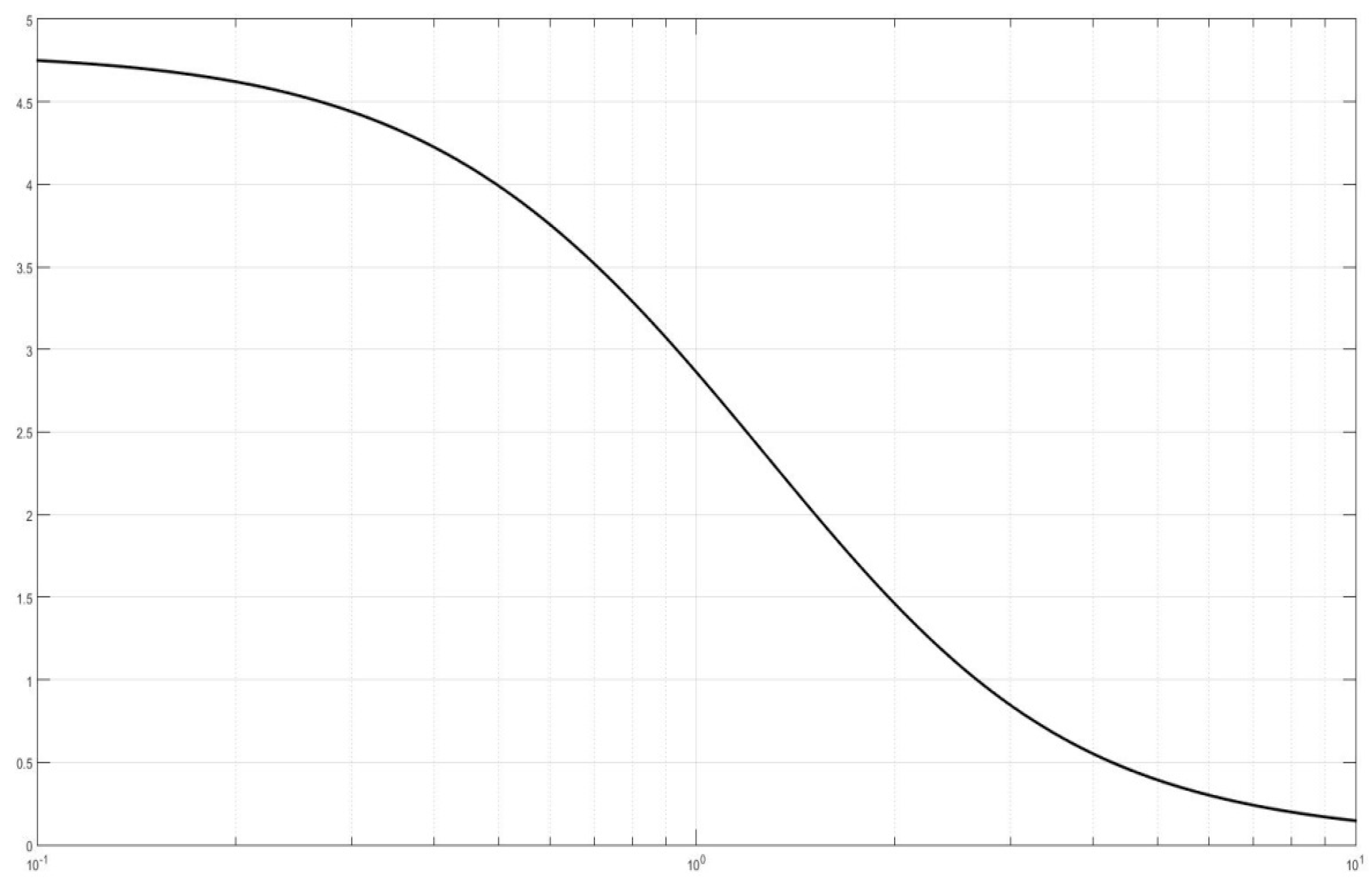
The PHS distributions Equation (3) are leptokurtic. The kurtosis is given by:
The following properties of :
prove true.
Proof.
See Appendix A.
Figure 1 shows the behaviour of the index as n varies from 0.1 to 10.
In fact, the asymptotic implications of PHS functions, far from being confined to kurtosis, are essential from the distribution stand-point as the following theorem proves. The latter shows that the family of PHS distributions bridges the Laplace and Gaussian laws.
Theorem 3.
The standardized PHS density functions specified as follows (see proof of Theorem 1 in Appendix A)
enjoy the following limit properties,
- (i)
- approaches the normed Laplace law as n → 0, that is
- (ii)
- approaches the standard Gaussian law as n → ∞, that is
Proof.
See Appendix A.
3. Entropy vs. Kurtosis of Power-Raised Hyperbolic Secant Distributions
The entropy of an absolutely continuous distribution with density function is given by the integral:
where use is made of natural logarithms for convenience. The entropy from Equation (13) assumes its largest value in the case of a normal distribution (see [8], pp. 367–368).
Simple computations show that:
The Gaussian and Laplace distributions, being the limits as n → 0 and as n → ∞ respectively, of the PHS family of distributions, the more general question of the values taken by as n moves from 0 to ∞ naturally arises. In this connection we have the following
Theorem 4.
The entropy of the PHS distribution family is given by:
with and b given by Equations (10) and (A11) in Appendix A, respectively.
Proof.
See Appendix A.
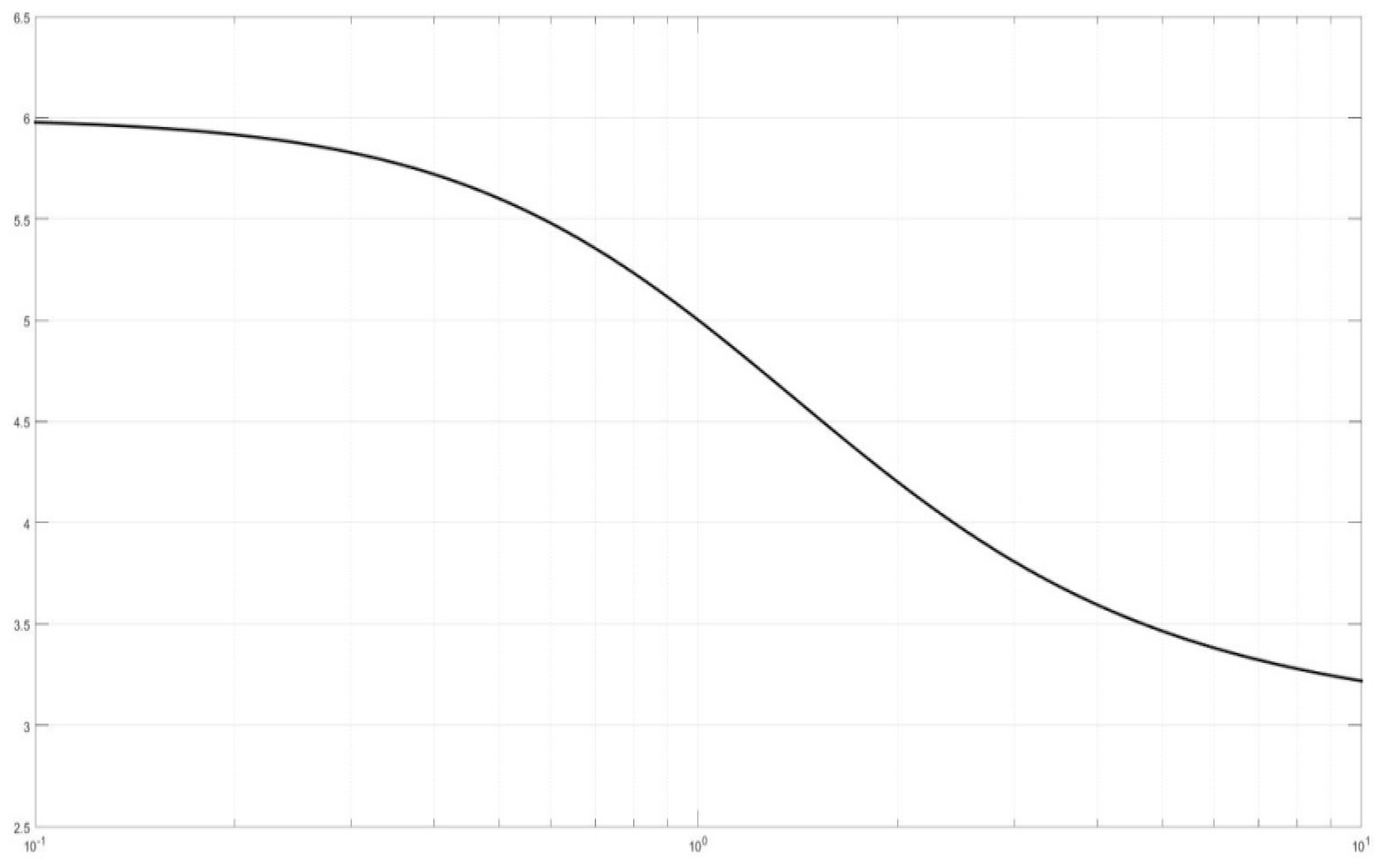
The following graph shows the behaviour of the entropy as n varies from 0.1 to 10.
Inspecting Figure 2 above and Figure 1 of Section 2, we note how the entropy is an increasing function of n (see Figure 2), whereas the kurtosis K is a decreasing function of n (see Figure 1).
Thus, as far as PHS distributions are concerned, a drop in entropy, as compared with the Gaussian case, is accompanied by leptokurtosis, and vice versa. Consequently, for this family of distributions, an entropy loss is an indicator of excess kurtosis.
4. GCT Expansions of PHS Distributions
In this section we conceive a GCT expansion of PHS distributions by assigning to the fourth degree polynomial orthogonal with respect to in Equation (10) the role once played by the fourth degree Hermite polynomial (see, e.g., [9], p. 28). The following GCT expansion shaped on extra-kurtosis β, is specified as:
where is the fourth-degree monic polynomial, orthogonal with respect to the density function , is the squared norm of the aforementioned polynomial, and β is a shape parameter subject to being positive definite.
As a by-product of Theorem 3, p(x,0) and p(x,∞), respectively, turn out to be the Laguerre and Hermite polynomials. More generally, (see, e.g., [10,11]), the monic polynomial orthogonal with respect to the function can be expressed in determinantal form as follows:
where is the Hankel moment matrix:
With = = 1, as specified in Equation (7), and = 0.
The scalar can be expressed in determinantal form as well, that is:
In particular, for h = 4 simple computations show that:
where:
with p(x) standing for p(x,n).
Equation (17) provides the intended GCT expansion of subject to being positive definite, which occurs whenever the polynomial factor in the right-hand side is itself positive definite.
First we shall prove a lemma needed for the theorem we are primarily interested in.
Lemma 1.
The biquadratic polynomial:
parametric in β is positive definite if β satisfies:
Proof.
Since attains its minimum at where it takes the value , is bounded from below by . Hence, the former is positive definite provided the latter is a positive number, which occurs when β satisfies Equation (26), as shown by simple computation.
At this point we can prove the following.
Theorem 5.
The GCT expansion:
where f(x,n) is the standardized distribution in (10), is the biquadratic polynomial of Lemma 1, and β satisfies Equation (26), provides a family of leptokurtic distribution functions.
The kurtosis varies linearly with β, that is:
within the range of values:
where:
Here K(n) is the kurtosis of the PHS distributions as specified in Theorem 2, and is such that:
Proof.
The polynomials enjoy the orthogonality property (see, e.g., [11]):
Applying this to Equation (27) while bearing in mind Equation (25), yields Equation (28). As for Equation (29), the double inequality arises from Lemma 1 as a by-product, upon the argument previously used.
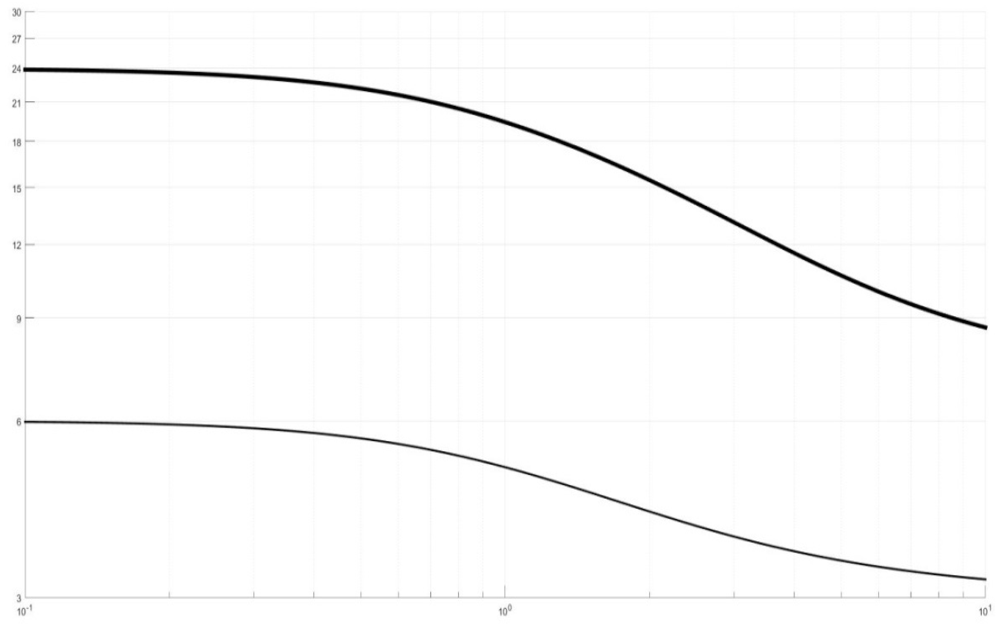
Figure 3 shows the behavior of the upper and lower bounds, indicated in Equation (29), of the kurtosis of the GCT expansions as n varies from 0.1 to 10 (see Figure 1 for comparison).
We now move to a GCT expansion of PHS distributions shaped on skewness accompanied by leptokurtosis. The intended density is specified as follows:
where is the monic polynomial of degree h, orthogonal with respect to the density function , is the squared norm of the aforementioned polynomial, and β and α are shape parameters subject to being non-negative definite.
Here and are as in Equations (21) and (22) and and are given by:
As usual p(x) stands for p(x,n).
Equation (34) provides the intended GCT expansion of subject to being positive definite, which occurs whenever the polynomial factor in the right-hand side is positive definite itself.
First we shall prove a lemma needed for proving the theorem we are primarily interested in.
Lemma 2.
With β as in Equation (26) of Lemma 1, the quartic polynomial:
parametric in α and β, is positive definite if α satisfies:
where is the smallest positive number for which the determinant of the Sylvester matrix:
vanishes. Here, υ, e, K, and d are written for υ(n), e(n), K(n), and d(n) for the simplicity of notation.
Proof.
With β as in Lemma 1, the property of positive definiteness once established for is maintained as we move to provided is small enough. It follows, on the one hand, that as long as is small enough the quartic in Equation (37) has two pairs of complex conjugate roots, and on the other hand that increasing will eventually attain a critical value at which positive definiteness no longer holds since one pair (at least) of complex conjugate roots collapses into a real double root. This marks the passage from definiteness to indefiniteness. Once the quartic in Equation (37) has a real double root, the determinant of the Sylvester matrix in Equation (39) associated with the polynomial vanishes, as well as its derivative (see, e.g., [12]). The foregoing argument leads to bound by the smallest at which such vanishing occurs.
Using Lemma 2 we can prove the main theorem.
Theorem 6.
The GCT expansion of the form
where is the standardized PHS distribution in Equation (10), is the quartic polynomial of Lemma 2 and α and β satisfy Equations (26) and (38), respectively, provide a family of leptokurtic skewed distribution functions.
The kurtosis is given by Equation (29), according to Theorem 5.
The skewness varies linearly with α, that is:
within the range of values:
where is as defined in Lemma 2.
Proof.
The proof follows the same lines as in the previous theorem and the argument of Lemma 2.
5. Entropy vs. Kurtosis of GCT Expansions
This section aims at shedding light on the behaviour of the entropy of the GCT expansion of Equation (17) as the extra-kurtosis parameter β runs from 0 to the upper bound specified in Equation (30).
To this end, we have to examine the integral:
where is as specified in Equation (17). In order to establish if the entropy decreases, as expected, as the extra-kurtosis parameter β moves upwards, we can look at the signature of its derivative with respect to β.
Simple computations show that:
First note that:
by the properties of orthogonal polynomials:
as the first and third factors under the integral sign turn out to be either both positive or both negative quantities.
Then, we need only look at the first term in the right-hand side of Equation (44) and examine the (sign of) the integral:
whose non-negativeness would provide a sufficient condition for the negativeness of the whole derivative of Equation (44), in light of Equations (45) and (46).
Some computations prove the intended result in the Laplace and Gaussian cases, namely:
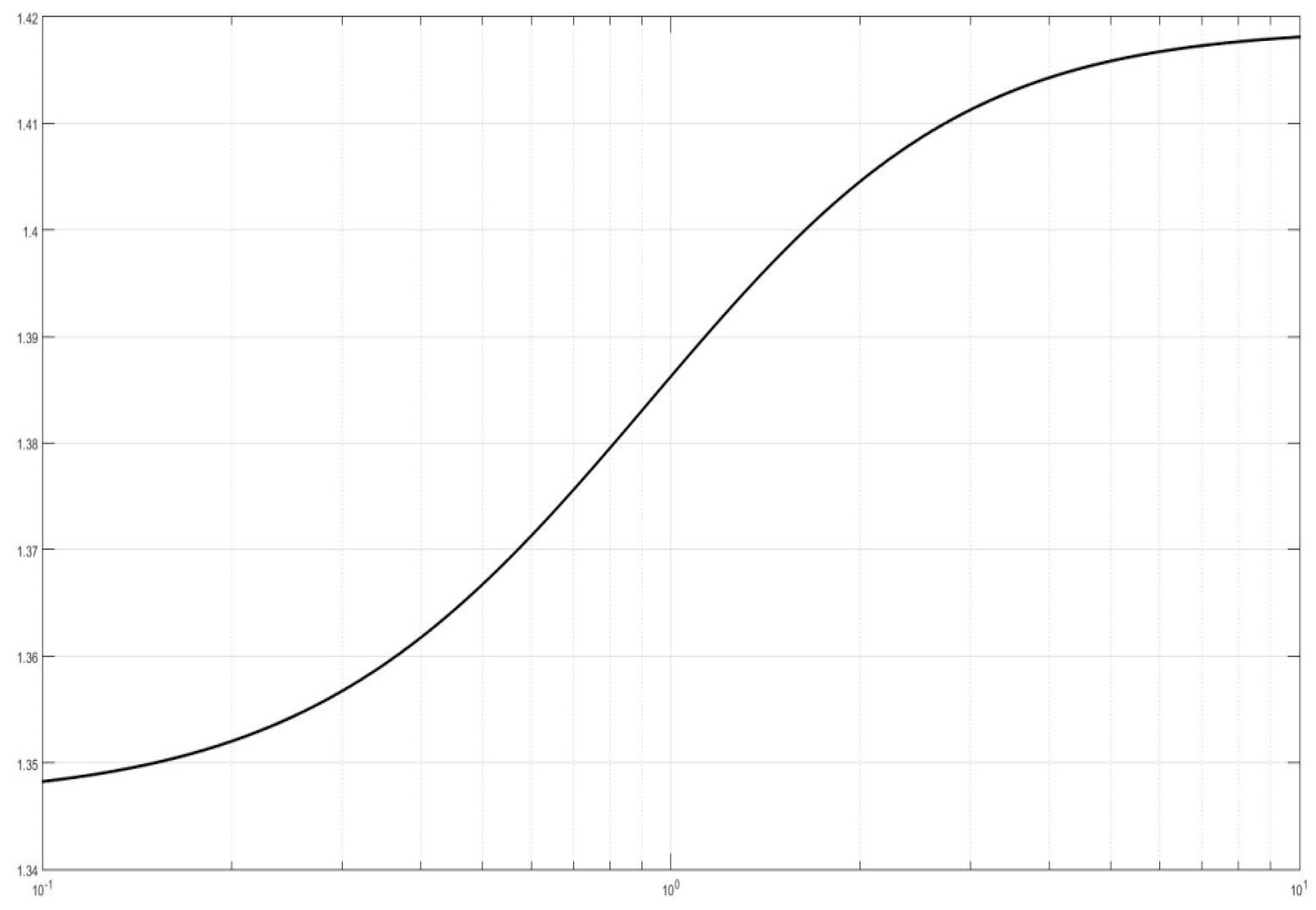
As for the behaviour of as n runs from 0 to ∞, a closed-form representation of the right-hand side of Equation (47) in terms of moment can be obtained by following an argument similar to that used in the proof of Theorem 4. However, analytic elegance aside, the closed-form so obtained would not prove of much interest. Thus, the behaviour of is given a graphic representation as shown in the chart here below.
Examining Figure 4 and given Equations (45) and (46), we realize that is a decreasing function of β: the entropy of GCT expansions drops as the excess-kurtosis grows.
The result provides further evidence of the (inverse) relation between entropy and kurtosis formerly recognized in Section 3.
6. GCT Expansions vs. Kurtosis: The Other Way Round
Figure 3 in Section 4 shows the feasibility region in the (K, n) plane, bounded by K and , where the GCT expansions of Equation (27) are definite positive.
Looking at the potential applications of the range of GCT distributions, the possibility of tracing a path across the aforesaid region is worth considering. This would entail joining the upper bound on the left (as n → 0) to the lower bound on the right (as n → ∞), which puts the level of kurtosis to be matched upon an empirical evidence argument, or a similar one, in a one-to-one correspondence with the parameter n identifying the PHS density and the intended GCT expansion, in turn.
From inspection of the aforesaid figure, the path across the positive-definitiveness region can be conceived as a reversed sigmoid curve, with inflection point at n = 2, in coordinates. The choice of the hyperbolic tangent as sigmoid function can be justified for analytic convenience by a heuristic argument. This leads to specifying the intended curve across the feasibility set as follows:
where:
Solving Equation (50) with respect to , as a function of n, yields:
as simple computations shows. In Figure 5 the graph of is superimposed on those of the boundary curves and K (see Figure 3 of Section 4).
Solving Equation (50) with respect to n as a function of gives:
This formula clears the way to bridging the potential of GCT expansions to model observed data under possibly severe condition of kurtosis, and the urge from of an empirical argument if this is the case.
In fact, in order to find the properly shaped distribution for a known or an estimated value of kurtosis, Equation (54) allows to establish the design parameter of the parent PHS density of the target GCT expansion to be determined.
To sum up, given a value of the required value of n is provided by Equation (54), which leads to specifying the intended density as follows:
where:
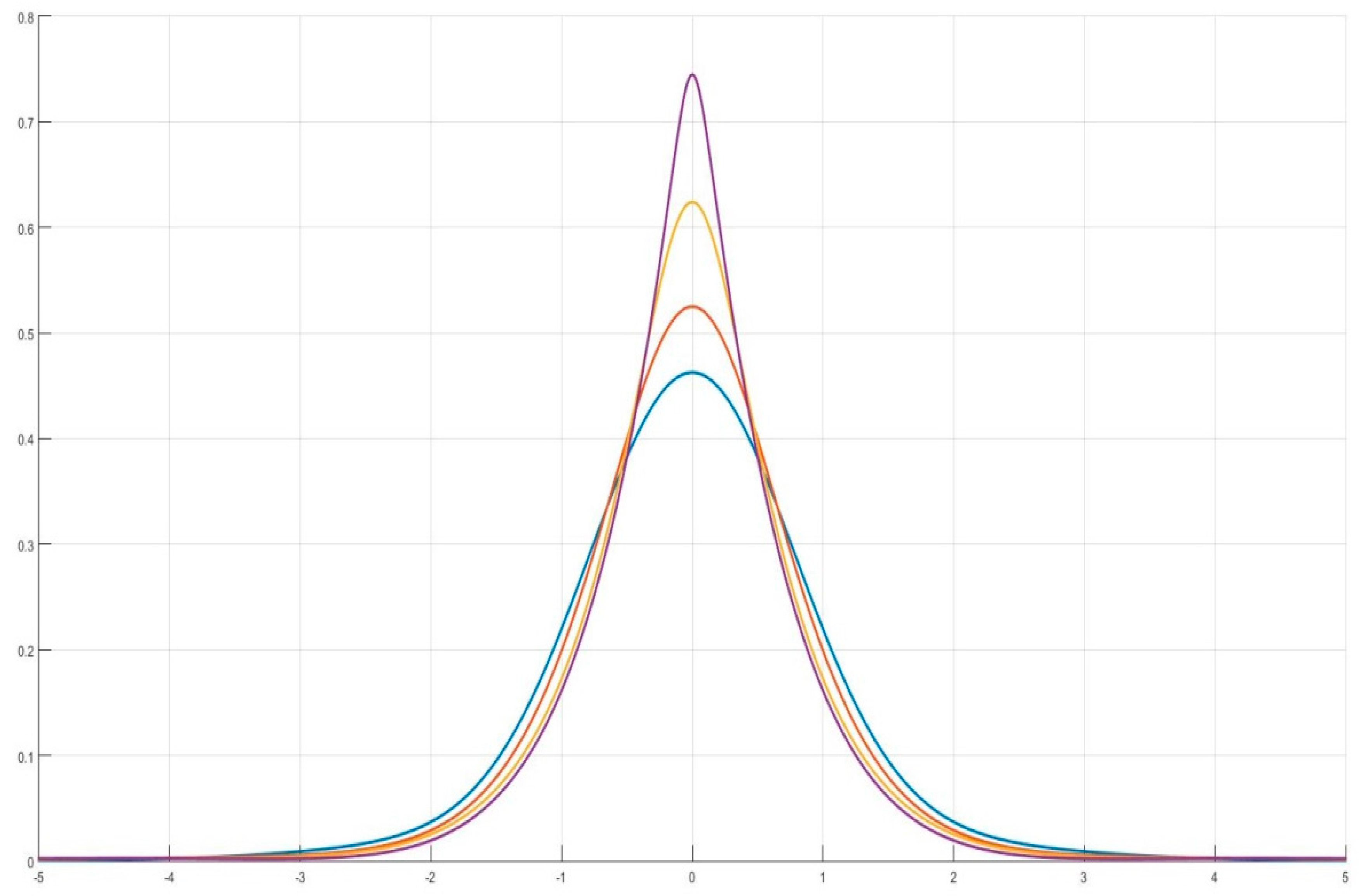
and the other symbols have the usual meaning. Figure 6 shows the graphs of f(x, ) for = 20, = 15, = 10 and = 5, in turn.
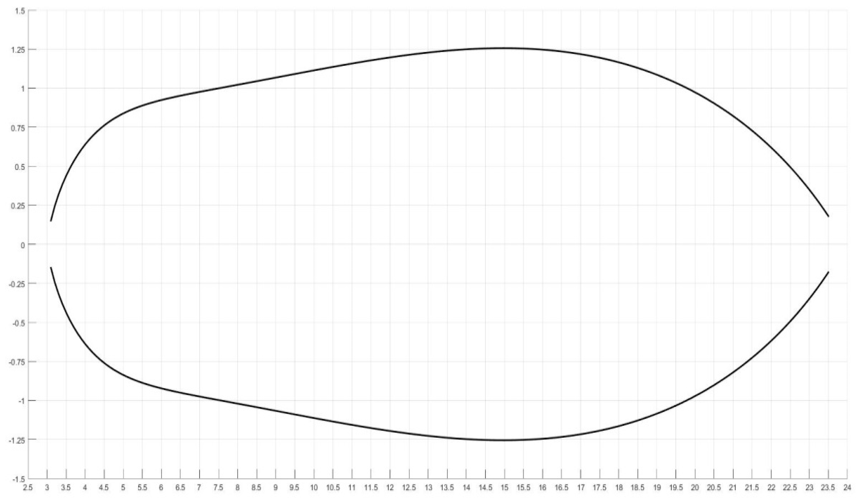
At this point, it is worth investigating to what extent a piece of information on skewness (α) can possibly be embodied into a GCT specification. To this end, we can follow an argument similar to that of Lemma 2 which leads to determining the feasibility region between the curves and , of the plane where the suitable GCT expansions are meaningful expressions. The locus of the , pairs for which positive definiteness of the intended GCT expressions is maintained, is depicted below in Figure 7.
Table 1 summarizes the previous results by showing the values of the design parameter n for the integer kurtosis level within the range , along with the maximum admissible skewness for meaningfulness of GCT expansions.
7. Concluding Remarks
The family of power-raised hyperbolic secant (PHS) distributions dealt with in this paper is characterized by a departure from normality as n increases. This is mirrored by both a growing kurtosis and a falling entropy. Cases of moderate leptokurtosis, which occur in several economic time series, are covered by the PHS family, but these distributions are unsuitable for these cases of severe excess kurtosis and asymmetry which are often found in financial data.
However, as the paper shows, this can be coped with Gram–Charlier-type (GCT) expansions based on orthogonal polynomials of f(x,n). This is, again, accompanied by a rise in the kurtosis along with a drop in entropy. The PHS family, and in particular its GCT expansions, provides an effective reference frame for modelling data whose departure from normality is evidenced by a thickness of the empirical distribution tails. Extensions to skewness effects clear the way to further applications, especially in financial econometrics.
Author Contributions
Both authors contributed equally to the paper. Both the authors have read and approved the final manuscript.
Conflicts of Interest
The authors declare no conflict of interest.
Appendix A
Proof of Theorem 1.
Given the integral representation of the beta function (see, e.g., [13], Vol. 1, p. 11):
evaluated at t = 0, and the functional relation:
it follows that:
Whence:
which qualifies as a density function.
The moment generating function:
ensues from (A1).
The cumulant generating function:
where is written for (n − 1)ln2 − lnb, follows accordingly.
The cumulants, as well as the moments of odd order, being zero, the cumulants of even order, , are obtained as follows:
which leads to a closed-form representation in terms of the polygamma functions of appropriate order, i.e.,:
Setting in Equation (A9) equal to 1 yields:
Now, replacing b with the above b(n) into Equation (3) leads to the standardized PHS:
where is written for .
Proof of Theorem 2.
The kurtosis is defined as:
Given Equations (A9), and working out Equation (A10), yields:
Now, inserting Equations (A9) and (A14) into Equation (A13) gives Equation (7).
The proofs of (i)–(ii) rest on the asymptotic representations of polygamma functions.
The representation of the trigamma function as z tends to infinite, can be obtained from the asymptotic expansion (see [15], Formula 6.4.12):
whose dominant term, as z , is . This proves that:
The representation of the pentagamma function as z tends to infinite, can be obtained from the asymptotic expansion (see [15], Formula 6.4.14):
whose dominant term, as z , is . Hence, the asymptotic representation:
holds.
From Equations (A16) and (A18), by setting z = , the following result:
is easily established.
This proves that the kurtosis tends to 3 as n .
Further, the asymptotic representation of the trigamma function as z tends to zero can be obtained from the expansion (see [16], Formula 5.15.1):
whose dominant term, as z → 0, is . This entails:
The representation of the pentagamma function as z tends to zero, can be obtained from the expansion (see [15], Formula 6.4.10):
whose dominant term, as z , is . Hence, the asymptotic representation:
holds.
From Equations (A21) and (A23), by setting , the following result:
is easily established.
This proves that the kurtosis index tends to 6 as n → 0.
Proof of Theorem 3.
The proofs of (i) and (ii) are based on the asymptotic representations (see, e.g., [17,18]) of the parameters a and b in formulas (2.2) and (A11), as n tends to infinity and to zero, in turn.
In light of Equation (A11), the asymptotic representation of b depends on that of the trigamma function. The asymptotic behavior of this latter as z tends to infinity, can be obtained from Equation (A15). Hence, the following holds as z tends to infinity:
whereas, in light of Equation (A21), the following proves true as z tends to zero:
According to Equation (2), and given Equation (A11), the asymptotic representations of a turns out to depend on both the trigamma and beta functions. As far as the latter is concerned, the asymptotic representation of beta as z tends to infinity is:
This can be established due to the functional relation ( see, e.g., [19], p. 950):
and making use of the asymptotic expansion (see [16], Formula 5.11.12):
The asymptotic representation of the beta function as z tends to zero can be obtained from the series expansion (see [19], Formula 8.382, 3):
whose dominant term, as z → 0, is . Hence:
Now, in light of (A25) and (A27), the following result:
is easily established.
Likewise, it follows from Equations (A26) and (A31) that:
These results pave the way to determining the asymptotic representation of the family of Equation (10) as n tends to infinite and zero, in turn.
To this end, it is helpful to rewrite Equation (A12) as follows:
where a and b are specified as in Equations (2) and (A11).
From the power series expansion:
along with Equations (A25) and (A32), the following asymptotic representation, as n tends to infinite:
is easily established.
Taking the limit of Equation (A36) as n approaches infinity yields:
as indicated in Equation (12).
Noting that , and taking the logarithm while given Equations (A26) and (A33), the following asymptotic representations hold:
as n tends to zero.
Taking the limit of Equation (A39) as n approaches zero yields:
as put forward in Equation (11).
Proof of Theorem 4.
According to (A3) the following holds:
This in turn, given the differentiation formula:
establishes that:
Now, consider the entropy of as specified in Equation (3), that is:
where for convenience use has been made of the change of variable .
By means of Equations (A42) and (A43), the entropy of Equation (A44) can be worked out as follows:
whence Equation (16) follows by simply taking b as indicated in Equation (A11).
References
- Benes, V.; Stepán, J. (Eds.) Distributions with Given Marginals and Moment Problems; Springer: New York, NY, USA, 1997. [Google Scholar]
- Fischer, M.J. Generalized Hyperbolic Secant Distribution; Springer: New York, NY, USA, 2014. [Google Scholar]
- Fischer, L.J.; Vaughan, D. The Beta-hyperbolic secant distribution. Aust. J. Stat. 2010, 3, 245–258. [Google Scholar]
- Vaughan, D.C. The generalized secant hyperbolic distributions and its properties. Commun. Stat. Theory Methods 2002, 31, 219–238. [Google Scholar] [CrossRef]
- Kendall, M.; Stuart, A. The Advanced Theory of Statistics; Distribution Theory; Griffin: London, UK, 1977; Volume 1. [Google Scholar]
- Zoia, M.G. Tailoring the Gaussian law for excess kurtosis and skewness by Hermite polynomials. Commun. Stat. Theory Methods 2010, 39, 52–64. [Google Scholar] [CrossRef]
- Bagnato, L.; Potì, V.; Zoia, M.G. The role of orthogonal polynomials in adjusting hyperbolic secant and logistic distributions to analyse financial asset returns. Stat. Pap. 2015, 56, 1205–1234. [Google Scholar] [CrossRef]
- Rényi, A. Probability Theory; North-Holland: Amsterdam, The Netherlands, 1970. [Google Scholar]
- Johnson, N.L.; Kotz, S.; Balakrisnam, N. Continuous Univariate Distributions, 2nd ed.; Wiley: New York, NY, USA, 1995; Volume 1. [Google Scholar]
- Chihara, T.S. An Introduction to Orthogonal Polynomials; Gordon & Breach: New York, NY, USA, 1978. [Google Scholar]
- Szegö, G. Orthogonal Polynomials; American Mathematical Society: Providence, RI, USA, 1939. [Google Scholar]
- Gelfand, I.M.; Kapranov, M.M.; Zelevinsky, A.V. Discriminants, Resultants and Multidimensional Determinats; Birkhauser: Boston, MA, USA, 1994. [Google Scholar]
- Erdélyi, A.; Magnus, W.; Oberhettinger, F.; Tricomi, F.G. Higher Transcendental Functions; Mc. Graw Hill: New York, NY, USA, 1953. [Google Scholar]
- Lloyd, E. Probability. In Handbook of Applicable Mathematics; Ledermann, W., Ed.; Wiley: New York, NY, USA, 1980; Volume 2. [Google Scholar]
- Davis, P.J. Gamma Function and Related Functions. In Handbook of Mathematical Functions; Abramovitz, M., Stegun, I.A., Eds.; Dover: New York, NY, USA, 1965. [Google Scholar]
- Askey, R.A.; Roy, R. Gamma Function. In NIST Handbook of Mathematical Functions; NIST and Cambridge University Press: Cambridge, UK, 2009. [Google Scholar]
- Copson, E.T. Asymptotic Expansions; Cambridge University Press: Cambridge, UK, 1965. [Google Scholar]
- Erdélyi, A. Asymptotic Expansions; Dover: New York, NY, USA, 1965. [Google Scholar]
- Gradshteyn, I.S.; Ryzhik, I.M. Table of Integrals, Series and Product; Academic Press: London, UK, 1980. [Google Scholar]
Figure 1.
Graph of the kurtosis of PHS distributions as a function of n (log scale).

Figure 2.
Graph of the entropy of PHS distributions as a function of n (log scale).

Figure 3.
Graphs of the upper bound (bold line) and lower bound of the kurtosis of the GCT expansions as n varies from 0.1 to 10 (log-log scale).
Figure 3.
Graphs of the upper bound (bold line) and lower bound of the kurtosis of the GCT expansions as n varies from 0.1 to 10 (log-log scale).

Figure 4.
Graph of the function as n varies from 0.1 to 10 (log scale).

Figure 5.
From top to bottom: graphs of , (bold line) and K as n varies from 0.1 to 10 (log-log scale).
Figure 5.
From top to bottom: graphs of , (bold line) and K as n varies from 0.1 to 10 (log-log scale).
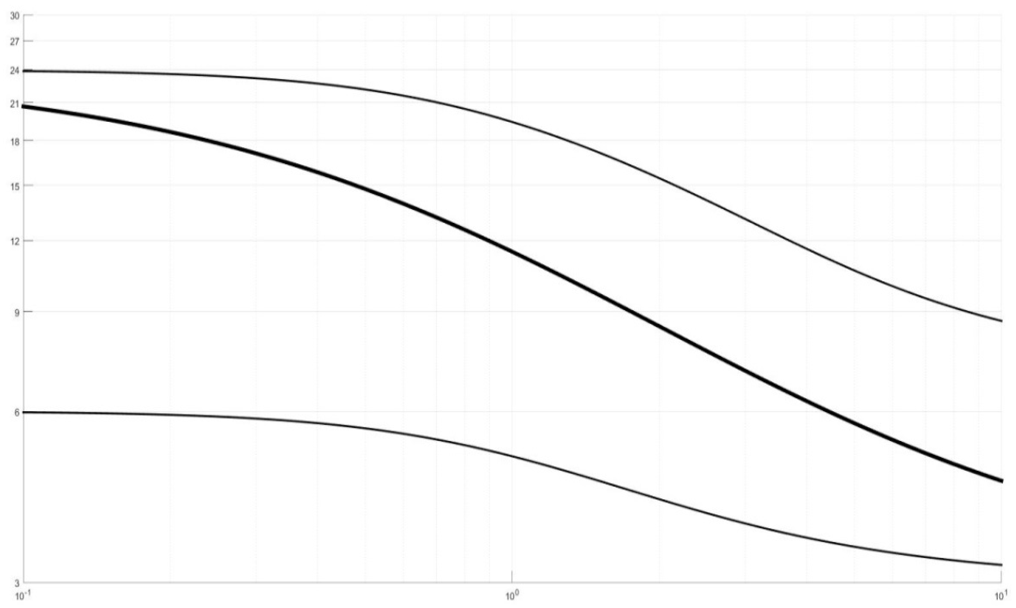
Figure 6.
From top to bottom: graphs of GCT-PHS densities for = 20, 15, 10, 5.

Figure 7.
Chart of the , plane showing the region of positive definiteness of GCT.


Table 1.
Values of n and bounds of skewness for = 4–23.
| n | ||
|---|---|---|
| 4 | 16.407 | 0.639183439 |
| 5 | 7.267 | 0.837626059 |
| 6 | 4.4349 | 0.923283996 |
| 7 | 3.0721 | 0.975361836 |
| 8 | 2.2741 | 1.021018199 |
| 9 | 1.751 | 1.066996287 |
| 10 | 1.3822 | 1.113102509 |
| 11 | 1.1084 | 1.157085560 |
| 12 | 0.8974 | 1.196177300 |
| 13 | 0.7301 | 1.227518579 |
| 14 | 0.5944 | 1.248241505 |
| 15 | 0.4824 | 1.255447821 |
| 16 | 0.3886 | 1.246145088 |
| 17 | 0.3092 | 1.217143588 |
| 18 | 0.2415 | 1.164894037 |
| 19 | 0.1833 | 1.085226615 |
| 20 | 0.1331 | 0.972914475 |
| 21 | 0.0899 | 0.820895356 |
| 22 | 0.0529 | 0.618745392 |
| 23 | 0.0220 | 0.349248618 |
© 2017 by the authors. Licensee MDPI, Basel, Switzerland. This article is an open access article distributed under the terms and conditions of the Creative Commons Attribution (CC BY) license (http://creativecommons.org/licenses/by/4.0/).
Share and Cite
MDPI and ACS Style
Faliva, M.; Zoia, M.G. A Distribution Family Bridging the Gaussian and the Laplace Laws, Gram–Charlier Expansions, Kurtosis Behaviour, and Entropy Features. Entropy 2017, 19, 149. https://doi.org/10.3390/e19040149
AMA Style
Faliva M, Zoia MG. A Distribution Family Bridging the Gaussian and the Laplace Laws, Gram–Charlier Expansions, Kurtosis Behaviour, and Entropy Features. Entropy. 2017; 19(4):149. https://doi.org/10.3390/e19040149
Chicago/Turabian StyleFaliva, Mario, and Maria Grazia Zoia. 2017. "A Distribution Family Bridging the Gaussian and the Laplace Laws, Gram–Charlier Expansions, Kurtosis Behaviour, and Entropy Features" Entropy 19, no. 4: 149. https://doi.org/10.3390/e19040149
Note that from the first issue of 2016, this journal uses article numbers instead of page numbers. See further details here.