
Unsupervised Symbolization of Signal Time Series for Extraction of the Embedded Information


Department of Mechanical & Nuclear Engineering, Pennsylvania State University, University Park, PA 16802, USA
*
Author to whom correspondence should be addressed.
Entropy 2017, 19(4), 148; https://doi.org/10.3390/e19040148
Submission received: 20 January 2017
/
Revised: 17 March 2017
/
Accepted: 28 March 2017
/
Published: 31 March 2017
(This article belongs to the Special Issue Symbolic Entropy Analysis and Its Applications)
Abstract
:This paper formulates an unsupervised algorithm for symbolization of signal time series to capture the embedded dynamic behavior. The key idea is to convert time series of the digital signal into a string of (spatially discrete) symbols from which the embedded dynamic information can be extracted in an unsupervised manner (i.e., no requirement for labeling of time series). The main challenges here are: (1) definition of the symbol assignment for the time series; (2) identification of the partitioning segment locations in the signal space of time series; and (3) construction of probabilistic finite-state automata (PFSA) from the symbol strings that contain temporal patterns. The reported work addresses these challenges by maximizing the mutual information measures between symbol strings and PFSA states. The proposed symbolization method has been validated by numerical simulation as well as by experimentation in a laboratory environment. Performance of the proposed algorithm has been compared to that of two commonly used algorithms of time series partitioning.
1. Introduction
Symbolic time series analysis, as a data interpretation technique, has been studied in the open literature for over a century [1]. The concepts of symbolic dynamics-based analysis have been applied to many research topics such as: communication encoding in information theory by Shannon [2], information extraction in supervised data-mining by Lin et al. [3], symbolic time series analysis of experimental data by Daw et al. [4], anomaly detection and pattern recognition by Ray [5] and Mukherjee and Ray [6], and Markov decision processes in discrete dynamical systems by Puterman [7]. In such processes, changes in the statistical patterns of dynamic behavior may often occur over a slow time scale with respect to the fast time scale of process dynamics. from this perspective, the concept of two time scales is succinctly presented below.
Definition 1.
(Fast Scale) The fast scale is defined to be a time scale over which the statistical properties of the process dynamics are assumed to remain invariant, i.e., the process is assumed to have statistically stationary dynamics at the fast scale.
Definition 2.
(Slow Scale) The slow scale is defined to be a time scale over which the statistical properties of the process dynamics may gradually evolve, i.e., the process may exhibit statistically non-stationary dynamics at the slow scale.
In view of Definition 1, statistical variations in the internal dynamics of the process are assumed to be negligible at the fast scale. Thus, sensor time series data are acquired based on the assumption of statistical stationarity at the fast scale. In view of Definition 2, an observable non-stationary behavior could be associated with the gradual evolution of anomalies (i.e., deviations from the nominal behavior) in the process at the slow scale. In general, a long time span at the fast scale is a tiny (i.e., several orders of magnitude smaller) interval at the slow scale.
The major steps for information extraction from sensor signal outputs (e.g., time series) of a dynamical system are as follows:
- Coarse-graining of time series to convert the scalar or vector-valued data into symbol strings, where the symbols are drawn from a (finite) alphabet [8].
In this context, information loss is often a concern in symbolization of a continuous time series that is discretized into the corresponding symbol series. This issue has been addressed by Beim Graben [10] in the sense that symbolization can directly improve signal-to-noise ratio (SNR) in noise-contaminated signals. In addition, symbolization makes digital communication and numerical computation more efficient and effective as compared to similar operations with continuous-valued data. Discussions on advantages of working with symbolized data can be found for different applications (e.g., see [5,6,11,12]).
There are two main tasks in time series symbolization [4,13], namely, (i) definition of symbols, and (ii) construction of words (i.e., symbol blocks) that have relevance for information representation [5,6]. A commonly used approach is to partition the range of time-series data into a finite number of mutually exclusive and exhaustive segments. Each segment is associated with a unique symbol, to which all data points in that segment are mapped accordingly. The choice of the total number of symbols (i.e., alphabet size) may range from 2 to the number of distinct data points in the time series. In ideal (e.g., noise-free) data, more information is retained as the alphabet size is increased; however, the effects of any spurious disturbances (e.g., measurement noise) in the data could be detrimental if the alphabet size is arbitrarily increased [10]. After the symbols are defined, the next task is to determine the (finite-length) symbol blocks, also called words, which represent meaningful temporal patterns. This step is crucial for generating dynamical models from the symbol series that can be used for event prediction [14]. Construction of words is analogous to time-delay embedding in the phase space [15], where a combination of words may contain ”complete” dynamical information of the symbol series. The results, generated from word construction, can be represented as a context tree in a variable-order Markov model [16], where the symbols in a series with Markov property depend on the previous symbol blocks (i.e., words). Naturally, some words may not exist since they do not appear at all for a given symbol series, and some existing words may not have any significant contribution to the system dynamics. Therefore, instead of investigating all possible words with (or up to) a fixed length, it is desirable to explore the potentially meaningful words with adaptive and individual length increments to achieve variable embedding [14].
Several researchers (e.g., Sarkar et al. [13]) have shown that both alphabet size and partitioning map would influence preservation of the original information in the generated symbol series; therefore, the choice of both the number of symbols and partitioning locations are crucial for subsequent signal analysis. To appropriately choose partitioning locations in the time series generated by a dynamical system with unknown noise, several ad hoc methods have been reported in the literature. For example, Rajagopalan and Ray [9] investigated two partitioning schemes, namely, maximum entropy partitioning (MEP) (which is based on equal frequency of symbol occurrence) and uniform space partitioning (USP) (which is based on equal partitioning segment width) for one-dimensional data. Ahmed et al. [17] investigated a data discretization technique called frequency dynamic interval class (FDIC), which is based on the data statistical frequency measure and k-nearest neighbor (kNN) algorithm [18]. To obtain ”optimal” partitioning locations, Shannon entropy measure [2] has been used by researchers to maximize the dynamic information level in the symbol series. For example, Lehrman et al. [19] defined an entropy measure of information contents in the symbol series and maximized it by an optimization process based on the number of symbols and locations of partitions. Mörchen et al. [20] proposed an unsupervised discretization algorithm based on the Kullback–Leibler divergence [21] between the marginal and self-transition probability distribution of the symbol series. Other studies have been reported to address word construction with variable embedding. For example, Kennel and Mees [14], motivated by the minimum description length (MDL) principle [22] and context tree weighting (CTW) algorithm [23], constructed a compact and robust context-tree predictive model via a finite-state automaton with probabilistic emission probabilities. Mukherjee and Ray [6] proposed a state splitting (i.e., increment of word length) and merging (i.e., decrement of word length) algorithm by minimizing the conditional entropy measures between symbols and potential words in the symbolic series.
To the best of the authors’ knowledge, a majority of symbolic time series analysis approaches reported in literature treat symbol definition and word selection as two separate tasks. In contrast, the current paper proposes an algorithm that chooses the symbols and words simultaneously in an unsupervised way by maximizing their mutual information measures. In this procedure, a set of potential partitioning boundary locations is assumed as an initial condition; then, more segments are iteratively created in the existing partition to accommodate an additional symbol in the alphabet. For each potential partition location, the corresponding word set is obtained by maximizing the mutual information measure between the respective symbol and the word. The potential partitioning boundary location with the highest mutual information is chosen and added to the existing partition. Based on a stopping rule, new symbols are added until the mutual information stops increasing.
The proposed method has been validated by numerical simulation as well as by experimentation in a laboratory environment, and its performance has been compared with those of several commonly used methods of signal discretization. In the context of dynamic data-driven application systems [24], major contributions of the work reported in this paper are delineated below:
- Unsupervised symbolization of time series: Simultaneous selection of symbols and words based on information-theoretic measures.
- Word selection for a given symbolic series: Adaptive variable embedding based on the mutual information between symbols and potential words.
- Determination of symbol alphabet size: Prevention of excessive symbolization for information extraction.
- Validation on both simulation and experimental data: Demonstration of performance robustness with presence of added zero-mean Gaussian noise and background noise of varying environment.
The rest of the paper is organized as follows. Section 2 presents the underlying mathematical concepts and principles applied in this paper. Section 3 formulates the time series symbolization problem in the framework of information-theoretic Markov modeling. Section 4 elaborates the technical approach of unsupervised time series symbolization adopted in this paper. Section 5 validates the proposed concepts on a number of artificial and realistic experimental data sets by comparison with two commonly used methods of time series partitioning. Section 6 concludes the paper along with recommendations for future research.
2. Mathematical Preliminaries
This section presents the basic concepts and principles in finite automata and information theory, which are applied in this paper for time series symbolization. The details of proofs can be found in Chapters 1, 2 and 6 of Lind and Marcus [8] as well as in [25,26].
2.1. Probabilistic Deterministic Finite Automata
Definition 3 (Deterministic finite automaton).
A Deterministic finite automaton (DFSA) [27] is a 5-tuple where:
- 1.
- Σ is a non-empty finite set, called the symbol alphabet;
- 2.
- is a non-empty finite set, called the set of states;
- 3.
- is the state transition map;
- 4.
- is a set of initial states ();
- 5.
- is a set of final states ().
An automaton is called trim [26] if any state is accessible from and can access .
Since this paper deals with finite trim automata, where all states belong to both and , (i.e., and ), the deterministic finite automaton is denoted as a 3-tuple in the sequel.
Definition 4 (PFSA [28]).
A probabilistic finite-state automaton (PFSA) is constructed on the algebraic structure of deterministic finite-state automata (DFSA) as a pair , i.e., the PFSA is a 4-tuple , where:
- 1.
- Σ is a non-empty finite set, called the symbol alphabet, with cardinality ;
- 2.
- is a non-empty finite set, called the set of states, with cardinality ;
- 3.
- is the state transition map;
- 4.
- is the symbol generation matrix (also called probability morph matrix) that satisfies the condition , and is the probability of emission of the symbol when the state is observed.
Remark 1.
The above structure of PFSA allows a rich library of possible words with a small alphabet. For example, if the alphabet and the maximum length of each word is 3, then one may have a mixture of words from length 1 to 3 such as, , and 111. More elaborate examples are given by Mukherjee and Ray [6].
A special class of PFSA is now introduced, which is called D-Markov machine. This class of models has a simple algebraic structure and is computationally efficient for construction and implementation.
Definition 5 (-Markov Machine [5,6]).
Let be a discrete symbol string that is assumed to be a statistically stationary stochastic process. The probability of occurrence of a new symbol depends only on the most recent D consecutive symbols, where D is a positive integer, i.e.,
where D is called the depth of the D-Markov machine. Then, a D-Markov machine (presented as a PFSA in which each state is represented by a finite history of D symbols) is defined as a 4-tuple such that:
- 1.
- is the state set corresponding to a symbol string , where is the (finite) cardinality of the state set.
- 2.
- is the alphabet set of symbol string , where is the (finite) cardinality of the alphabet Σ of symbols.
- 3.
- is the state transition mapping. It is noted that the PFSA structure is built on and thus, the transition map explains the same symbol string;
- 4.
- is the morph matrix of size ; the -th element of Π denotes the probability of finding the symbol at next time step while making a transition from the state .
Thus, the symbol string is compressed as a PFSA by approximating the states by words of finite length from the symbol sequence. The PFSA induces a Markov chain of finite order where the parameters of the Markov chain, i.e., the stochastic matrix is estimated from data by following a maximum a priori probability (MAP) approach under the assumptions of sufficiently long data [6]. Once the parameters are estimated, they are used as a temporal representation for the underlying data, which can be used for different machine learning applications (e.g., pattern matching and clustering) [18].
2.2. Information Theory
Definition 6 (Shannon Entropy [29]).
The Shannon entropy H of a discrete random variable X with possible values and probability mass function is defined as:
The Shannon entropy of X describes the uncertainty or unpredictability of the information content in X. The base of the logarithm used in this paper for entropy calculation is Euler’s number (i.e., the number e).
Definition 7 (Conditional Entropy [29]).
The conditional entropy of the random variable Y given a random variable X is defined as:
where is the conditional probability of given that is observed.
Definition 8 (Mutual Information [29]).
Formally, the mutual information of two discrete random variables X and Y is defined as:
The mutual information is a measure of the mutual dependence between two random variables and it can be equivalently expressed as:
2.3. Distance Measurement for Symbol Sequences
Definition 9 (Hamming Distance).
Let and be two symbol strings of the same (finite) length L. Then, the (scalar) Hamming distance between these two symbol strings is defined as:
where
Definition 10 (Average Linkage).
Let and be two clusters, each of which contains at least one symbol string and all symbol strings therein have the same length. Let be the number of symbol strings in cluster , and let and be the i-th and j-th symbol strings, respectively, in the cluster . Then the average linkage , which uses the average distance between all pairs of objects in any two clusters, is defined as:
3. Problem Statement
This section formulates the problem of time series symbolization in the framework of information-theoretic Markov modeling. There are three basic problems of interest that must be solved to extract the embedded temporal behavior in the (possibly processed) time series signal under consideration. These three problems are delineated below:
- Problem#1: Determination of the alphabet size , which is the number of symbols in the alphabet , for representation of the time series as a string of symbols.
- Problem#2: Identification of the partitioning boundary locations, , which quantizes the signal space into a finite number of mutually exclusive and exhaustive regions. Each region is associated with a unique symbol, to which the time series signal in that region is mapped.
- Problem#3: Identification of the state set , which consists of meaningful (i.e., relevant) symbol patterns that could reduce the uncertainty of the temporal transition in the symbol sequence [10].
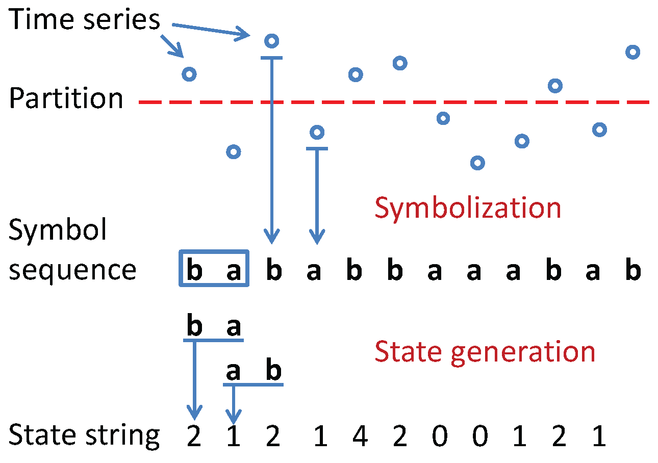
Problem and Problem together define the symbol assignment in a time series. The procedure of time series symbolization is elucidated by an example in Figure 1. While systematic suboptimal procedures for alphabet size selection has been reported in literature (e.g., [13]), the alphabet size in the example of Figure 1 is selected ad-hoc and is application-dependent. This practice is often followed because the computation complexity of the symbolic time series is approximately proportional to the alphabet size, while the information gain for an increase in alphabet size is not. In this context, the information gain is measured by the Shannon entropy excess, which is defined as a measure of the increment in maximum Shannon entropy value of n symbols from symbols.
Definition 11 (Shannon Entropy Excess [30]).
The Shannon entropy excess for n symbols is the increment in maximum uncertainty as the new symbol is added to the existing n symbols in the alphabet.
where is defined by the uniform distribution of the symbols to achieve the maximum uncertainty, and .
Figure 2 depicts the profiles of maximum Shannon entropy and entropy excess as functions of the alphabet size . As is increased, the Shannon entropy excess is decreased. So, it is logical to make a trade-off between the computational complexity and the information loss when determining the alphabet size during time series symbolization [6].
Once the alphabet size is determined, the next step is identification of partitioning boundary locations. The objective here is to obtain a symbol sequence that will retain temporal transition behavior embedded in the time series signal. As mentioned earlier in Section 1, a generating partition would be desirable from the perspectives of information retention; however, the necessary conditions for existence of a generating partition include: a noise-free and infinitely long time series, which cannot be guranteed in real-life situations. It is noted that there exist a few ad-hoc unsupervised algorithms that can generate partitioning boundary locations for a given (one-dimensional) finite length time series in special cases (e.g., (one-dimensional) logistic map).
Rajagopalan et al. [9] have reported a maximum entropy partitioning (MEP) algorithm (also known as equal frequency partition), where the key idea is to uniformly distribute the occurrence probability of each symbol in the generated symbol sequence such that the information-rich regions of the time series are partitioned finer and those with sparse information are partitioned coarser. In general, Shannon entropy of a (finite) symbol sequence is approximately expressed as:
where is the probability of occurrence of the symbol . Algorithm 1 explains the procedure of maximum entropy partitioning (MEP), which has been used in this paper; the entropy of the symbol sequence is maximized because .
The next task is to discover the temporal patterns from the generated symbol sequence, where the PFSA states are identified by selecting relevant strings of symbols in a temporal order. There are two basic criteria to evaluate the significance of a possible symbol block with a finite length D:
- Crterion#1: The frequency of the symbol block occurring in the symbol sequence.
- Crterion#2: Influence of the symbol block on the next observed symbol in temporal order.
If a certain symbol block appears frequently in the symbol sequence while the distribution of the symbol observed next to it is statistically relevant (e.g., not randomly occurring), then the symbol block is qualified to be a state. It is noted that the relevant symbol blocks for a given symbol sequence may not be of equal length. Mukherjee and Ray [6] proposed a state splitting and merging algorithm to identify states with different lengths by making use of an information-theoretic measure between states and symbols in terms of the conditional entropy.
| Algorithm 1 Maximum Entropy Partitioning |
| Require: Finite-length time series |
| and alphabet size . |
| Ensure: Partition position vector |
| 1: Sort the time series in the ascending order; |
| 2: Let K=length(), which is the length of the time series; |
| 3: Assign = , i.e., the minimum element of |
| 4: for i=2 to do |
| 5: = |
| 6: end for |
| 7: Assign = , i.e., the maximum element of |
Definition 12 (Conditional entropy on a single state).
The conditional entropy of the symbol alphabet Σ conditioned on a single state is defined as:
where is the conditional probability of a symbol given that a state (i.e., a relevant symbol block) q has been observed.
Definition 13 (Conditional entropy on a state set).
The conditional entropy of the symbol alphabet Σ on a state set is defined as:
Mukherjee and Ray [6] have claimed that lower is the conditional entropy, more predictable is the next observed symbol conditioned on the current state. As conditional entropy approaches 0, the next observed symbol tends to be deterministic.
To the best of authors’ knowledge, most publications in the open literature have treated these questions separately as examples mentioned above. In the next section, an unsupervised algorithm is presented, which addresses these basic issues in time series symbolization within a unified information-theoretic framework.
4. Technical Approach
This section proposes an unsupervised algorithm of time series symbolization (i.e., with no requirement for labeling of time series), based on information-theoretic Markov modeling of time series. The symbolization process identifies a partitioning vector that maximizes the mutual information between the symbols in and the states in as:
In Equation (12), the mutual information consists of two terms, where the first term is the entropy of the symbols in and the second term is the conditional entropy of the symbols in given the states in . It is noted that the symbol alphabet is completely characterized by its cardinality (i.e., the number of symbols in ) and vector of partitioning locations that form boundaries of the partitioning segments in the alphabet construction. Therefore, in Equation (12) is equivalently expressed as . Referring to the three problems in Section 3, the symbolization task is formulated as the following optimization problem:
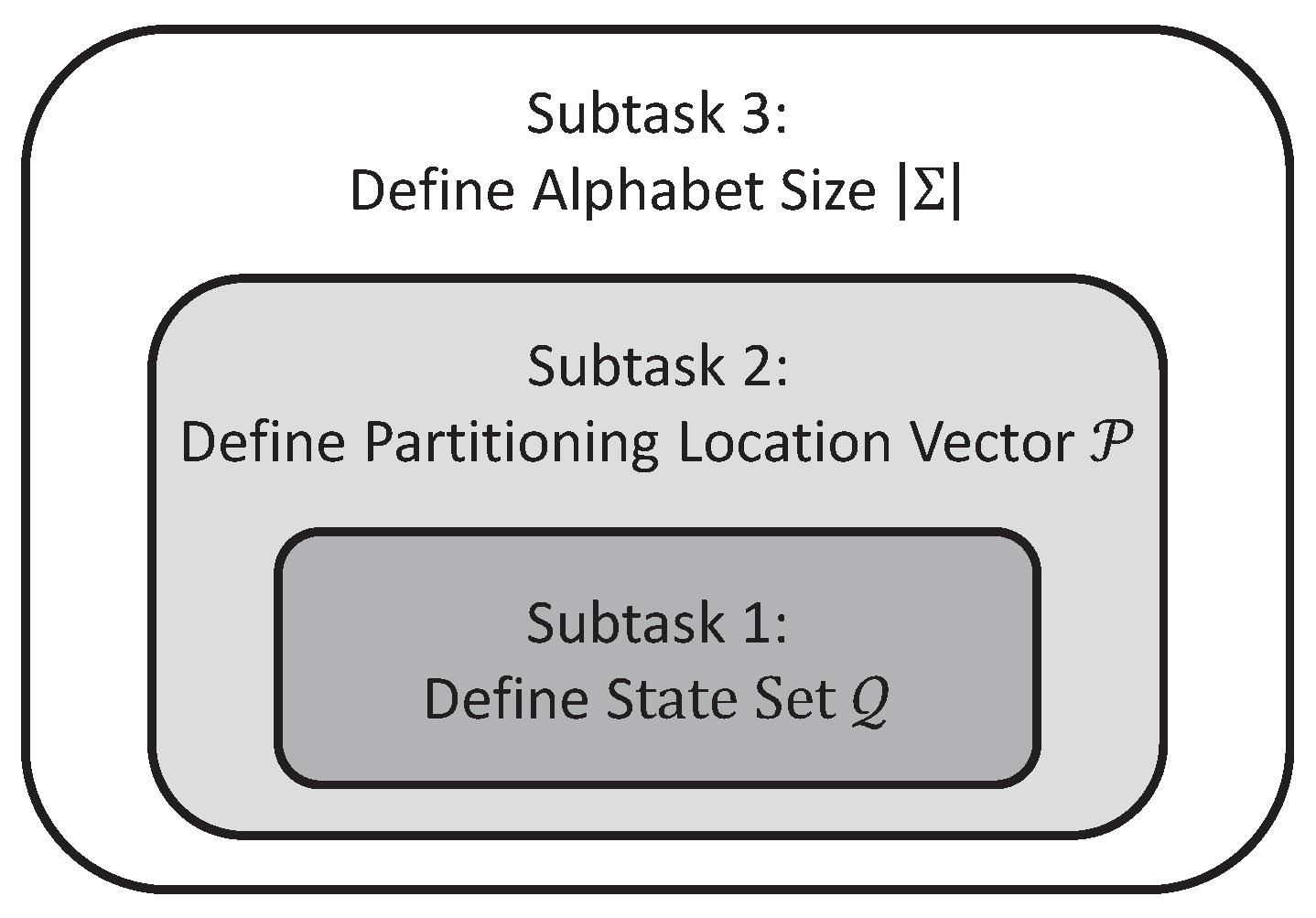
In general, the above optimization problem is non-convex and NP-hard. Therefore, a greedy search strategy has been adopted in this paper, which consists of the following three subtasks:
- Subtask 1: Identification of the state set that maximizes the mutual information via variable Markov Modeling for any given alphabet size and partitioning location vector .
- Subtask 2: Identification of the partitioning location vector among a pre-defined candidate set, which maximizes the mutual information for any given alphabet size , while the state set is obtained from Subtask 1 for each individual candidate.
- Subtask 3: Identification of the alphabet size , which maximizes the mutual information , while the state set and the partitioning location vector are obtained from Subtask 1 and Subtask 2, respectively, for each choice of alphabet size .
In Subtask 1, the entropy of symbol emission probability for each state is computed as the conditional entropy between symbols and states. In Subtask 2, the partitioning locations are chosen from a pre-defined candidate set, based on the maximum entropy partitioning (MEP) of the given time series. In Subtask 3, the alphabet size is recursively increased until the resulting increment of computed mutual information is not significant based on a predefined threshold. A quantitative demonstration of real-time execution of the proposed method is a topic of future research as stated in Section 6.
Remark 2.
Although the above three-stage method does not exactly represent the optimization problem as stated in Equation (13), these three modifications (with appropriately chosen thresholds) are expected to reduce the computational cost in the proposed method at the expense of (moderately) increased optimality loss. Potentially, the proposed iterative process is guaranteed to reach truly “global” optima, but instead may settle on “local” optima in some cases. This is a potential cost required to achieve results from the 3D search within a reasonable length of time. The rationale for this approximation is that the computational cost of greedy search in a 3-D space could be too large to be acceptable for real-time implementation.
Figure 3 depicts the relationship and dependence among the three subtasks 1, 2 and 3, where mutual information is maximized at different stages of the the proposed greedy search algorithm. Subtask 1 identifies the state set (see Algorithm 2) for a given alphabet , i.e., specified alphabet size and partitioning location vector . Then, Subtask 2 identifies the partitioning location vector (see Algorithm 3) with the state set identified in Subtask 1 and a specified alphabet size . Finally, Subtask 3 is solved for different choices of alphabet size with the identified state set and partitioning location vector . Further details of these subtasks follow.
| Algorithm 2 State Splitting for Variable-Depth D-Markov Machine |
| Require: Symbol sequences |
| threshold for state splitting and |
| Ensure: State set |
| 1: Initialize: Create a 1-Markov machine |
| 2: repeat |
| 3: |
| 4: for i=1 to do |
| 5: if and then |
| 6: |
| 7: end if |
| 8: end for |
| 9: until |
| Algorithm 3 Partitioning by Sequential Selection Based on an Information-Theoretic Measure |
| Require: Time series , Alphabet size , and number, m, of candidate partitioning locations. |
| Ensure: Partitioning location vector and the maximum mutual information for alphabet size . |
| 1: Create the set of candidate partitioning locations via MEP in Algorithm 1. |
| 2: Assign the partitioning location vector and . |
| 3: for n=2 to do |
4: Obtain locally optimal partitioning
|
| 5: The specific partitioning location , corresponding to the the maximum mutual information , is removed from C and is included in the set of selected partitioning locations to construct the locally optimal . |
| 6: end for |
4.1. Subtask 1: Determine the State Set
For a given symbol sequence over the alphabet (i.e., alphabet size and partitioning location vector ), the locally optimal state set is obtained by maximizing the mutual information. Since the symbol entropy is independent of the choice of states, which is carried out by minimizing the conditional entropy :
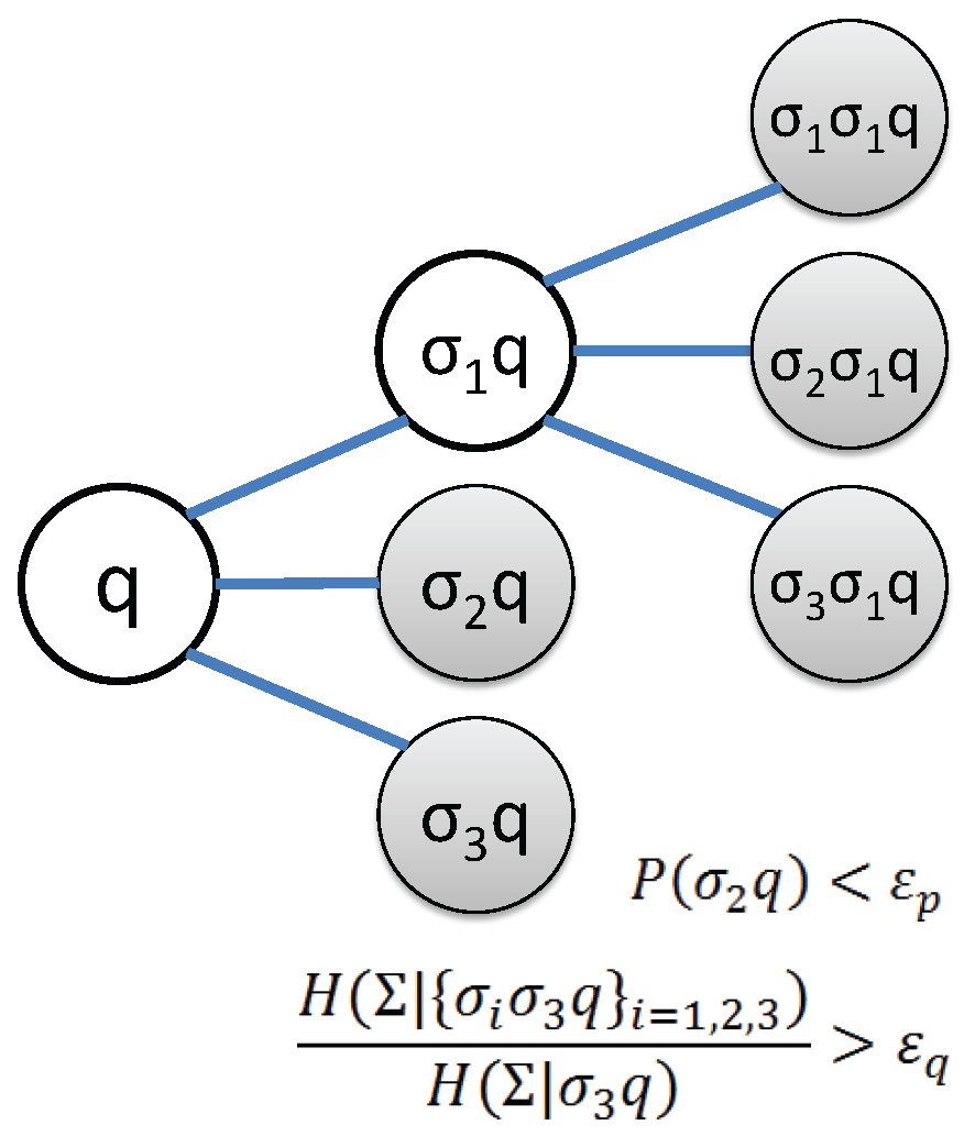
Identification of the state set starts off with the simplest set of states (i.e., ) and subsequently splitting the current state results in the largest decrease of the conditional entropy. The process of splitting a state is executed by replacing the symbol block for q by its branches given by the set . Then, the maximum reduction of the conditional entropy of the PFSA is the governing criterion for selecting the state to split. Figure 4 depicts an example to clarify the concept, based on the following two criteria in state splitting:
- Threshold for occurrence probability , indicating whether a state has relevant statistical information or not.
- Threshold for conditional entropy reduction that determines whether states of longer memory is necessary or not.
As a result, not all the states are split and a variable-structure PFSA is created. State splitting for inferring the PFSA is delineated as Algorithm 2. The parameters of the Markov model are estimated using maximum a posteriori (MAP) rule with uniform prior. Let denote the number of times that a symbol is generated in when the state as the symbol string is observed in the PFSA . The maximum a posteriori probability (MAP) estimate of the emission probability of the symbols conditioned on is estimated by frequency counting [6] as follows.
The rationale for initializing each element of the count matrix N to 1 in Equation (15) is that if no event is generated at a state , then there should be no preference to any particular symbol and it is logical to have , i.e., the uniform distribution of event generation at the state q. The above procedure guarantees that the PFSA, constructed from a (finite-length) symbol string, must have an (elementwise) strictly positive morph map in Definition 4.
4.2. Subtask 2: Identification of Partitioning Locations
The partitioning location vector is identified as a sequential selection process. First, a collection of candidate partitioning locations ’s is obtained as by maximum entropy partitioning (MEP) on the time series (see Algorithm 1). The total number m of candidate partitioning locations is pre-defined and should be a significantly large number (e.g., ∼) that depends on parameters such as the length of time series, computational capability, and the accuracy specification. In each iteration of the algorithm, the maximum mutual information is computed based on the candidate partitioning locations from C. The specific partitioning location , corresponding to the the maximum mutual information, is removed from C and is included in the set of selected partitioning locations to construct the locally optimal . This process is repeated until the desired alphabet size is achieved. The details of the algorithm for selection of partitioning locations are presented in Algorithm 3.
4.3. Subtask 3: Determine the Alphabet Size
The locally optimal alphabet size is obtained by recursively evaluating the maximum mutual information increment from alphabet size to n. As stated earlier in Section 4, this evaluation is conducted along with increasing alphabet size until there is no significant increment in the maximum mutual information. For the purpose of implementation, a threshold parameter is pre-defined to make the numerical computation more efficient while maintaining the performance of partitioning:
where is the maximum mutual information for alphabet size of along with the pair of partitioning location vector and the corresponding locally optimal state set .
5. Performance Validation
In general, evaluation of an unsupervised algorithm is difficult due to lack of the ground truth. This paper evaluates the performance of the proposed time series symbolization algorithm in terms of temporal behavior based on extensive data from the following two sources:
- Numerical simulation of a PFSA model.
- Laboratory-scale experiments on a local passive infrared sensor network for target detection under dynamic environment.
Since there exists no specific formula to analytically derive numerical values of the three threshold parameters, , and , they are initially chosen as , and . Then, each threshold is individually fine-tuned to enhance the speed of numerical computation provided that these modifications do not significantly affect the expected results; this step is user-dependent. Quantitative evaluation of these threshold parameters is listed as a topic of future research in Section 6.
Following are the values of the parameters in the algorithms of the performance evaluation procedure for the data set used in this paper. It is noted that the values of those thresholds may vary for different data sets.
- The threshold for alphabet size selection in Equation (16).
- The threshold of occurrence probability for state splitting in Algorithm 2.
- The threshold of conditional entropy reduction for state splitting in Algorithm 2.
5.1. Numerical Simulation
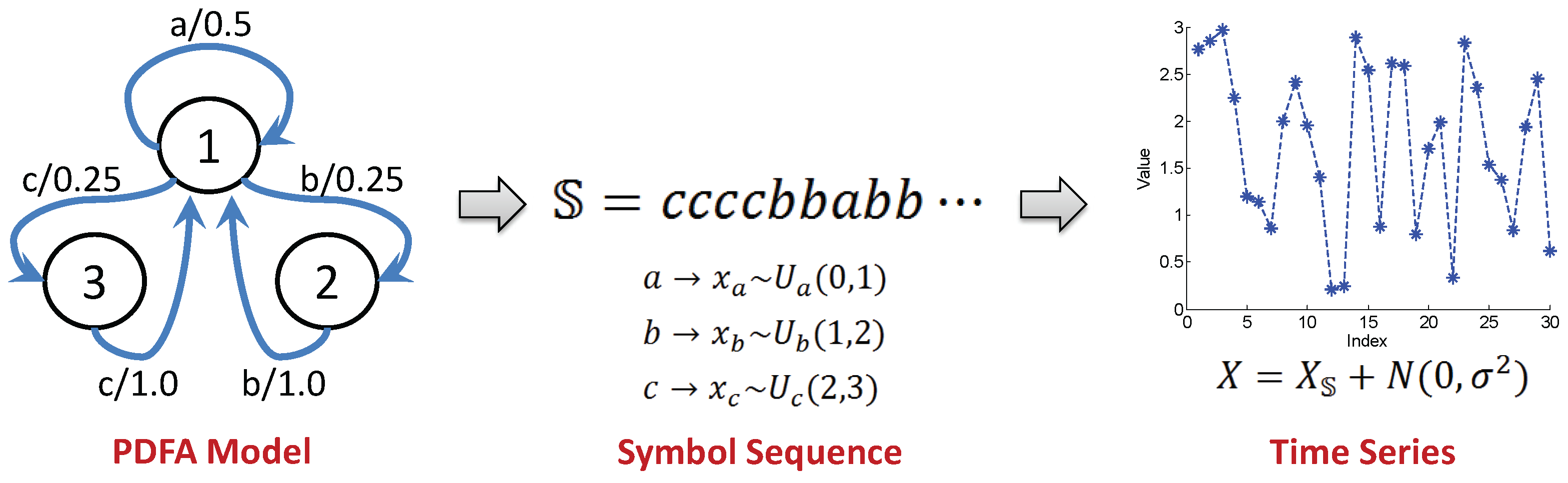
Similar to the example in [6], the PFSA in Figure 5 is a variation of the even shift machine with three symbols, i.e., , which is not a shift of finite type [8,31], because the minimal set of forbidden words has a subset , which does not have a finite cardinality. A symbol string, generated from the PFSA , is converted into a time series of real numbers by assigning uniform distribution to each symbol over the corresponding partitioning segment.
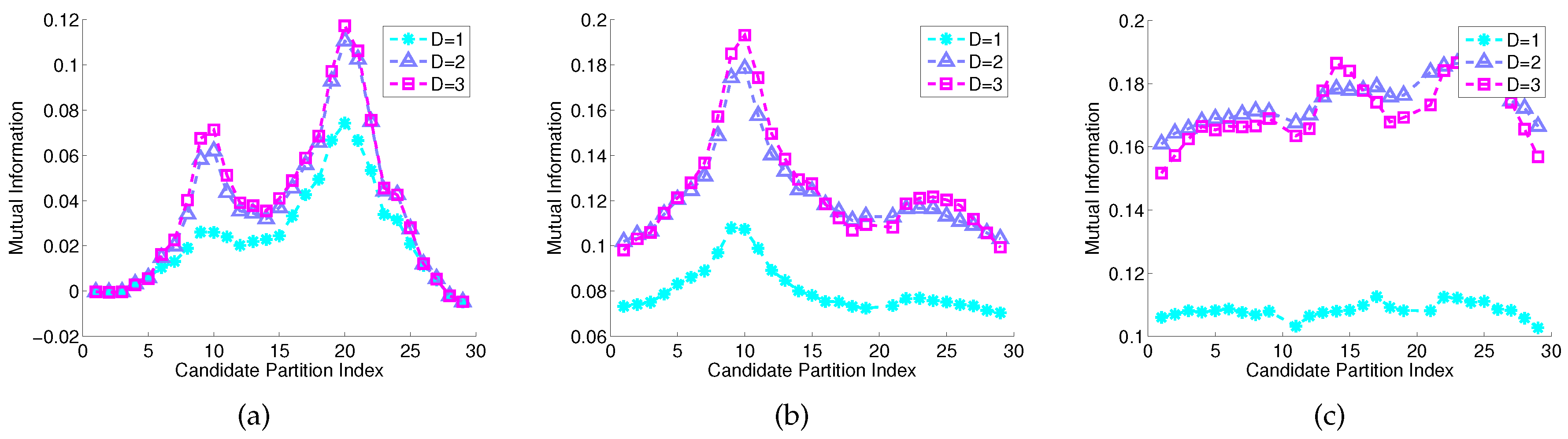
Having 30 partitioning regions as the initial guess, the time series is segmented by 29 boundary locations as seen in Figure 6 that depicts the 29 candidate locations generated by the MEP algorithm. These locations are further tuned by the proposed symbolization algorithm. Figure 7 depicts three consecutive iterations in the selection of partitioning locations via maximization of mutual information at each iteration. At the first iteration, the maximum mutual information is attained at the 19th location with a value of at depth . The maximum mutual information at for the same location is numerically very close to that at . After the 19th location is selected in the first iteration, the remaining 28 locations are analyzed in the second iteration with alphabet size of . At this stage, the values of maximum mutual information at and are very close to each other for each location, which are significantly larger than the corresponding values at . The maximum mutual information at 10th location is found to be , which is improvement of mutual information measurement compared to that for . Finally, at the third iteration with , the maximum mutual information is , which is smaller than that at ; this is possibly due to finite length of the time series. Therefore the alphabet size which achieves the maximum mutual information value is and the resulting partition is obtained as . Comparing it with the distribution assignment to each symbol, the selected partition correctly captures the temporal transition pattern from the generating process.
Table 1 presents probabilities of states and conditional emission probabilities of symbol emission, generated from the state splitting algorithm, where the top row consists of the three symbols a, b, and c; the first column from left represents the set of states; and the second column represents the respective state probabilities that sum to 1. The remaining three columns in Table 1 represent the probabilities of the respective symbols a, b, and c, conditioned on the individual states, which determine the symbol emission rule in the PFSA model.
As seen in Table 1, the three states a, , and have relatively high probabilities that are highlighted in bold in the second column. Conditioned on the state , the symbol b has a large emission probability of , which is highlighted in bold; a similar situation arises for symbol c conditioned on the state .
5.2. Experimental Validation in a Laboratory Environment
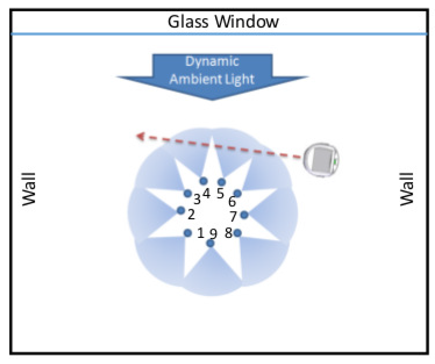
This subsection presents laboratory experimentation to demonstrate the efficacy of the proposed method for reliable (e.g., with low false-alarm rates) detection of a target in uncertain and dynamic environments [32]. Figure 8 depicts the layout of the laboratory apparatus, where a network is configured as a ring of nine infrared sensors and a computer-instrumented & computer-controlled Khepera III mobile robot (version 2.1) [33] that serves as a single moving target; details of the collected time-series data characteristics are reported in [32]. In these experiments, the dynamic environment and the associated environmental disturbances are emulated as variations in the daylight intensities on partially cloudy days. As seen in Figure 8, the local-area sensor network is placed at the center of a square room in which only one wall has open windows that are exposed to the sun. For a more detailed description of the laboratory facility, the reader is referred to the website http://nrsl.mne.psu.edu of Networked Robotic Systems Laboratory (NRSL) at Penn State.
All experiments have been conducted during days under partially cloudy conditions, where the sunlight is intermittently blocked by clouds. During the experiments, the moving target travels at a constant speed in straight lines between the sensor network and the ambient light source, as illustrated in Figure 8. The infrared sensors are oriented toward the moving target and are subjected to disturbances when the target is moving in and out, which causes intermittent blocking of the ambient light source. Due to the orientation of sensors, effects of the environment are different for individual sensors. Sensors that face the windows (i.e., the ambient light source) would have different levels of reading when compared with the rest of the sensors. When the target (i.e., the Khepera III mobile robot) is moving in, ambient light sources are partially blocked for some of the sensors, which increases their readings temporarily. Changes in the ambient light affect the moving target as the readings of some of the sensors fluctuate more significantly.
5.2.1. Data Collection
The experiments make use of measurements of the ambient light, and the performance of environmental surveillance is inherently dependent on the maximum sensor updating rates. The update time between measurements of all 9 sensors is 33 ms. During this 33 ms interval, the 9 sensors are read in a sequential way at every 3 ms. In this experimental apparatus, the central workstation is linked with sensor nodes via Bluetooth. After receiving each new measurement, the station converts and stores the sensor readings before collecting new data. Due to processing and communication delays, the average interval between two consecutive readings is ∼65.3 ms with standard deviation of ms, which makes the average updating frequency as ∼18.5 Hz with standard deviation of ∼2.9 Hz.
Figure 8 depicts layout of the experimentation. The sensor network is placed at the center of a square room in which only one wall has open windows that are exposed to the sun. All experiments have been conducted during days under partially cloudy conditions, where the sunlight is intermittently blocked by clouds. Due to the orientation of sensors, the effects of the environment are different for those of the individual sensors. Sensors which are facing the windows (i.e., the ambient light source) would have different levels of reading when compared with the rest of the sensors. Changes in the ambient light affect the moving target as the readings of some of the sensors fluctuate more significantly.
5.2.2. Consensus Partitioning among Multiple Time Series
To overcome the different environmental impacts (i.e., noise level) to different sensors, we proposed a consensus partition position selection algorithm for multiple time series based on the Algorithm 3. During the sequential selection of partitioning portions, the criterion for selection of partitioning locations is revised to choose the candidate that maximizes the average mutual information over the ensemble of time series. The only information needed to be exchanged at each iteration is the candidate index and the corresponding values of maximum mutual information. The detailed procedure for consensus partition is described in Algorithm 4.
| Algorithm 4 Consensus Partition Position Selection for Multiple Time Series |
| Require: Multiple time series , Alphabet size , and number m of candidates for a partitioning position. |
| Ensure: Partition position vector and the average maximum mutual information among all time series for the given alphabet size . |
| 1: Create a set of candidate partitioning locations via MEP (Algorithm 1) for k-th time series. |
| 2: for n=2 to do |
3:
|
| 4: The specific partitioning locations , corresponding to the the maximum mutual information , are removed from for each time series and is included in the set of selected partitioning locations to construct the optimal . |
| 5: end for |
5.2.3. Results
The results are presented for 50 experiments. For each experiment, the nine sensors in Figure 8 record synchronized data for about 65 s with a sampling rate of ∼18.5 Hz.
Since the orientation and location of sensors are diverse in the individual experiments, the time series from each sensor varies relative to each other, even for sensors under the same dynamic environment. Figure 9 presents an example of the partitioning results for sensors 1, 2, and 3 at one experiment event. In this case, three sensors have different noise-impact levels from the environment. Besides the proposed maximum mutual information partition (MMIP), the partitioning performance has been compared with two other methods: maximum entropy partitioning (MEP) and uniform space partitioning (USP).
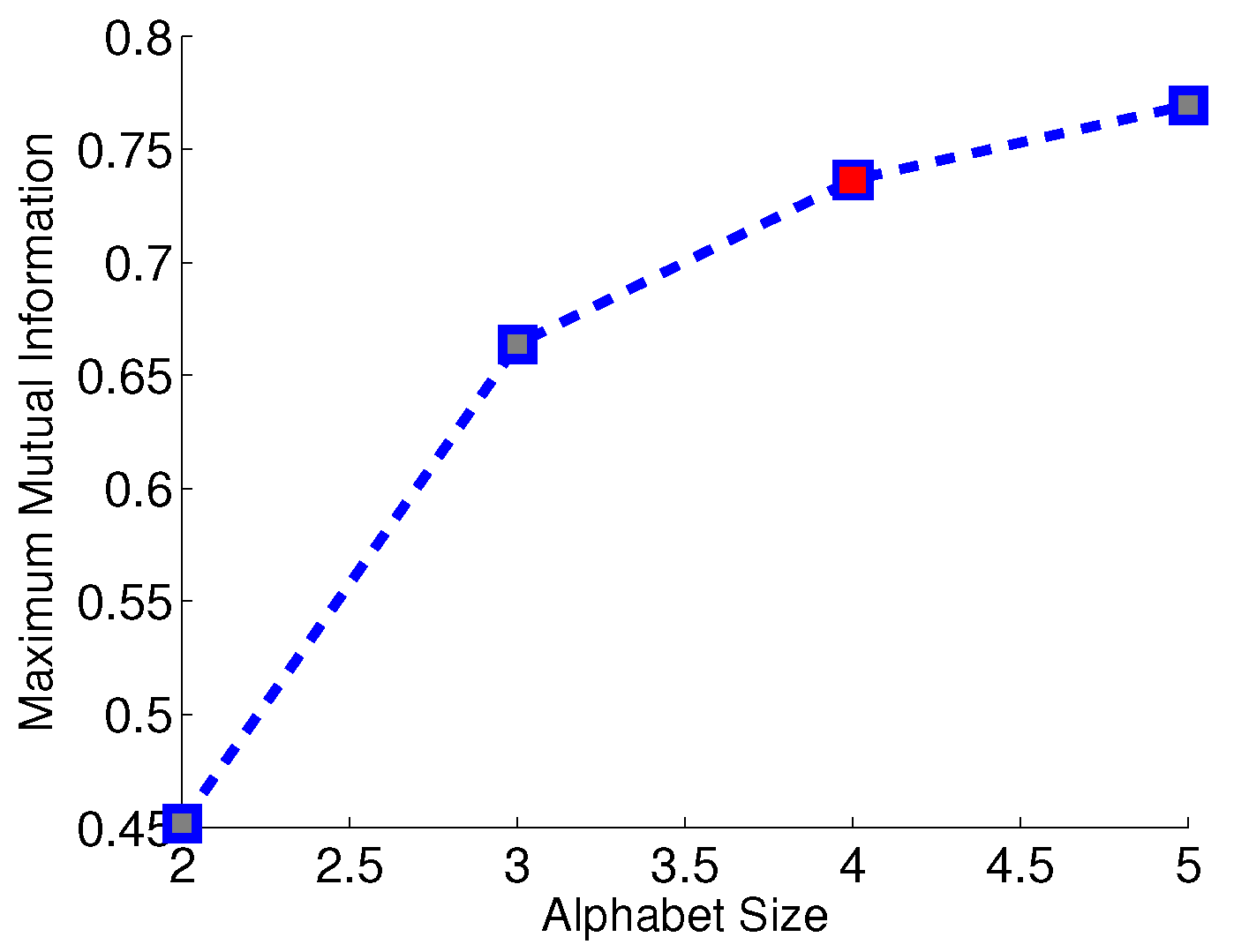
For each experiment, the overall Hamming distance among all 9 sensors is calculated as the criterion of evaluating the partitioning performance. Similarities among symbol strings from different sensors reflect the nature of underlying environmental events. Although each sensor has different location and orientation, the dynamic patterns embedded in the symbol strings are lumped together as if there is only one type of environmental noise (i.e., in the absence of a moving target). If there is a moving target in the vicinity, the challenge is to discriminate the signal characteristics from those in the absence of a target. To address this issue, a binary-tree agglomerative hierarchical clustering algorithm is adopted in this paper. The distance between two symbol strings is measured by the Hamming distance defined in Equation (6), and the distance between two clusters of symbol strings is measured by the cluster distance defined in Equation (7). The choice of the alphabet size is obtained by Subtask 1 of the proposed method. Then, the same alphabet size is used in other partitioning algorithms. Figure 10 depicts the average maximum mutual information over nine sensors for different choices of the alphabet size . The ratio of maximum mutual information for and is approximately , which is greater than the predefined threshold 0f 0.95; therefore is chosen as the selected alphabet size; this is indicated by the red fill-in of a little square in Figure 10.
The maximum Hamming distance among all nine sensors for the proposed unsupervised symbolization algorithm is , that for the maximum entropy partitioning (MEP) algorithm is , which is more than twice the distance compared to the proposed method. For the uniform space partitioning (USP) algorithm, the corresponding Hamming distance is , which is the largest among the three partitioning algorithms. That is, the proposed symbolization method achieves the smallest Hamming distance based on the symbol strings generated under different environmental impacts. The symbolization algorithm produces a small alphabet size as a result. Among the 50 experiments with (no target) environmental dynamic noise, there are 9 cases with , 39 cases with , and 2 cases with . The average Hamming distance among all 9 sensors for the proposed algorithm is , compared to for MEP and for USP. On the other hand, as for the 50 experiments with target being present, there are 18 cases with , 26 cases with , and 6 cases with . The average Hamming distance among all 9 sensors for the proposed algorithm is , compared to for MEP and for USP. It shows that the proposed algorithm significantly reduces the difference of performance among generated symbol sequences from sensor time series under different conditions. In addition, the ratio of average Hamming distance between target signal and dynamic environmental noise of the proposed method is significantly higher as compared to the other two methods, namely, MEP and USP. Thus, the dominant temporal pattern of environment, dynamics embedded in different time series, is magnified.
6. Conclusions and Future Work
This paper has developed an unsupervised algorithm for symbolization of time series. The objective is to model the embedded temporal behavior as a probabilistic deterministic finite-state automaton (PFSA) in an information-theoretic Markov setting. The results are obtained by maximizing the mutual information between symbols and states; consequently, the uncertainty of the constructed model is reduced. In this context, three main issues are addressed:
- Determination of the symbol alphabet size .
- Identification of the boundary locations for partitioning, , of the time series.
- Identification of the state set in the PFSA model.
The symbolization algorithm has been validated on time series data generated by both numerical simulation and laboratory experimentation. It is observed that the proposed algorithm outperforms two standard time series symbolization algorithms, namely, maximum entropy partitioning (MEP) and uniform space partitioning (USP).
While there are many other issues that need to resolved by further theoretical and experimental research, the authors suggest the following topics for future research:
- Vector time series: Generalization of the proposed symbolization algorithm from scalar-valued (i.e., one dimensional) time series to vector-valued (i.e., multi-dimensional) time series.
- Extension of the proposed symbolization method for information extraction from time series: One such potential approach is the usage of ordinal patterns [34] in the symbolized time series, which defines symbols into characteristic zones, instead of partitioning the full data range.
- Investigation of the effects of the sampling rate on partitioning of the time series: The choice of symbols and states is influenced by the sampling rate of data acquisition. It is necessary to establish an adaptive algorithm that will allow autonomous downsampling or upsampling of time series before symbolization.
- Threshold parameters, and : Quantitative evaluation of these parameters as inputs to Equation (16) and Algorithm 2.
- Suboptimality of greedy search: Quantification of estimated losses in the proposed greedy search algorithm with respect to an optimal or near-optimal algorithm.
- Comparative evaluation: Extensive investigation to further evaluate the proposed method for comparison with other reported work on symbolization of time series (e.g., Symbolic Aggregate approXimation (SAX) [35]).
Acknowledgments
This work has been supported in part by the U.S. Air Force Office of Scientific Research (AFOSR) under Grant No. FA9550-15-1-0400. Any opinions, findings and conclusions or recommendations expressed in this publication are those of the authors and do not necessarily reflect the views of the sponsoring agencies.
Author Contributions
Yue Li and Asok Ray conceived and designed the experiments; Yue Li performed the experiments; Yue Li and Asok Ray analyzed the data; Asok Ray and Yue Li wrote the paper. Both authors have read and approved the final manuscript.
Conflicts of Interest
The authors declare no conflict of interest.
References
- Hadamard, J. Les surfaces à courbures opposées et leurs lignes géodésique. J. Math. Pures Appl. 1898, 4, 27–73. [Google Scholar]
- Shannon, C.E. A mathematical theory of communication. ACM SIGMOBILE Mob. Comput. Commun. Rev. 2001, 5, 3–55. [Google Scholar] [CrossRef]
- Lin, J.; Keogh, E.; Lonardi, S.; Chiu, B. A symbolic representation of time series, with implications for streaming algorithms. In Proceedings of the 8th ACM SIGMOD wOrkshop on Research Issues in Data Mining and Knowledge Discovery, San Diego, CA, USA, 13 June 2003; pp. 2–11. [Google Scholar]
- Daw, C.S.; Finney, C.E.A.; Tracy, E.R. A review of symbolic analysis of experimental data. Rev. Sci. Instrum. 2003, 74, 915–930. [Google Scholar] [CrossRef]
- Ray, A. Symbolic dynamic analysis of complex systems for anomaly detection. Signal Process. 2004, 84, 1115–1130. [Google Scholar] [CrossRef]
- Mukherjee, K.; Ray, A. State splitting and merging in probabilistic finite state automata for signal representation and analysis. Signal Process. 2014, 104, 105–119. [Google Scholar] [CrossRef]
- Martin, L.; Puterman, M.L. Markov Decision Processes: Discrete Stochastic Dynamic Programming; Wiley: Hoboken, NJ, USA, 2014. [Google Scholar]
- Lind, D.; Marcus, B. An Introduction to Symbolic Dynamics and Coding; Cambridge University Press: Cambridge, UK, 1995. [Google Scholar]
- Rajagopalan, V.; Ray, A. Symbolic time series analysis via wavelet-based partitioning. Signal Process. 2006, 86, 3309–3320. [Google Scholar] [CrossRef]
- Graben, P.B. Estimating and improving the signal-to-noise ratio of time series by symbolic dynamics. Phys. Rev. E 2001, 64, 051104. [Google Scholar] [CrossRef] [PubMed]
- Piccardi, C. On the control of chaotic systems via symbolic time series analysis. Chaos 2004, 14, 1026–1034. [Google Scholar] [CrossRef] [PubMed]
- Alamdari, M.M.; Samali, B.; Li, J. Damage localization based on symbolic time series analysis. Struct. Control Health Monit. 2015, 22, 374–393. [Google Scholar] [CrossRef]
- Sarkar, S.; Chattopadhyay, P.; Ray, A. Symbolization of dynamic data-driven systems for signal representation. Signal Image Video Process. 2016. [Google Scholar] [CrossRef]
- Kennel, M.B.; Mees, A.I. Context-tree modeling of observed symbolic dynamics. Phys. Rev. E 2002, 66, 056209. [Google Scholar] [CrossRef] [PubMed]
- Takens, F. Detecting Strange Attractors in Turbulence; Springer: Berlin/Heidelberg, Germany, 1981. [Google Scholar]
- Rissanen, J. A universal data compression system. IEEE Trans. Inf. Theory 1983, 29, 656–664. [Google Scholar] [CrossRef]
- Ahmed, A.M.; Bakar, A.A.; Hamdan, A.R. Dynamic data discretization technique based on frequency and k-nearest neighbour algorithm. In Proceedings of the 2nd Conference on Data Mining and Optimization, DMO’09, Pekan Bangi, Malaysia, 27–28 October 2009; pp. 10–14. [Google Scholar]
- Bishop, C.M. Pattern Recognition and Machine Learning (Information Science and Statistics); Springer: New York, NY, USA; Secaucus, NJ, USA, 2006. [Google Scholar]
- Lehrman, M.; Rechester, A.B.; White, R.B. Symbolic analysis of chaotic signals and turbulent fluctuations. Phys. Rev. Lett. 1997, 78, 54. [Google Scholar] [CrossRef]
- Mörchen, F.; Ultsch, A. Optimizing time series discretization for knowledge discovery. In Proceedings of the Eleventh ACM SIGKDD International Conference on Knowledge Discovery in Data Mining, Chicago, IL, USA, 21–24 August 2005; pp. 660–665. [Google Scholar]
- Kullback, S.; Leibler, R.A. On information and sufficiency. Ann. Math. Stat. 1951, 22, 79–86. [Google Scholar] [CrossRef]
- Barron, A.; Rissanen, J.; Yu, B. The minimum description length principle in coding and modeling. IEEE Trans. Inf. Theory 1998, 44, 2743–2760. [Google Scholar] [CrossRef]
- Willems, F.M.J.; Shtarkov, Y.M.; Tjalkens, T.J. The context-tree weighting method: basic properties. IEEE Trans. Inf. Theory 1995, 41, 653–664. [Google Scholar] [CrossRef]
- Darema, F. Dynamic data driven applications systems: New capabilities for application simulations and measurements. In Proceedings of the 5th International Conference on Computational Science—ICCS 2005, Atlanta, GA, USA, 22–25 May 2005. [Google Scholar]
- Crochemore, M.; Hancart, C. Automata for matching patterns. In Handbook of Formal Languages; Springer: Berlin/Heidelberg, Germany, 1997; Volume 2, Chapter 9; pp. 399–462. [Google Scholar]
- Béal, M.P.; Perrin, D. Symbolic dynamics and finite automata. In Handbook of Formal Languages; Springer: Berlin/Heidelberg, Germany, 1997; Volume 2, Chapter 10; pp. 463–506. [Google Scholar]
- Sipser, M. Introduction to the Theory of Computation; Cengage Learning: Boston, MA, USA, 2012. [Google Scholar]
- Palmer, N.; Goldberg, P.W. Pac-learnability of probabilistic deterministic finite state automata in terms of variation distance. Theor. Comput. Sci. 2007, 387, 18–31. [Google Scholar] [CrossRef]
- Cover, T.M.; Thomas, J.A. Elements of Information Theory; Wiley: Hoboken, NJ, USA, 2012. [Google Scholar]
- Feldman, D.P. A Brief Introduction to: Information Theory, Excess Entropy and Computational Mechanics; College of the Atlantic: Bar Harbor, ME, USA, 2002; Volume 105, pp. 381–386. [Google Scholar]
- Dupont, P.; Denis, F.; Esposito, Y. Links between probabilistic automata and hidden markov models, probability distributions, learning models and induction algorithms. Pattern Recognit. 2005, 38, 1349–1371. [Google Scholar] [CrossRef]
- Li, Y.; Jha, D.K.; Ray, A.; Wettergren, T.A. Information fusion of passive sensors for detection of moving targets in dynamic environments. IEEE Trans. Cybern. 2017, 47, 93–104. [Google Scholar] [CrossRef] [PubMed]
- Robot, K., III. User Manual, version 2.1. Available online: https://www.k-team.com/mobile-robotics-products/khepera-iii (accessed on 30 March 2017).
- Kulp, C.W.; Chobot, J.M.; Freitas, H.R.; Sprechini, G.D. Using ordinal partition transition networks to analyze ecg data. Chaos 2016, 26, 073114. [Google Scholar] [CrossRef] [PubMed]
- Malinowski, S.; Guyet, T.; Quiniou, R.; Tavenard, R. 1d-sax: A novel symbolic representation for time series. In Proceedings of the International Symposium on Intelligent Data Analysis, IDA2013: Advances in Intelligent Data Analysis XII, London, UK, 17–19 October 2013; pp. 273–284. [Google Scholar]
Figure 1.
An example of time series symbolization: First, a single partition boundary is applied to the original time series; then, each signal is mapped to the symbol which is associated to the region; finally, the state is generated by combining symbol blocks.
Figure 1.
An example of time series symbolization: First, a single partition boundary is applied to the original time series; then, each signal is mapped to the symbol which is associated to the region; finally, the state is generated by combining symbol blocks.

Figure 2.
Maximum Shannon entropy (shown by blue square) and entropy excess (shown by red triangle) for different alphabet sizes . The unit for each of Shannon entropy and entropy excess is the natural unit of information (i.e., nat).
Figure 2.
Maximum Shannon entropy (shown by blue square) and entropy excess (shown by red triangle) for different alphabet sizes . The unit for each of Shannon entropy and entropy excess is the natural unit of information (i.e., nat).
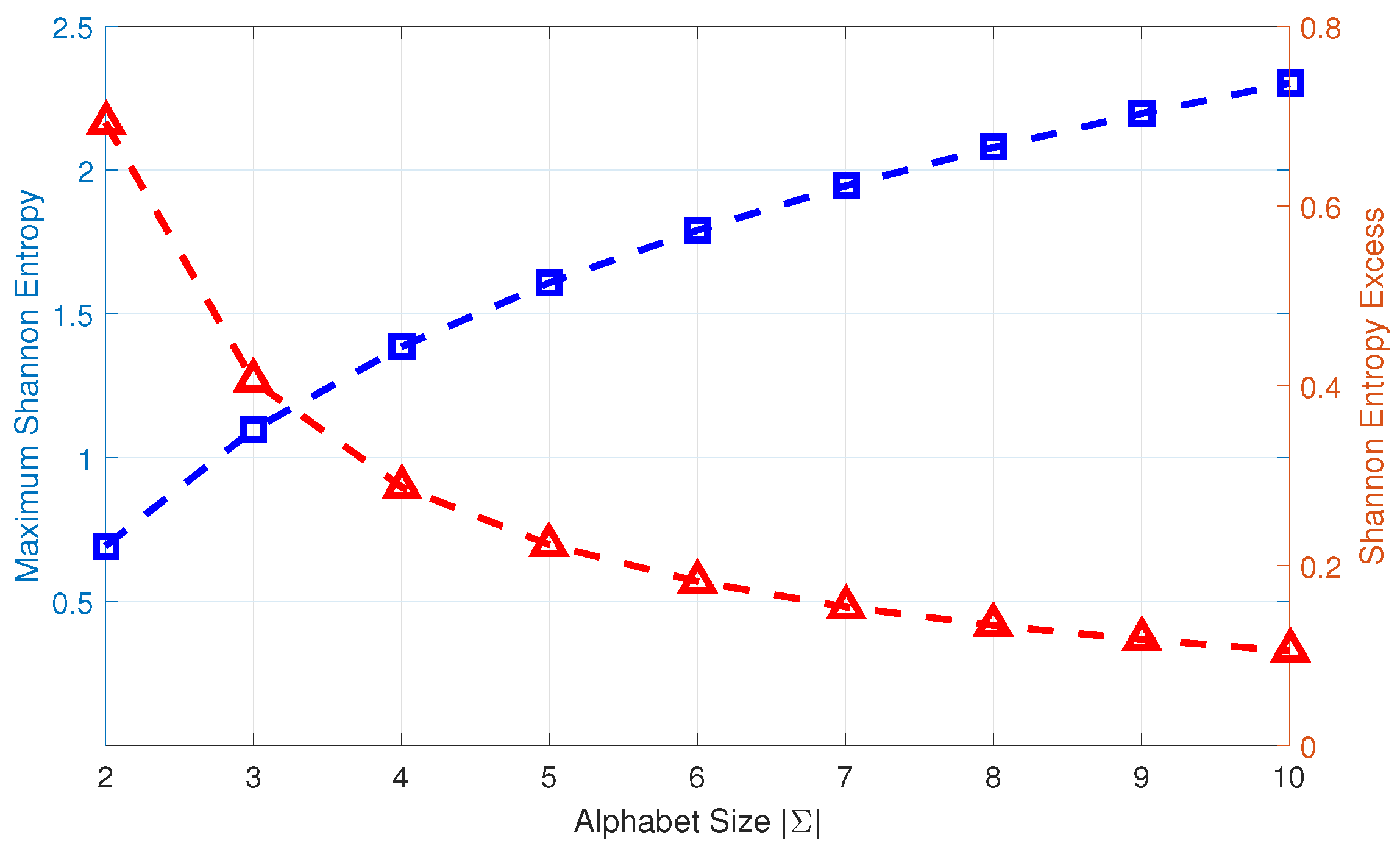
Figure 3.
Relationship among three subtasks. Subtask 1 is necessary for Subtask 2, and both Subtask 1 and Subtask 2 are necessary for Subtask 3.
Figure 3.
Relationship among three subtasks. Subtask 1 is necessary for Subtask 2, and both Subtask 1 and Subtask 2 are necessary for Subtask 3.

Figure 4.
An example of state splitting with alphabet . The state q is first split as . The new state is not further split, because its occurrence probability is less than the threshold . The new state is not further split because the sum of conditional entropy of generated states is not significantly reduced compared to that of state . The state is split as both criteria are satisfied. States after splitting are .

Figure 5.
Example of simulation validation via time series generated from a PFSA model.

Figure 6.
An example of 29 candidate partitioning locations for the simulation time series generated from probabilistic finite-state automata (PFSA).
Figure 6.
An example of 29 candidate partitioning locations for the simulation time series generated from probabilistic finite-state automata (PFSA).
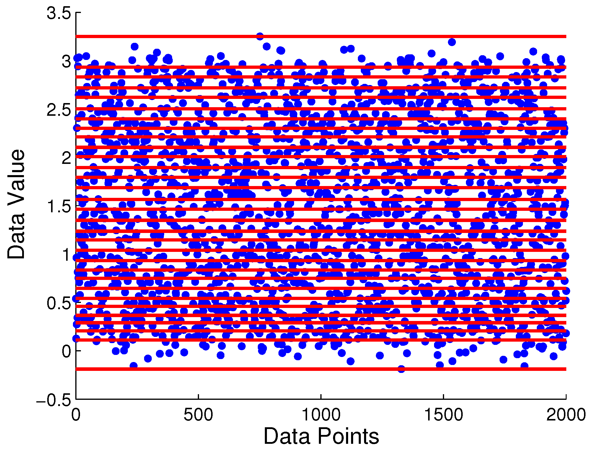
Figure 7.
Mutual information for each candidate partitioning locations for each iteration at different depth D of the PFSA model. The unit for mutual information is the natural unit of information (i.e., nat). (a) 1st iteration, & ; (b) 2nd iteration, & ; (c) 3rd iteration, & .
Figure 7.
Mutual information for each candidate partitioning locations for each iteration at different depth D of the PFSA model. The unit for mutual information is the natural unit of information (i.e., nat). (a) 1st iteration, & ; (b) 2nd iteration, & ; (c) 3rd iteration, & .

Figure 8.
Experimental setup for target detection in a dynamic environment.

Figure 9.
Three different types of partitioning, namely, the proposed maximum mutual information partitioning (MMIP), maximum entropy partitioning (MEP), and uniform space sartitioning (USP) for time series of sensors 1, 2, and 3. Plots (a–c) represent sensor No. 1; plots (d–f) represent sensor No. 2; and plots (g–i) represent sensor No. 3. The alphabet size for each case is , which is obtained by Subtask 1. The partitioning line segments for symbolization are shown by (red) dashed horizontal lines and time series of sensors are marked in (blue) solid-line profiles.
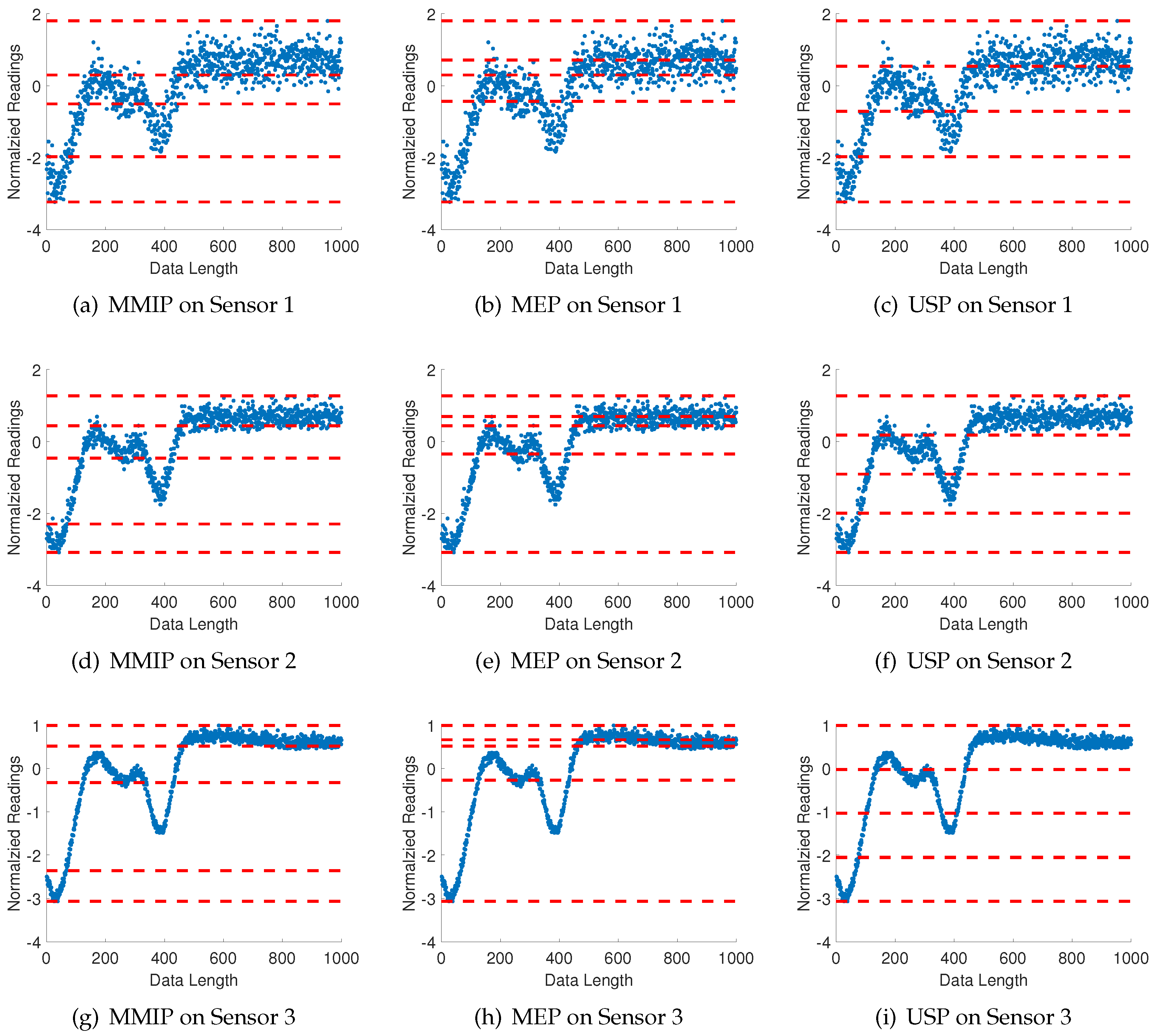
Figure 10.
Average maximum mutual information over 9 sensors for different alphabet sizes. is chosen as the selected alphabet size as marked in red. The unit for mutual information is the natural unit of information (i.e., nat).
Figure 10.
Average maximum mutual information over 9 sensors for different alphabet sizes. is chosen as the selected alphabet size as marked in red. The unit for mutual information is the natural unit of information (i.e., nat).


Table 1.
Matrix of probabilities of symbol emission conditioned on state occurrence.
| Alphabet | a | b | c | ||
|---|---|---|---|---|---|
| a | |||||
| State | |||||
© 2017 by the authors. Licensee MDPI, Basel, Switzerland. This article is an open access article distributed under the terms and conditions of the Creative Commons Attribution (CC BY) license (http://creativecommons.org/licenses/by/4.0/).
Share and Cite
MDPI and ACS Style
Li, Y.; Ray, A. Unsupervised Symbolization of Signal Time Series for Extraction of the Embedded Information. Entropy 2017, 19, 148. https://doi.org/10.3390/e19040148
AMA Style
Li Y, Ray A. Unsupervised Symbolization of Signal Time Series for Extraction of the Embedded Information. Entropy. 2017; 19(4):148. https://doi.org/10.3390/e19040148
Chicago/Turabian StyleLi, Yue, and Asok Ray. 2017. "Unsupervised Symbolization of Signal Time Series for Extraction of the Embedded Information" Entropy 19, no. 4: 148. https://doi.org/10.3390/e19040148
Note that from the first issue of 2016, this journal uses article numbers instead of page numbers. See further details here.