Structure and Dynamics of Water at Carbon-Based Interfaces


1
Department of Physics, Technical University of Catalonia—Barcelona Tech, B5-209 Northern Campus, 08034 Barcelona, Spain
2
Secció de Física Estadística i Interdisciplinària, Departament de Física de la Matèria Condensada, Facultat de Física, Universitat de Barcelona, Martí i Franquès 1, 08028 Barcelona, Spain
3
Institute of Nanoscience and Nanotechnology (IN2UB), Universitat de Barcelona, Av. Joan XXIII S/N, 08028 Barcelona, Spain
*
Authors to whom correspondence should be addressed.
Entropy 2017, 19(3), 135; https://doi.org/10.3390/e19030135
Submission received: 9 March 2017
/
Revised: 19 March 2017
/
Accepted: 19 March 2017
/
Published: 21 March 2017
(This article belongs to the Special Issue Nonequilibrium Phenomena in Confined Systems)
Abstract
:Water structure and dynamics are affected by the presence of a nearby interface. Here, first we review recent results by molecular dynamics simulations about the effect of different carbon-based materials, including armchair carbon nanotubes and a variety of graphene sheets—flat and with corrugation—on water structure and dynamics. We discuss the calculations of binding energies, hydrogen bond distributions, water’s diffusion coefficients and their relation with surface’s geometries at different thermodynamical conditions. Next, we present new results of the crystallization and dynamics of water in a rigid graphene sieve. In particular, we show that the diffusion of water confined between parallel walls depends on the plate distance in a non-monotonic way and is related to the water structuring, crystallization, re-melting and evaporation for decreasing inter-plate distance. Our results could be relevant in those applications where water is in contact with nanostructured carbon materials at ambient or cryogenic temperatures, as in man-made superhydrophobic materials or filtration membranes, or in techniques that take advantage of hydrated graphene interfaces, as in aqueous electron cryomicroscopy for the analysis of proteins adsorbed on graphene.
1. Introduction
The knowledge of microscopic properties of confined water is of central importance in a wide range of physical systems and processes such as electrochemical systems [1,2], corrosion [3,4], solar energy conversion [5], energy-harvesting and generation devices [6], meteorology [7] or in a wide variety of biosystems (lipid membranes, proteins, etc.) [8,9], including protein adsorbed on graphene at cryogenic temperatures [10], to mention only a few. It has been found that microscopic structure, dielectric properties and dynamics of water suffer important changes when water is close to solid or liquid interfaces [11]. Further, significant changes in the thermodynamical stability limits of constrained water have been also verified [12,13], including evidences of crystallization promotion/inhibition from simulations [14,15,16,17,18,19].
In theoretical and computational works, effective potentials have been usually employed to model water-surface interactions in terms of Van der Waals forces accounted mostly with Lennard-Jones 6–12 potentials, where the typical parameters for carbon-oxygen and carbon-hydrogen forces are normally adapted with the help of Lorentz–Berthelot rules [20,21,22,23,24]. A variety of solid surfaces has been considered: silica pores (Vycor glass) [25,26], platinum [27], magnetite [28], zirconia [29], or pure carbon composites (graphite structure) in several geometries, from planar [30,31,32,33,34] to cylindrical [35,36,37]. At the experimental side, many authors have contributed to the study of water at hydrophobic interfaces using a wide variety of techniques such as scanning tunneling microscopy [38], environmental scanning electron microscopy and electron energy loss spectroscopy [39], ultrafast optical Kerr effect spectroscopy [40], atomic force spectroscopy [41], calorimetry [42], neutron diffraction [43,44,45,46] and electron cryomicroscopy [10].
Here we consider liquid water constrained by variety of setups corresponding to two different geometries, namely carbon nanotubes (CNTs) and flat graphene sheets. In all cases, we analyze a wide range of thermodynamical conditions, including ambient-like, supercritical and near-melting. In particular, the calculations of the water adsorption free energies, the thermodynamical stability of the phases and the diffusion of confined water, show important changes depending on the curvature of the interface. These results are interesting for understanding possible applications of nanostructured carbon-based surfaces as, for example, in anti-fogging or self-cleaning materials [47]. We also show new results about the crystallization and evaporation of water confined between parallel walls at sub-nanometric distances. We find that the diffusion changes in a non-monotonic way for decreasing confining distances. These results could be relevant for the design of nanometric membranes able to filter ions out of water [48].
2. Liquid Water on Carbon-Based Interfaces
Gordillo and Martí recently studied [49] TIP3P water at the exterior surface of cylindrical CNTs. It is interesting to compare the results under these conditions with the case of water on a single, rigid and flat graphene sheet. Carbon nanotubes are cylinders that can be considered as the result of “cutting” a strip on a graphene sheet and rolling it up in such a way as to leave no dangling bonds [50]. Since the strip can be cut with any orientation, this method can produce different kinds of CNTs with different radii. Here we consider only those of the (n,n) type in the standard nomenclature [51] reported in Table 1.
2.1. Thermodynamic Stability
In order to perform a meaningful study of the adsorption of water on CNTs and graphene, Calero et al. [52] determine the limiting densities for the thermodynamic stability of a coat of water on those substrates. For a given phase, a thermodynamically stable layer of water uniformly covers the substrate without denser or sparser regions. To evaluate which conditions guarantee this stability, they calculate the free energy of the system and perform, if necessary, a Maxwell construction between coexisting phases. To this goal they follow a procedure previously established in other works [36,49] and based on the calculation of the energy per particle E by Molecular Dynamics (MD) simulation in the ensemble, as described in the Computational Methods section. First they propose a functional form for the Helmholtz free energy as a function of the surface density ρ and the temperature T,
where the terms corresponding to the ideal gas is dropped and where are fitting parameters. They extract these parameters from a least squares fitting procedure of
calculated by simulations at different densities and temperatures (Figure 1). For each CNT they consider as a reference surface for the calculation of the water density a cylinder with a radius corresponding to the first peak of the water radial density profile and the axis and length coinciding with those of the CNT. For the graphene the reference surface is the area of the flat sheet. The good quality () of the fits in Figure 1 allows them to limit to two the order of the density polynomial in Equation (2), at variance with the choice of [36,49]. Moreover, here a single fit accounts for the entire density-dependence of E, because E is a monotonic function of ρ, in contrast with the results in [36] where two independent fits in different density ranges are necessary for the appearance of two local minima in .
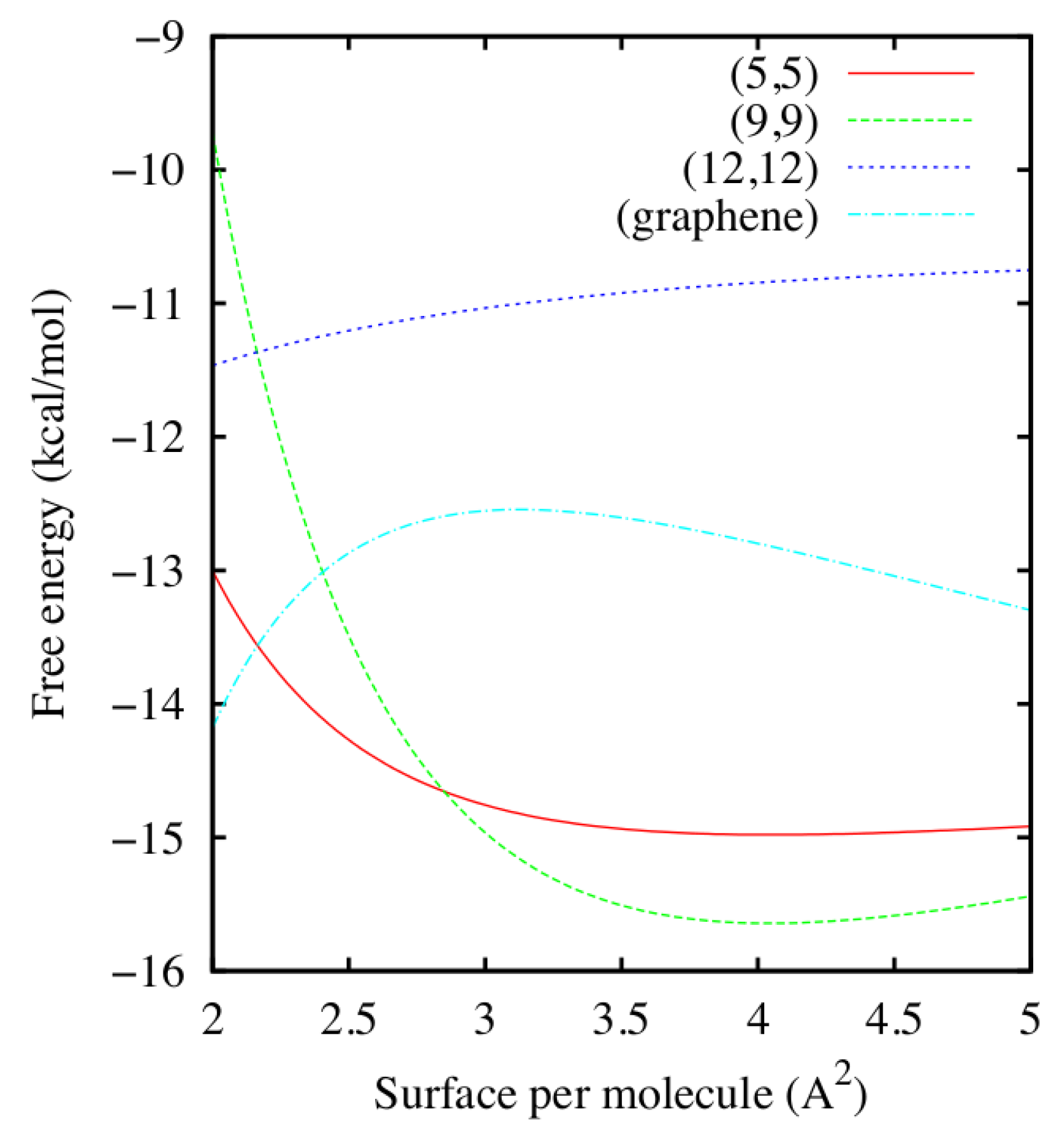
Once the coefficients are known, Calero et al. [52] compute in Equation (1), as reported in Figure 2 for K. Curves for and 323 K (not shown) are similar to those for 298 K, but displaced to lower values of F. From the the minima and the shape of F as function of ρ and T one can evaluate the stability of the adsorbed water layer.
We observe that for the (9,9) and (5,5) CNTs F has a minimum at ≈ 4.05 Å2, corresponding to ≈ 905 and 790 water molecules around each CNT, respectively, and ≈ 7.4 × 10⁻⁸ g/cm2 > 3 × 10⁻⁸ g/cm2 of the bulk at volumic density is g/cm3. This finding implies that a stable layer of liquid water adsorbs on top of the (9,9) and (5,5) CNTs under the simulated conditions.
Conversely, for the (12,12) CNT and the graphene surface, at the same temperatures we do not observe minima of F within the range of explored densities, corresponding to values of surface per molecules between 2 Å2 and 5 Å2. Furthermore, for the considered range of densities, F has a concave shape, corresponding to thermodynamically unstable states. The fact that F must be, for thermodynamic consistency, convex over a large-enough range of densities, implies that there must be two coexisting stable phases, one at higher density and another at lower density than those explored, but that they are inaccessible under the study conditions. As a consequence, in the considered range of T and ρ, there is no stable layer of liquid water adsorbed on top of the (12,12) CNT or the graphene sheet. This result is consistent with the findings of Werder et al. [53].
2.2. Structure and Hydrogen Bonding
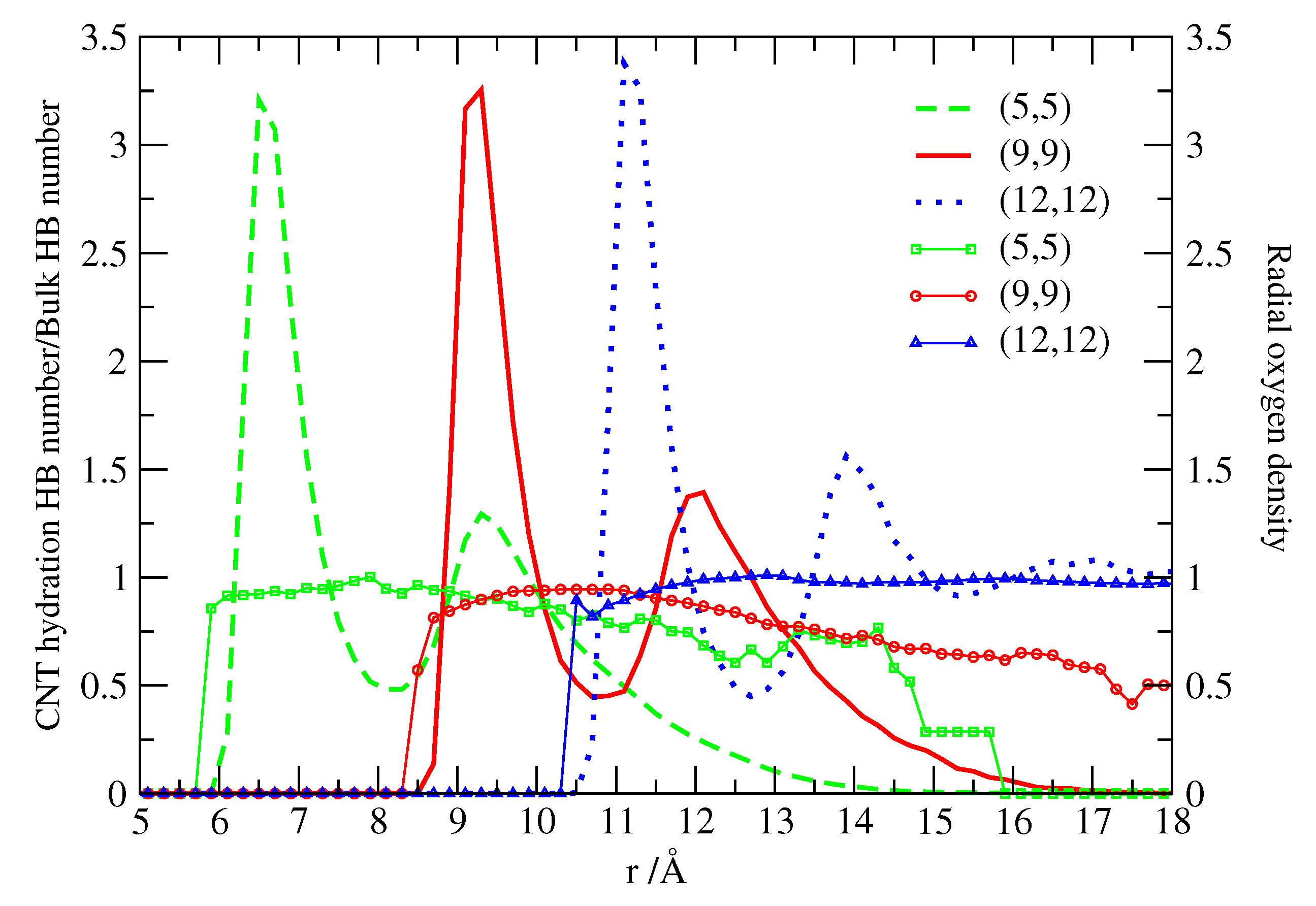
The structure of water adsorbed at the different CNTs is reported in Figure 3. Calero et al. [52] calculate the radial oxygen density profiles of water and the corresponding hydrogen-bond (HB) distributions. They adopt a geometrical definition of the HB in which two water molecules are H-bonded when their oxygen-oxygen distance is Å and the angle is < 30° [54]. The cutoff for the O-O distance corresponds to the position of the first minimum in oxygen-oxygen radial distribution functions of bulk water simulations at standard conditions. The angular cutoff corresponds to the assumption that only quasi-linear (low-energy) HBs are accounted for, while molecules in other configurations are considered as non-bonded [55]. They normalize the HB number by 3.7, that is the number of HBs formed by bulk TIP3P-water, very close to the experimental value of 3.9 [56].
We observe in all cases that at tube-water interfaces the normalized number of HBs starts below 1, corresponding to ≈ 3.5 HBs. At longer radial distances, the HB numbers rise to values closer to the bulk value, to decrease again at water-vacuum interfaces. This is qualitatively similar to what happens in other hydrophobic surfaces and in particular in the case of flat and corrugated graphene, as a consequence of the existence of dangling bonds associated to H atoms pointing directly to the surface. Therefore, the first water layer at the carbon nanotube interfaces is not able to form as many HBs as in bulk due to the existence of non-H-bonded hydrogens. However, subsequent layers can form almost as many HBs as in bulk up to reaching the water-vacuum interface, at least for (5,5) and (9,9) CNTs. For the (12,12) CNT the number of HBs at large distance does not decrease because water reaches the bulk density and there is no vacuum.
This observation is consistent with the behavior of the density profile (Figure 3) that converges toward the bulk value for the (12,12) CNT case. On the other hand, for the two smaller CNTs, (5,5) and (9,9), the density decreases with distance forming an interface between water and vacuum. For all the CNTs considered here, we observe that the density profiles mark two well defined water layers whose distance from the CNT surface is determined by the water molecular size. In fact, the ideal radius of each CNT can be calculated from its (n,m) indices as
with nm, corresponding to 3.39 Å for (5,5), 6.11 Å for (9,9), 8.14 Å for (12,12). For each CNT we find that the first water shell is at approximately 3 Å away from its surface and the second shell is centered 3 more Å away from the first. The appearance of the interfacial structure is a well known feature for water near carbon-based structures [57,58,59]. Further, the structure of water adsorbed in paraffin-like plates [60] is very similar to the one reported in Figure 3, which suggests that the key factor in determining water structure is the hydrophobic nature of the surface, independently of the particular arrangement of surface atoms.
This distribution of HB can be further understood by analyzing the orientation of water molecules at the interfaces. We calculate the average of the two first Legendre polynomials , of the angle formed by the instantaneous dipole moment of water and the direction normal to the CNT surface (Figure 4).
The first Legendre polynomial may be compared to dielectric relaxation measurements [61]. For , the second polynomial is able to discriminate between the case with water molecules randomly oriented in all directions, with , and the case with water molecules oriented at , with .
2.3. Diffusion Coefficients
2.3.1. Water inside CNTs
The diffusion of confined water is usually very different than that of bulk water [24,62,63]. Inside carbon slit-pores for instance, when it is close to the walls, water diffuses in a different fashion than at at the center of the structure [64], tending to move along planes parallel to the carbon walls. When water is inside CNTs, diffusion varies according of the CNT radius and the temperature of the system. At room temperature and for different CNTs (Table 2), Martí and coworkers [65] find that the longitudinal diffusion coefficient along z-axis is larger than the coefficient along the plane (normal plane to z). Except for the (6,6) CNT case, the overall diffusion coefficient , approximately equal to the average of the coefficients in the two directions, is slightly larger than the isotropic diffusion coefficient in the bulk case.
While is smaller the narrower is the CNT, Martí and coworkers [65] find that has a non-monotonic behavior. Specifically it decreases for CNT with diameters > 1 nm, e.g., nm for Equation (3), and increases when the diameter is nm < 1 nm. This increase of longitudinal diffusion for confining distance < 1 nm has been discussed in other works [57,66,67,68,69], finding relation with the water density under confinement [70], with controversial experimental and numerical results [59,71] and implications for the filtration of ions in water through sub-nm channels [48].
2.3.2. Water outside CNTs and on Flat Rigid Graphene
Calero et al. [52] calculate the translational self-diffusion coefficients along the axial direction of water oxygens adsorbed on the outside of CNTs and compare them with the bulk value (Table 3). In this case, they do not consider the diffusion along the radial direction because the large density reduction along such direction. They estimate by computing the long-time slopes of the mean square displacement of oxygens and using the Einstein’s relation for diffusion.
We observe that the TIP3P water model [74] considered for these calculations overestimates water diffusion in bulk by a factor 2.5, since experimental value is close to 2.3 × 10⁻⁵ cm2/s [75]. Assuming this drawback of the force field employed in the present work, one can observe from Table 3 that diffusion coefficients of water computed alongside z-axis are about 20% lower than that of the bulk unconstrained system. Therefore, the interaction of water with the CNT leads to a decrease of water diffusion parallel to the surface.
In previous works [76,77] about axial and normal diffusion of water at hydrophobic interfaces, Martí and coworkers show that water’s translational diffusion is mainly due to motion along the first interfacial layer, being the normal diffusion about one order of magnitude smaller. Here, we observe that the surface curvature does not play a relevant role in determining the self-diffusion of water on the CNT’s outside, because the diffusion reduction is approximately the same for all the considered CNTs. Furthermore, the calculations of the self-diffusion of water adsorbed on a flat graphene sheet show no relevant difference with the CNTs cases (Table 3). Therefore, we conclude that, as it happens for the structural properties of the previous section, the dynamics of the water adsorbed on the outside of a carbon surface is not strongly affected by the size and curvature of the interface.
2.3.3. Water on Corrugated Graphene
To analyze a different case of water adsorption on hydrophobic probes, Martí and coworkers [78] consider liquid water constrained on corrugated graphene sheets, as described in Section 4, and calculate the translational self-diffusion coefficient of water oxygen (i) at the surface; (ii) in the bulk-like region and (iii) at the water-vacuum interface. The calculations are made by means of time integration of the oxygen velocity autocorrelation functions computed for water molecules located in selected regions, following Berne and coworkers [79]. Previous estimates for a variety of thermodynamical states, ranging from ambient to supercritical, for water near hydrophobic surfaces [64] indicate that water molecules stay at least 2–3 ps at the interfaces or within the bulk-like region. Therefore, one can safely define the oxygen velocity autocorrelation functions for a suitable time interval (0.5–1 ps) in the selected regions and compute .
Martí and coworkers [78] consider different distortions to generate corrugated structures, as described in Section 4, and for each calculate in the three regions (Table 4). They compare the results with near a flat graphene surface. It must be noted that for this analysis they adopt a flexible-SPC water model [80]. This force field differs from those used for the studies reported in the previous sections and, in particular, has a self-diffusion coefficients for water near flat graphene, 3.3 × 10⁻⁵ cm2/s, 28% smaller than that indicated above (4.6 × 10⁻⁵ cm2/s).
Their analysis near corrugated graphene reveals a remarkable similarity for the diffusion coefficients at water-graphene interface for all corrugations types. They find that in this region water diffusion is 2.6 × 10⁻⁵–2.8 × 10⁻⁵ cm2/s in good agreement with the results reported previously [64] for narrow slit pores. This value is about 20% smaller than near a flat graphene sheet, independent on the kind of corrugation. Therefore, the interface roughness reduces water diffusion, possibly due to the hindrance caused along the surface.
Also in the central bulk like region is independent on the corrugations type. It ranges between 2.1 × 10⁻⁵–2.3 × 10⁻⁵ cm2/s, very close to the water self-diffusion coefficient for the same model in bulk [81], i.e., 2.5 × 10⁻⁵ cm2/s.
Conversely, the strongly depends on the distortion amplitude of the graphene sheet in the region that is the furthest from the surface. In this region the diffusion coefficient grows significantly with respect to the bulk-like region up to double it for the largest amplitude. This effect might be due to the important reduction in the number of HBs at such interface [49] and suggest a long-range influence of the graphene corrugation when adsorbed water coexists with its gas phase or vacuum.
This tendency to diffuse faster than in the bulk like region shown by water at the vacuum interface can be interpreted as a consequence of the larger anisotropy for the diffusion in this region. Indeed, water near this interface could diffuse faster toward the gas region (evaporation) than parallel to the interface, depending on the temperature. This interpretation would be consistent with the results of Liu et al. [79] showing differences between the parallel and normal components of the water diffusion at the liquid-vapor interface.
3. Results
All the results reviewed in the previous section reveals that in general to predict which feature of a carbon-based interface has an effect on structure and dynamics of nearby water and which, instead, is, to some extent, negligible is a non-trivial question. It is therefore interesting to consider another common confining geometry in which two flat graphene sheets, fixed at sub-nanometric distance to form a sieve, are fully immersed in water. This confinement has been recently realized in experiments with graphene oxide membranes and it is potentially useful for ion filtration [48]. In this section we present new results about the dynamical and structural changes of water under sub-nanometric confinement, including non-monotonic confined-induced crystallization.
3.1. Crystallization of Water by Confinement between Graphene Plates
The structural and dynamical properties of water are dramatically modified when the liquid is confined between rigid walls, as shown in experiments [82] and in computer simulations [15]. Zangi and Mark demonstrate with simulations the existence of a first order freezing transition from a monolayer of liquid water to a monolayer of ice induced by the confinement conditions in between two rigid parallel plates [14]. Later studies show the appearance of other liquid-solid phase transitions induced by nanoconfinement of liquid water: to a bilayer hexagonal ice phase at low pressures [15,83,84,85] and to a bilayer rhombic ice phase at high pressures [85]. Furthermore, Giovambattista and coworkers show via MD simulations the existence of a liquid-to-vapor transition for water confined by hydrophobic walls under a certain plate separation [86]. Such a transition is attributed to capillary evaporation, due to the difference between the wall-liquid and wall-vapor interfacial tensions.
To ascertain the influence of confinement by graphene sheets on the structural and dynamical properties of water we perform MD simulations of two graphene plates immersed in TIP4P/2005 water [87] for different values of plate separation d, ranging from 1.7 to 0.6 nm, at constant temperature K and pressure bar. Note that under these conditions bulk TIP4P/2005 water remains in its liquid state [87]. By inspection of the structural and dynamical properties of confined water we show in the following that under these conditions of T and P water undergoes two phase transitions as a consequence of changing d (Figure 5).
Dynamics of Confined Water
To establish if the confined water undergoes crystallization we first study its dynamics. In these calculations we focus on those water molecules which remain between the two walls and consider the rest as a reservoir of with approximately constant pressure and chemical potential, as described in the Computational Methods section. With this choice, the dynamical properties of confined water is free of biased sampling only below the characteristic residence time that water spends between the walls. We estimate for each d by calculating the survival probability of a confined water molecule within the walls as
where is the number of water molecules between the walls at time t. The average is made over any initial time and aver all the confined water molecules. We define the characteristic by the relation . In the following the translational and rotational dynamical properties for confined water are calculated for times .
A clear evidence of the liquid-to-solid phase transition of confined water is given by the dependence of its lateral diffusion coefficient, , on the distance between the graphene planes d (Figure 6). A finite value nm2/ns characterizes the diffusion of liquid water for 6.5 Å Å and Å. The value of the diffusion coefficient in these regions is close to the value obtained for bulk water at K for the TIP4P/2005 water model [88]. For plate separations 8.5 Å Å, the diffusion coefficient drops dramatically reaching zero, evidencing a dynamical arrest of water molecules. An inspection of the typical simulation snapshots for Å clearly shows that under these conditions the confined water forms hexagonal ice (Figure 6). In the next section we will see clearly that the ice has a bilayer structure.
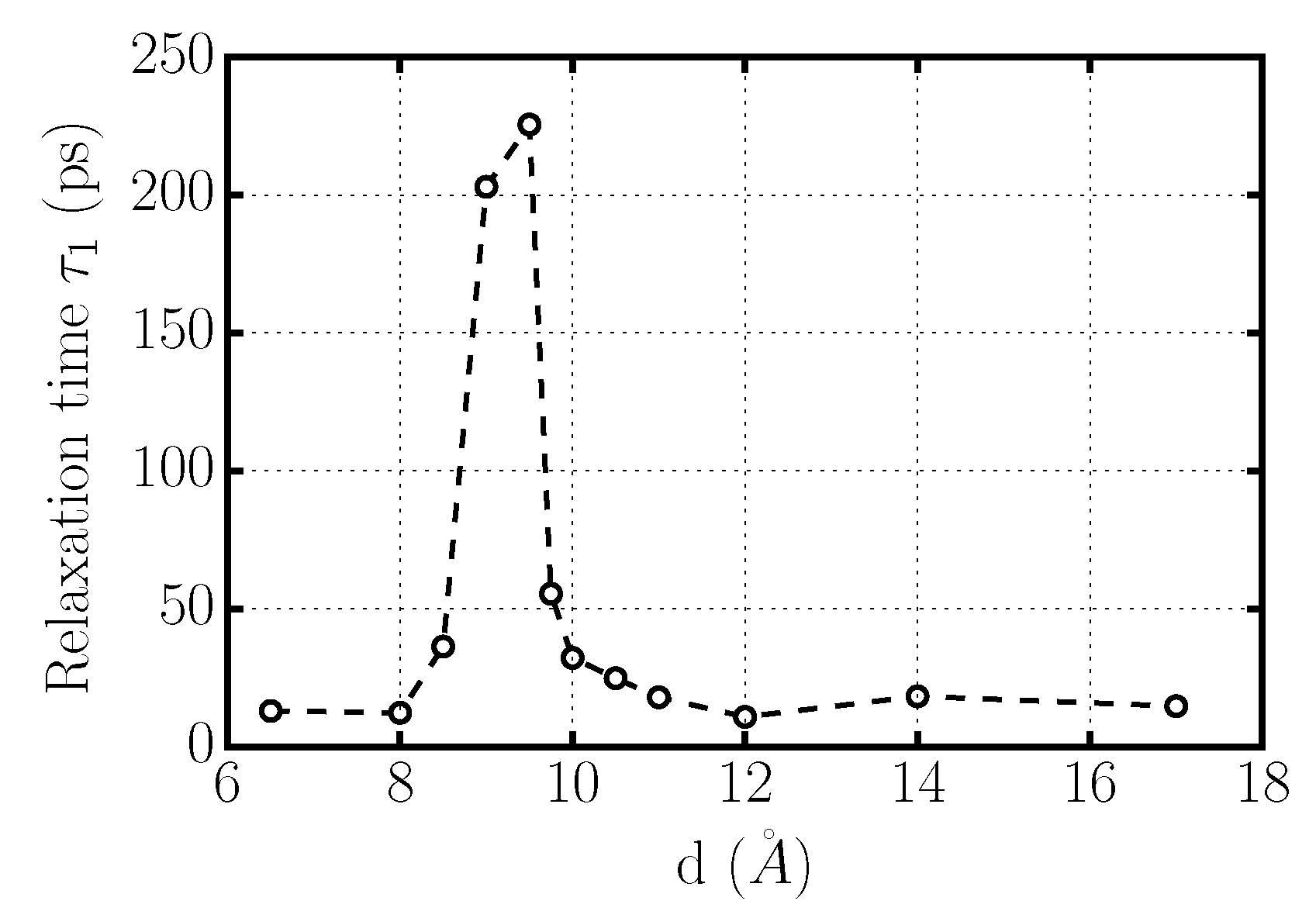
Complementary information can be reached by studying the rotational dynamics of water confined within the graphene sieve for different inter-plate separations d. To this end, we compute the rotational dipolar correlation function
where is the direction of the water dipole vector at time t and denote ensemble average over different time origins and over all water molecules confined between graphene plates separated a distance d. To quantify the relaxation of the correlation functions , we define the relaxation time
which is independent of the specific functional form of the correlation function (Figure 7). For 6.5 Å Å and Å water molecules reorient with an approximately constant typical time. The reorientation of water molecules becomes much slower for 8.5 Å Å, indicating the transition to a solid phase. This interpretation is consistent with our structural analysis, presented next.
3.2. Structure of Confined Water
To analyze the structure of the confined water and to characterize its phases under confinement, we calculate the density profiles of water between graphene sheets along the Z-direction perpendicular to the walls at different inter-plate separations d.
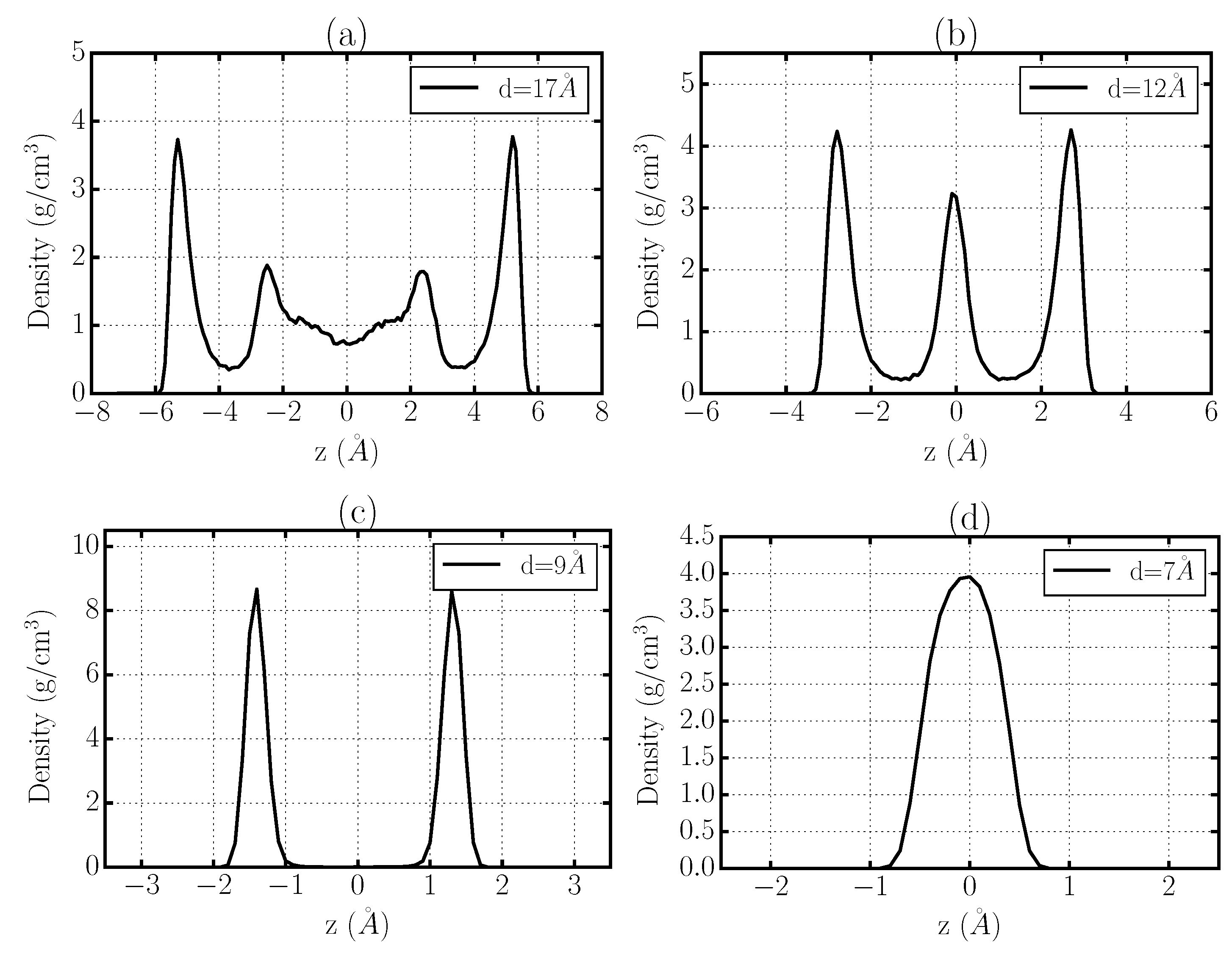
First, we observe that at the considered thermodynamic conditions bulk TIP4P/2005-water is liquid. As can be expected, in our simulations we find that for large-enough Å (Figure 8a) the system has a central bulk region between the graphene sheets and two well defined interfacial layers near each wall. By reducing d, we observe that water organizes in four layers at Å (not shown) and three layers for 11 Å Å (Figure 8b). Our analysis of its microscopical dynamics (Figure 6 and Figure 7) clearly shows that confined water remains liquid under these conditions.
For 8 Å Å (Figure 8c) we find that water forms two layers. This range of distances is where we estimate the slow-down of the dynamics (Figure 6 and Figure 7). Therefore, we careful analyze the case in which we observe the dynamical arrest, at 9 Å Å, and find that the two identical density peaks for the distribution of water are well-differentiated, with a region in between with no presence of water, and with no molecule interchange between them. Therefore, water crystallizes into a bilayer hexagonal ice phase, as can be directly checked by inspection of the snapshots (Figure 5). This crystallization is solely induced by the confinement with the sub-nm inter-plate distance and occurs within the simulated ns time-scale of our simulations spontaneously. Therefore, this range of hydrophobic confinement enhances the melting point of water of at least 25 K [89,90]. The real enhancement should be calculated by checking at which T bulk TIP4P/2005-water spontaneously crystallizes within hundreds of ns in equilibrium MD simulations.
If we reduce the inter-plate distance further, at 6.5 Å Å our data (Figure 8d) show that confined water forms a single layer and melts again. In particular, based on our analysis of microscopical dynamics (Figure 6 and Figure 7) we can conclude that water rapidly diffuses at these sub-nanometric values of d. This result could be particularly interesting in view of recent experimental attempts to filter waters with graphene-based sub-nm membranes [48].
Finally, at the smallest separation we analyze, 6 Å Å (not shown), we find that water molecules effectively deplete the confined region despite not being sterically forbidden. Therefore, for Å water evaporates under hydrophobic confinement.
To better understand the predicted reentrant crystallization by sub-nm hydrophobic confinement and the evaporation by extremely small hydrophobic confinement, we calculate as a function of d the average number of HBs per water molecule within the confined space. Here we adopted a geometric definition of HBs that is slightly less restrictive than the one defined in Section 2, with the same but with Å (instead of 3.37 Å). This difference is mainly due to the different water model considered here. We find that for confining distances Å the number of HBs per water molecule is between 3.65 and 3.7 independent on d. For confinements with 8.5 Å Å, this number becomes significantly higher, reaching a value of 3.9—very close to saturation—for Å. For Å, the number of HBs per molecule sharply decreases.
These findings allow us to rationalize the reentrant crystallization. The increase of HBs per molecule just below 1 nm confinement is consistent with the formation of a crystal structure. Indeed, the decrease in internal energy, associated with the increase of number of HBs, possibly compensates for the entropy decrease of the crystal with respect to the liquid, favoring the crystallization.
On the other hand, a further decrease of d makes geometrically impossible to create a network of highly connected water molecules. Therefore, confined water re-melts into the liquid state.
At Å the large decrease of HBs per molecules together with the huge entropy loss due to the extreme confinement makes the free energy of water between the walls too high with respect to that of free water. Therefore, the water evaporates under extreme hydrophobic confinement.
4. Computational Methods
4.1. Water Adsorbed at the Outside of Rigid CNTs and on Flat Graphene
The studies, reviewed here, of liquid water adsorbed at the external surface of armchair single-walled CNTs of the type (), with and water adsorbed in flat graphene have been performed by NVT simulations.
For each of the CNTs considered, a set of (about 10) simulations with different number of water molecules has been performed to analyze the thermodynamic stability of the water layer. Once we determined the minimum surface density of water molecules needed to uniformly cover each of the CNTs surfaces, the authors focused on the stable system with less water molecules and studied the structural and dynamical properties of the water layer. Characteristics of the selected stable systems are summarized in Table 1.
The considered simulation boxes were: 60.0 × 60.0 × 76.21 Å3 for water-(5,5)CNT system, 100.0 × 100.0 × 64.3 Å3 for the water-(9,9)CNT, 150.0 × 150.0 × 83.35 Å3 for water-(12,12)CNT, and 31.929 × 34.032 × 40 Å3 for water-graphene, with periodicity along all three spatial directions. All carbon atoms were explicitly taken into account in the calculation and were considered to be rigid, i.e., the carbon atoms were not allowed to move in the simulation runs. This approximation was investigated in detail in a previous study [78], which concluded that the mobility of carbons does not induce any noticeable change in the structure and dynamics of interfacial water. Nevertheless, a set of simulations with flexible armchair CNTs and flexible graphene have been conducted to verify the rigid-carbon approximation and to compute vibrational spectra of carbons.
Initial configurations of the different systems were produced with the help of the 1.9 version of the Visual Molecular Dynamics software [91]. All simulations were performed using the NAMD-2.7 molecular dynamics package. Water-water and water-carbon interactions have been modeled by means of the CHARMM27 force field included in the package NAMD-2.7, especially designed for the simulation of biophysical systems [92]. The interactions concerning water and carbon are a combination of Coulomb interactions (water-water) with Lennard-Jones ones (water-water, water-carbon). Water has been modeled by using the TIP3P model [74]. The Lennard-Jones parameters for the water-carbon interaction are Å, kcal/mol, Å, and kcal/mol. The long-ranged electrostatic interactions have been calculated by means of the particle mesh Ewald method [93]. The velocity Verlet algorithm has been used, together with temperature control using Langevin dynamics and a multiple time step methodology, with an integration time step of 0.5 fs for local interactions and another four times larger for long-ranged interactions. The equilibration in all cases ran for at least 100 ps, and the averages were calculated in runs of lengths longer than 1 ns.
4.2. Corrugated Graphene
The simulation set consisted of a variable number of water molecules placed on top of one graphene model sheet at room temperature (298 K). The dimensions of the simulation cell were similar to those used in a previous work on graphene [49], i.e., Å, Å, Å with periodic boundary conditions in all directions. The larger length in the Z direction allowed the authors to make sure that the influence of water images in the properties of the simulated liquid was negligible, as it will be explained below. The carbon layer could be perfectly flat or with some degree of roughness. The latter was introduced by applying a distortion in the Z direction to the positions of the carbon atoms in the graphene sheet, while the X and Y coordinates were kept constant with respect to the flat case. Two types of distortions were applied, a regular one, given by the functions:
or
and a random one, in which the positions of the carbon atoms were changed a random distance, up or down, from the ones in a flat graphene layer. The maximum distance in all cases was given by the parameter A, that indicates the amplitude of the roughness, and was taken to be 0.7 and 5 Å, according to previous accounts of the degree of roughness of graphene [94,95,96].
However, when the authors proceed in this way they were creating structures rougher than the ones observed in experiments, in the sense that the wavelength of the distortion () is smaller than the values found for corrugated structures, sometimes not by much (around 3.4 nm versus 5 nm in [95]) but others in a non neglectable way (370 nm and above in [97] in which the degree of distortion in the Z direction is also bigger from 7 Å up). The goal was to compare the results so obtained with the ones for a perfectly flat surface of the same dimensions given in [49].
Water molecules were modeled by means of a flexible SPC (simple point charge potential) [98] which is able to correctly reproduce the main features of the experimental infrared spectrum of liquid bulk water at 298 K, in particular, the location of maxima of the main spectral bands. The model was re-parameterized from an earlier version by Toukan and Rahman [99] and it has been successfully tested for water in a wide variety of thermodynamical conditions [80,100] and used for water under mechanical confinement [57]. It should be pointed out that within this model molecular dipole moments are variable and, consequently, polarizability effects due to dipole-dipole interactions are taken into account up to some degree. Water-carbon interactions have been modeled with the same potential as in previous works [70], namely a Lennard-Jones model where individual carbon-oxygen and carbon-hydrogen forces were obtained through the application of the Lorentz–Bertherlot rules. Here we should stress that presumably corrugation will create sp3/sp3-like C atoms, which would interact with water in a different manner that usual sp2 bonded C atoms would do. However, it has been shown that such different hybridizations would only affect about 5% the parameters of the Lennard-Jones potential [101]. This allows one to keep the use of the same parameters along simulation runs.
Long-range electrostatic interactions have been calculated by means of Ewald sums since, as it was demonstrated by Yeh and Berkowitz [102] and independently by Spohr [103], such procedure is fully equivalent to the Ewald procedure, which corresponds to systems with periodic boundary conditions in only two dimensions. The only requirement that should be imposed is a box length in the non-isotropic perpendicular direction to graphene (Z-axis) of at least five times the size of the water-graphene set along X and Y directions. This fact allows one to avoid the use of the computationally very expensive version.
Finally, the authors used a leap-frog Verlet integration algorithm coupled to a thermal bath [104], in order to keep the temperature of the system fluctuating within a reasonable range (around 10% of average values). The integration time step was 0.5 fs, with equilibration periods of 100 ps. Averages of dynamical quantities were computed from runs that at least 250 ps.
4.3. Water Confined between Graphene Plates
We have also analyzed the properties of water confined in between graphene sheets. To this end we simulated two fixed and rigid 24.6 Å × 25.5 Å graphene plates on top of each other immersed in 2796 water molecules, as shown schematically in Figure 5. The idea of the setup is to create a reservoir of bulk water with approximately constant pressure and chemical potential irrespective of the properties of the water confined between the graphene plates. We consider cases with fixed graphene plate separation Å (the distance d is defined from the center of carbon atoms). Periodic boundary conditions are applied along the three spatial directions.
Carbon atoms in the graphene sheets are maintained at fixed positions throughout the simulation. The parameters of the non-bonded Lennard-Jones interactions of carbon atoms are taken from the CHARMM27 force field [92]. Water molecules are described using the TIP4P/2005 model, which has been shown to reproduce well dynamical and structural properties of bulk water [87]. The Lorentz–Bertherlot rules are used to produce the parameters of the water-carbon interactions.
All simulations are performed using GROMACS simulation package [105] with a simulation time step of 2 fs. Van der Waals interactions are cut off at 14 Å with a smooth switching function starting at 10 Å. The long-range electrostatic forces are computed using the particle mesh Ewald method [93] with a grid space of Å. We update the electrostatic interactions every 2 fs. We use a Berendsen thermostat [104] with a time constant of 0.5ps to control the temperature of the simulated system.
5. Conclusions
Free energy calculations, based on MD simulations, of liquid water at ambient conditions adsorbed at the external walls of several armchair CNTs, with diameters ranging form 0.27 to 1.18 nm, and flat graphene sheets show that thermodynamically stable wetting depends on the curvature of the interface. In particular, flat graphene or CNTs with a large radius of curvature, such as (12,12), are not coated by water, while CNTs (9,9) and (5,5), with a smaller radius of curvature, are fully coated [49].
The studies of structure of water adsorbed on a series of corrugated graphene surfaces reveal differences with the former cases [78]. For large distortion amplitude (5 Å) of the surface the analysis shows a decrease of approximate 1–2% for the water-to-surface binding energy [78]. Overall, zero and small corrugation amplitudes leads to more stable wetting. These results could be particularly interesting to design men-made super-hydrophobic materials that mimics the nanostructures like mosquito eyes or cicada wings which exhibit anti-fogging and self-cleaning properties [47].
The simulations of water at the interface of flat rigid graphene or at the outside surface of CNTs show that the surface affects the nearby water structure, breaking some of the HBs and inducing two particular water arrangements: dangling hydrogens or water with molecular plane parallel to the interface. However, no significant differences arise in the translational dynamics depending on the curvature.
In addition, the study of the water dynamics at a variety of corrugated graphene interfaces does not show significant dependence on the distortion amplitude of the surface. The simulations reveal that oxygen diffusion at interfaces is slightly faster than in the bulk but independent of the corrugation. Nevertheless, a clear dependence is estimated at the water-vacuum interface in the farthest region from the carbon surface possibly due to the important reduction in the number of HBs at such interface.
Another evident dependence of the dynamics on the surface properties—specifically, the curvature—is predicted for water inside the CNTs. The translation diffusion of water decreases for decreasing CNT radius of curvature. The water longitudinal diffusion along the CNT axis is faster than that along its section and, interestingly, is not monotonous with the CNT diameter. In particular, the longitudinal diffusion decreases for CNT with diameters nm and increases when the diameter is nm. This prediction intriguingly correlates with other more recent results [57,66,67,68,69] in which the characteristic 1 nm length-scale has been discussed in relation to a change in the diffusion regime of water.
Therefore, in this work we analyze another geometry for graphene-based confinements where it is possible to tune the confining distance and test how relevant is the 1 nm length-scale for the diffusion. By doing so, we also understand the reason why this length-scale is relevant for water.
We consider a sieve made of two parallel graphene layers at a distance d. Our simulations show that at ambient conditions water diffusion slowly decreases when d reduces and that the parallel diffusion of the confined water vanishes for nm. By further reduction of d, we find that water parallel diffusion increases up to turning close to the bulk value when d approaches 0.7 nm. We find a similar behavior for the rotational dynamics of confined water.
We show that the drastic reduction of the diffusion coefficient corresponds to the structuring of water in layers parallel to the confining walls. For nm we find a central bulk region of liquid water and two well defined interfacial layers near each wall. By reducing nm we predict that water crystallizes forming two hexagonal ice layers at nm. By further reduction inter-plate distance, at nm water re-melts and, finally, for nm water evaporates within the confined region. Our analysis of the number of HBs formed by confined water, confirms our conclusions and allows us to give a rationale for the crystallization, re-melting and evaporation under confinement in terms of the total free energy of the system. Our results about structure and dynamics of confined water could be relevant for understanding potential uses of graphene-based filters for water [48].
Acknowledgments
The authors thank financial support from Spanish Ministry of Economy and Knowledge (MINECO) and the European Fund for Regional Development (FEDER) with grants FIS2015-66879-C2-1-P and FIS2015-66879-C2-2-P and from Barcelona Supercomputing Centre (projects FI-2014-1-0004, QCM-2014-1-0032 and QCM-2014-2-0032).
Author Contributions
Jordi Martí, Carles Calero and Giancarlo Franzese reviewed the relevant literature and wrote the manuscript. Carles Calero and Giancarlo Franzese planned the new simulations. Carles Calero performed the new simulations and analyzed the new data with Giancarlo Franzese. Jordi Martí and Giancarlo Franzese coordinated the work. All authors have read and approved the final manuscript.
Conflicts of Interest
The authors declare no conflict of interest.
References
- Gileadi, E.; Kirowa-Eisner, E.; Penciner, J. Interfacial Electrochemistry; Addison-Wesley: Reading, MA, USA, 1975. [Google Scholar]
- Thiel, P.A.; Madey, T.E. The interaction of water with solid surfaces: fundamental aspects. Surf. Sci. Rep. 1987, 7, 211–385. [Google Scholar] [CrossRef]
- Butler, G.; Ison, H.C.K. Corrosion and Its Prevention in Waters; Reinhold: New York, NY, USA, 1966. [Google Scholar]
- Bartón, K. Protection against Atmosferic Corrosion: Theories and Methods; Wiley: London, UK, 1976. [Google Scholar]
- Turner, J.E.; Hendewerk, M.; Somorjai, G.A. The photodissociation of water by doped iron oxides: The unbiased p/n assembly. Chem. Phys. Lett. 1984, 105, 581–585. [Google Scholar] [CrossRef]
- Xue, G.; Xu, Y.; Ding, T.; Li, J.; Yin, J.; Fei, W.; Cao, Y.; Yu, J.; Yuan, L.; Gong, L.; et al. Water-evaporation-induced electricity with nanostructured carbon materials. Nat. Nano 2017. [Google Scholar] [CrossRef] [PubMed]
- Pruppacher, H.R.; Klett, J.D. Microphysics of Clouds and Precipitation; Springer: Dordrecht, The Netherlands, 1978; pp. 257–268. [Google Scholar]
- Kim, J.; Lu, W.; Qiu, W.; Wang, L.; Caffey, M.; Zhong, D. Ultrafast hydration dynamics in the lipidic cubic phase: Discrete water structures in nanochannels. J. Phys. Chem. B 2006, 110, 21994–22000. [Google Scholar] [CrossRef] [PubMed]
- Tong, J.; Briggs, M.M.; McIntosh, T.J. Water permeability of aquaporin-4 channel depends on bilayer composition, thickness, and elasticity. Biophys. J. 2012, 103, 1899–1908. [Google Scholar] [CrossRef] [PubMed]
- Russo, C.J.; Passmore, L.A. Progress towards an optimal specimen support for electron cryomicroscopy. Curr. Opin. Struct. Biol. 2016, 37, 81–89. [Google Scholar] [CrossRef] [PubMed]
- Gelb, L.D.; Gubbins, K.E.; Radhakrishnan, R.; Sliwinska-Bartowiak, M. Phase separation in confined systems. Rep. Prog. Phys. 1999, 62, 1573–1660. [Google Scholar] [CrossRef]
- Evans, R.; Marini Bettolo Marconi, U.; Tarazona, P. Fluids in narrow pores: Adsorption, capillary condensation, and critical points. J. Chem. Phys. 1986, 84, 2376–2399. [Google Scholar] [CrossRef]
- Bal, P.C.; Evans, R. Temperature dependence of gas adsorption on a mesoporous solid: Capillary criticality and hysteresis. Langmuir 1989, 5, 714–723. [Google Scholar] [CrossRef]
- Zangi, R.; Mark, A.E. Monolayer Ice. Phys. Rev. Lett. 2003, 91, 025502. [Google Scholar] [CrossRef] [PubMed]
- Zangi, R. Water confined to a slab geometry: A review of recent computer simulation studies. J. Phys. Condens. Matter 2004, 16, S5371–S5388. [Google Scholar] [CrossRef]
- Kumar, P.; Buldyrev, S.V.; Starr, F.W.; Giovambattista, N.; Stanley, H.E. Thermodynamics, structure, and dynamics of water confined between hydrophobic plates. Phys. Rev. E 2005, 72, 051503. [Google Scholar] [CrossRef] [PubMed]
- Vilanova, O.; Franzese, G. Structural and dynamical properties of nanoconfined supercooled water. arXiv, 2011; arXiv:1102.2864. [Google Scholar]
- Chen, J.; Schusteritsch, G.; Pickard, C.J.; Salzmann, C.G.; Michaelides, A. Two Dimensional Ice from First Principles: Structures and Phase Transitions. Phys. Rev. Lett. 2016, 116, 025501. [Google Scholar] [CrossRef]
- Corsetti, F.; Matthews, P.; Artacho, E. Structural and configurational properties of nanoconfined monolayer ice from first principles. Sci. Rep. 2016, 6, 18651. [Google Scholar] [CrossRef] [PubMed]
- Lee, C.Y.; McCammon, J.A.; Rossky, P.J. The structure of liquid water at an extended hydrophobic surface. J. Chem. Phys. 1984, 80, 4448–4455. [Google Scholar] [CrossRef]
- Zhu, S.-B.; Robinson, G.W. Structure and dynamics of liquid water between plates. J. Chem. Phys. 1990, 94, 1403–1410. [Google Scholar] [CrossRef]
- Mamatkulov, S.I.; Khabibullaev, P.K.; Netz, R.R. Water at hydrophobic substrates: curvature, pressure, and temperature effects. Langmuir 2004, 20, 4756–4763. [Google Scholar] [CrossRef] [PubMed]
- Choudhury, N.; Pettitt, B.M. On the mechanism of hydrophobic association of nanoscopic solutes. J. Am. Chem. Soc. 2005, 127, 3556–3567. [Google Scholar] [CrossRef] [PubMed]
- Choudhury, N.; Pettitt, B.M. Dynamics of water trapped between hydrophobic solutes. J. Phys. Chem. B 2005, 109, 6422–6429. [Google Scholar] [CrossRef] [PubMed]
- Gallo, P.; Rovere, M. Anomalous dynamics of confined water at low hydration. J. Phys. Condens. Matter 2003, 15, 7625–7633. [Google Scholar] [CrossRef]
- Rovere, M.; Ricci, M.A.; Vellati, D.; Bruni, F. A molecular dynamics simulation of water confined in a cylindrical SiO2 pore. J. Chem. Phys. 1998, 108, 9859–9867. [Google Scholar] [CrossRef]
- Spohr, E. Computer simulation of the water/platinum interface. Dynamical results. Chem. Phys. 1990, 141, 87–94. [Google Scholar] [CrossRef]
- Rustad, J.R.; Felmy, A.R.; Bylaska, E.J. Molecular simulation of the magnetite-water interface. Geochim. Cosmochim. Acta 2003, 67, 1001–1016. [Google Scholar] [CrossRef]
- Martins, L.R.; Skaf, M.S.; Ladanyi, B.M. Solvation dynamics at the water/zirconia interface: Molecular dynamics simulations. J. Phys. Chem. B 2004, 108, 19687–19697. [Google Scholar] [CrossRef]
- Gordillo, M.C.; Martí, J. Molecular dynamics description of a layer of water molecules on a hydrophobic surface. J. Chem. Phys. 2002, 117, 3425–3430. [Google Scholar] [CrossRef]
- Striolo, A.; Chialvo, A.; Cummings, P.T.; Gubbins, K.E. Water adsorption in carbon-slit nanopores. Langmuir 2003, 19, 8583–8591. [Google Scholar] [CrossRef]
- Cabrera Sanfelix, P.; Holloway, S.; Kolasinski, K.W.; Darling, G.R. The structure of water on the (0001) surface of graphite. Surf. Sci. 2003, 532–535, 166–172. [Google Scholar] [CrossRef]
- Pertsin, A.; Grunze, M. Water-graphite interaction and behavior of water near the graphite surface. J. Phys. Chem. B 2004, 108, 1357–1364. [Google Scholar] [CrossRef]
- Gordillo, M.C.; Nagy, G.; Martí, J. Structure of water nanoconfined between hydrophobic surfaces. J. Chem. Phys. 2005, 123, 054707. [Google Scholar] [CrossRef] [PubMed]
- Hummer, G.; Rasaiah, J.C.; Noworyta, J.P. Water conduction through the hydrophobic channel of a carbon nanotube. Nature 2001, 414, 188–190. [Google Scholar] [CrossRef] [PubMed]
- Gordillo, M.C.; Martí, J. Water on the outside of carbon nanotube bundles. Phys. Rev. B. 2003, 67, 205425. [Google Scholar] [CrossRef]
- Striolo, A.; Chialvo, A.; Cummings, P.T.; Gubbins, K.E. Simulated water adsorption in chemically heterogeneous carbon nanotubes. J. Chem. Phys. 2006, 124, 074710. [Google Scholar] [CrossRef] [PubMed]
- Nagy, G. Water structure at the graphite (0001) surface by STM measurements. J. Electroanal. Chem. 1996, 409, 19–23. [Google Scholar] [CrossRef]
- Daio, T.; Bayer, T.; Ikuta, T.; Nishiyama, T.; Takahashi, K.; Takata, Y.; Sasaki, K.; Matthew Lyth, S. In-Situ ESEM and EELS Observation of Water Uptake and Ice Formation in Multilayer Graphene Oxide. Sci. Rep. 2015, 5, 11807. [Google Scholar] [CrossRef] [PubMed]
- Scodinu, A.; Fourkas, J.T. Comparison of the orientational dynamics of water confined in hydrophobic and hydrophilic nanopores. J. Phys. Chem. B 2002, 106, 10292–10295. [Google Scholar] [CrossRef]
- Teschke, O.; de Souza, E.F. Water molecular arrangement at air/water interfaces probed by atomic force microscopy. Chem. Phys. Lett. 2005, 403, 95–101. [Google Scholar] [CrossRef]
- Tombari, E.; Salvetti, G.; Ferrari, C.; Johari, G.P. Thermodynamic functions of water and ice confined to 2 nm radius pores. J. Chem. Phys. 2005, 122, 104712. [Google Scholar] [CrossRef] [PubMed]
- Ricci, M.A.; Bruni, F.; Gallo, P.; Rovere, M.; Soper, A.K. Water in confined geometries: experiments and simulations. J. Phys. Condens. Matter 2000, 12, A345–A350. [Google Scholar] [CrossRef]
- Janiak, C.; Scharmann, T.G.; Mason, S.A. Two-dimensional water and ice layers: Neutron diffraction studies at 278, 263, and 20 K. J. Am. Chem. Soc. 2002, 124, 14010–14011. [Google Scholar] [CrossRef] [PubMed]
- Kolesnikov, A.I.; Zanotti, J.-M.; Loong, C.-K.; Thiyagarajan, P.; Moravsky, A.P.; Loufty, R.O.; Burnham, C.J. Anomalously soft dynamics of water in a nanotube: a revelation of nanoscale confinement. Phys. Rev. Lett. 2004, 93, 035503. [Google Scholar] [CrossRef] [PubMed]
- Sliwinska-Bartkoviak, M.; Jazdzewska, M.; Huan, L.L.; Gubbins, K.E. Melting behavior of water in cylindrical pores: Carbon nanotubes and silica glasses. Phys. Chem. Chem. Phys. 2008, 10, 4909–4919. [Google Scholar] [CrossRef] [PubMed]
- Mouterde, T.; Lehoucq, G.; Xavier, S.; Checco, A.; Black, C.T.; Rahman, A.; Midavaine, T.; Clanet, C.; Quere, D. Antifogging abilities of model nanotextures. Nat. Mater. 2017. [Google Scholar] [CrossRef] [PubMed]
- Abraham, J.; Vasu, K.S.; Williams, C.D.; Gopinadhan, K.; Su, Y.; Cherian, C.; Dix, J.; Prestat, E.; Haigh, S.J.; Grigorieva, I.V.; et al. Tuneable Sieving of Ions Using Graphene Oxide Membranes. arXiv, 2017; arXiv:1701.05519. [Google Scholar]
- Gordillo, M.C.; Martí, J. Structure of water adsorbed on a single graphene sheet. Phys. Rev. B. 2008, 78, 075432. [Google Scholar] [CrossRef]
- Iijima, S. Helical microtubules of graphitic carbon. Nature 1991, 354, 56–58. [Google Scholar] [CrossRef]
- Saito, R.; Dresselhaus, G.; Dresselhaus, M.S. Physical Properties of Carbon Nanotubes; Imperial College Press: London, UK, 1998. [Google Scholar]
- Calero, C.; Gordillo, M.C.; Martí, J. Size effects on water adsorbed on hydrophobic probes at the nanometric scale. J. Chem. Phys. 2013, 138, 214702. [Google Scholar] [CrossRef] [PubMed] [Green Version]
- Werder, T.; Walther, J.H.; Jaffe, R.L.; Halicioglu, T.; Koumoutsakos, P. On the water-carbon interaction for use in molecular dynamics simulations of graphite and carbon nanotubes. J. Phys. Chem. B 2003, 107, 1345–1352. [Google Scholar] [CrossRef]
- Martí, J. Dynamic properties of hydrogen-bonded networks in supercritical water. Phys. Rev. E 2000, 61, 449–456. [Google Scholar] [CrossRef]
- Boero, M.; Terakura, K.; Ikeshoji, T.; Liew, C.C.; Parrinello, M. Hydrogen bonding and dipole moment of water at supercritical conditions: A first-principles molecular dynamics study. Phys. Rev. Lett. 2000, 85, 3245–3248. [Google Scholar] [CrossRef] [PubMed]
- Matubayasi, N.; Wakai, C.; Nakahara, M. Structural study of supercritical water. I. Nuclear magnetic resonance spectroscopy. J. Chem. Phys. 1997, 107, 9133–9140. [Google Scholar] [CrossRef]
- Martí, J.; Nagy, G.; Gordillo, M.C.; Guàrdia, E. Molecular simulation of liquid water confined inside graphite channels: Thermodynamics and structural properties. J. Chem. Phys. 2006, 124, 094703. [Google Scholar] [CrossRef] [PubMed]
- Nagy, G.; Gordillo, M.C.; Guàrdia, E.; Martí, J. Liquid water confined in carbon nanochannels at high temperatures. J. Phys. Chem. B 2007, 111, 12524–12530. [Google Scholar] [CrossRef] [PubMed]
- Cicero, G.; Grossman, J.K.; Schwegler, E.; Gygi, F.; Galli, G. Water confined in nanotubes and between graphene sheets: A first principle study. J. Am. Chem. Soc. 2008, 130, 1871–1878. [Google Scholar] [CrossRef] [PubMed]
- Choudhury, N. On the Manifestation of Hydrophobicity at the Nanoscale. J. Phys. Chem. B 2008, 112, 6296–6300. [Google Scholar] [CrossRef] [PubMed]
- Madden, P.; Kivelson, D. A consistent molecular treatment of dielectric phenomena. Adv. Chem. Phys. 1984, 56, 467–566. [Google Scholar]
- Gilijamse, J.J.; Lock, A.J.; Bakker, H.J. Dynamics of confined water molecules. Proc. Natl. Acad. Sci. USA 2005, 102, 3202–3207. [Google Scholar] [CrossRef] [PubMed]
- Tummala, N.R.; Striolo, A. Hydrogen-Bond Dynamics for Water Confined in Carbon Tetrachloride-Acetone Mixtures. J. Phys. Chem. B 2008, 112, 10675–10683. [Google Scholar] [CrossRef] [PubMed]
- Martí, J.; Nagy, G.; Gordillo, M.C.; Guàrdia, E. Molecular dynamics simulation of liquid water confined inside graphite channels: Dielectric and dynamical properties. J. Phys. Chem. B 2006, 110, 23987–23994. [Google Scholar] [CrossRef] [PubMed]
- Martí, J.; Gordillo, M.C. Temperature effects on the static and dynamic properties of liquid water inside nanotubes. Phys. Rev. E 2001, 64, 021504. [Google Scholar] [CrossRef] [PubMed]
- Ye, H.; Zhang, H.; Zheng, Y.; Zhang, Z. Nanoconfinement induced anomalous water diffusion inside carbon nanotubes. Microfluid. Nanofluid. 2011, 10, 1359–1364. [Google Scholar] [CrossRef]
- Zheng, Y.-G.; Ye, H.-F.; Zhang, Z.-Q.; Zhang, H.-W. Water diffusion inside carbon nanotubes: Mutual effects of surface and confinement. Phys. Chem. Chem. Phys. 2012, 14, 964–971. [Google Scholar] [CrossRef] [PubMed]
- Bordin, J.R.; de Oliveira, A.B.; Diehl, A.; Barbosa, M.C. Diffusion enhancement in core-softened fluid confined in nanotubes. J. Chem. Phys. 2012, 137, 084504. [Google Scholar] [CrossRef] [PubMed]
- de los Santos, F.; Franzese, G. Relations between the diffusion anomaly and cooperative rearranging regions in a hydrophobically nanoconfined water monolayer. Phys. Rev. E 2012, 85, 010602. [Google Scholar] [CrossRef] [PubMed]
- Gordillo, M.C.; Martí, J. Hydrogen bond structure of liquid water confined in nanotubes. Chem. Phys. Lett. 2000, 329, 341–345. [Google Scholar] [CrossRef]
- Holt, J.K.; Park, H.G.; Wang, Y.; Stadermann, M.; Artyukhin, A.B.; Grigoropoulos, C.P.; Noy, A.; Bakajin, O. Fast Mass Transport Through Sub-2-Nanometer Carbon Nanotubes. Science 2006, 312, 1034–1037. [Google Scholar] [CrossRef] [PubMed]
- Martí, J.; Gordillo, M.C. Time-dependent properties of liquid water isotopes adsorbed in carbon nanotubes. J. Chem. Phys. 2001, 114, 10486–10492. [Google Scholar] [CrossRef]
- Krynicki, K.; Green, C.D.; Sawyer, D.W. Pressure and temperature dependence of self-diffusion in water. Faraday Discuss. Chem. Soc. 1978, 66, 199–208. [Google Scholar] [CrossRef]
- Jorgensen, W.L.; Chandrasekhar, J.; Madura, J.D.; Impey, R.W.; Klein, M.L. Comparison of simple potential functions for simulating liquid water. J. Chem. Phys. 1983, 79, 926–935. [Google Scholar] [CrossRef]
- Hausser, R.; Maier, G.; Noack, F. Kernmagnetische messungen von selbstdiffusions-koeffizienten in wasser und benzol bis zum kritischen punkt. Z. Naturforsch. A 1966, 21, 1410–1415. [Google Scholar] [CrossRef]
- Martí, J.; Gordillo, M.C. Structure and dynamics of liquid water adsorbed on the external walls of carbon nanotubes. J. Chem. Phys. 2003, 119, 12540–12546. [Google Scholar] [CrossRef]
- Martí, J.; Sala, J.; Guàrdia, E. Molecular dynamics simulations of water confined in graphene nanochannels: From ambient to supercritical environments. J. Mol. Liq. 2009, 153, 72–78. [Google Scholar] [CrossRef]
- Gordillo, M.C.; Martí, J. Effect of surface roughness on the static and dynamic properties of water adsorbed on graphene. J. Phys. Chem. B 2010, 114, 4583–4589. [Google Scholar] [CrossRef] [PubMed]
- Liu, P.; Harder, E.; Berne, B.J. On the calculation of diffusion coefficients in confined fluids and interfaces with an application to the liquid-vapor interface of water. J. Phys. Chem. B 2004, 108, 6595–6602. [Google Scholar] [CrossRef]
- Martí, J.; Guàrdia, E.; Padró, J.A. Dielectric properties and infrared spectra of liquid water: Influence of the dynamic cross correlations. J. Chem. Phys. 1994, 101, 10883–10891. [Google Scholar] [CrossRef]
- Martí, J.; Padró, J.A.; Guàrdia, E. Molecular dynamics simulation of liquid water along the coexistence curve: Hydrogen bonds and vibrational spectra. J. Chem. Phys. 1996, 105, 639–649. [Google Scholar] [CrossRef]
- Algara-Siller, G.; Lehtinen, O.; Wang, F.C.; Nair, R.R.; Kaiser, U.; Wu, H.A.; Geim, A.K.; Grigorieva, I.V. Square ice in graphene nanocapillaries. Nature 2015, 519, 443–445. [Google Scholar] [CrossRef] [PubMed]
- Zangi, R.; Mark, E.A. Bilayer ice and alternate liquid phases of confined water. J. Chem. Phys. 2003, 119, 1694–1700. [Google Scholar] [CrossRef]
- Giovambattista, N.; Rossky, P.J.; Debenedetti, P.G. Phase transitions induced by nanoconfinement in liquid water. Phys. Rev. Lett. 2009, 102, 050603. [Google Scholar] [CrossRef] [PubMed]
- Han, S.; Choi, M.Y.; Kumar, P.; Stanley, H.E. Phase transitions in confined water nanofilms. Nat. Phys. 2010, 6, 685–689. [Google Scholar] [CrossRef]
- Giovambattista, N.; Rossky, P.J.; Debenedetti, P.G. Effect of pressure on the phase behavior and structure of water confined between nanoscale hydrophobic and hydrophilic plates. Phys. Rev. E 2006, 73, 041604. [Google Scholar] [CrossRef] [PubMed]
- Abascal, J.L.F.; Vega, C. A general purpose model for the condensed phases of water: TIP4P/2005. J. Chem. Phys. 2005, 123, 234505. [Google Scholar] [CrossRef] [PubMed]
- Rozmanov, D.; Kusalik, P.G. Transport coefficients in the TIP4P-2005 water model. J. Chem. Phys. 2012, 136, 044507. [Google Scholar] [CrossRef] [PubMed]
- Vega, C.; Abascal, J.L.F. Relation between the melting temperature and the temperature of maximum density for the most common models of water. J. Chem. Phys. 2005, 123, 144504. [Google Scholar] [CrossRef] [PubMed]
- Agarwal, M.; Alam, M.P.; Chakravarty, C. Thermodynamic, Diffusional, and Structural Anomalies in Rigid-Body Water Models. J. Phys. Chem. B 2011, 115, 6935–6945. [Google Scholar] [CrossRef] [PubMed]
- Humphrey, W.; Dalke, A.; Schulten, K. VMD: Visual molecular dynamics. J. Mol. Gr. 1996, 14, 33–38. [Google Scholar] [CrossRef]
- Phillips, J.C.; Braun, R.; Wang, W.; Gumbart, J.; Tajkhorshid, E.; Villa, E.; Chipot, C.; Skeel, R.D.; Kale, L.; Schulten, K. Scalable molecular dynamics with NAMD. J. Comp. Chem. 2005, 26, 1781–1802. [Google Scholar] [CrossRef] [PubMed]
- Darden, T.; York, D.; Pedersen, L. Particle mesh Ewald: An N · log (N) method for Ewald sums in large systems. J. Chem. Phys. 1993, 98, 10089–10092. [Google Scholar] [CrossRef]
- Fasolino, A.; Los, J.H.; Katsnelson, M.I. Intrinsic ripples in graphene. Nat. Mat. 2006, 6, 858–861. [Google Scholar] [CrossRef] [PubMed] [Green Version]
- Meyer, J.C.; Geim, A.K.; Katsnelson, M.I.; Novoselov, K.S.; Booth, T.J.; Roth, S. The structure of suspended graphene sheets. Nature 2007, 446, 60–63. [Google Scholar] [CrossRef] [PubMed] [Green Version]
- Abedpour, N.; Neek-Amal, M.; Asgari, R.; Shahbazi, F.; Nafari, N.; Tabar, M.R.R. Roughness of undoped graphene and its short-range induced gauge field. Phys. Rev. B 2007, 76, 195407. [Google Scholar] [CrossRef]
- Bao, W.; Miao, F.; Chen, Z.; Zhang, H.; Jang, W.; Dames, C.; Lau, C.N. Controlled ripple texturing of suspended graphene and ultrathin graphite membranes. Nat. Nanotechnol. 2009, 4, 562–566. [Google Scholar] [CrossRef] [PubMed]
- Martí, J.; Padró, J.A.; Guàrdia, E. Molecular dynamics calculation of the infrared spectra in liquid H2O-D2O mixtures. J. Mol. Liq. 1994, 62, 17–31. [Google Scholar] [CrossRef]
- Toukan, K.; Rahman, A. Molecular-dynamics study of atomic motions in water. Phys. Rev. B 1985, 31, 2643–2648. [Google Scholar] [CrossRef]
- Martí, J. Analysis of the hydrogen bonding and vibrational spectra of supercritical model water by molecular dynamics simulations. J. Chem. Phys. 1999, 110, 6876–6886. [Google Scholar] [CrossRef] [Green Version]
- Kostov, M.K.; Cheng, H.; Cooper, A.C.; Pez, G.P. Influence of carbon curvature on molecular adsorptions in carbon-based materials: A force field approach. Phys. Rev. Lett. 2002, 89, 146105. [Google Scholar] [CrossRef] [PubMed]
- Berkowitz, M.L. Ewald summation for systems with slab geometry. J. Chem. Phys. 1999, 111, 3155–3162. [Google Scholar]
- Spohr, E. Effect of electrostatic boundary conditions and system size on the interfacial properties of water and aqueous solutions. J. Chem. Phys. 1997, 107, 6342–6348. [Google Scholar] [CrossRef]
- Berendsen, H.J.C.; Postma, J.P.M.; van Gunsteren, W.F.; DiNola, A.; Haak, J.R. Molecular dynamics with coupling to an external bath. J. Chem. Phys. 1984, 81, 3684–3690. [Google Scholar] [CrossRef]
- Berendsen, H.J.C.; van der Spoel, D.; van Drunen, R. GROMACS: A message-passing parallel molecular dynamics implementation. Comput. Phys. Commun. 1995, 91, 43–56. [Google Scholar] [CrossRef]
Figure 1.
Water energy density E versus the surface density ρ for three of the four systems considered in this work, the (5,5) and (9,9) CNTs and the graphene sheet. In each panel we show simulation results (squares) and least squares fits to Equation (2) (lines) for K (a), K (b) and K (c).
Figure 1.
Water energy density E versus the surface density ρ for three of the four systems considered in this work, the (5,5) and (9,9) CNTs and the graphene sheet. In each panel we show simulation results (squares) and least squares fits to Equation (2) (lines) for K (a), K (b) and K (c).
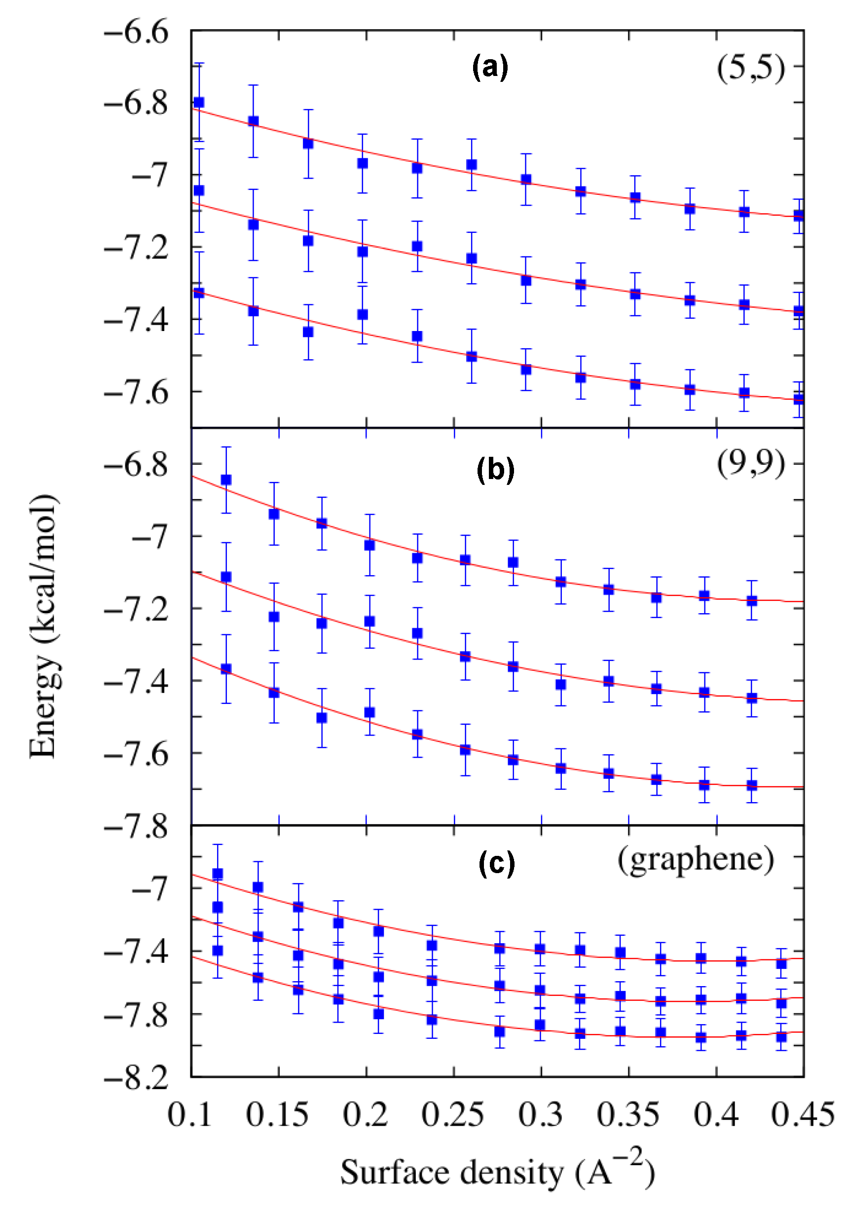
Figure 2.
Water free energy density F versus the surface per molecule for the (5,5), (9,9) and (12,12) CNTs and the graphene sheet at K, as estimated from Equations (1) and (2) using the fitting parameters calculated in Figure 1. For the thinner (5,5), (9,9) CNTs the free energy minimum is around 4.05 Å2, while for the (12,12) CNT and the graphene sheet there are no stable minima within the range of densities considered in this work.

Figure 3.
Number of HBs (lines with symbols, scale on the left) and radial oxygen density profiles (lines without symbols, scale on the right) of water adsorbed at the external volume of CNTs as a function of radial distance from the CNTs axis. The number of hydration HBs is normalized with the bulk HB number. Calculations represented with squares or dashed lines, circles or continuous lines, triangles or dotted lines are for (5,5), (9,9), (12,12) CNTs, respectively.

Figure 4.
Orientational order of water outside the CNTs as a function of the distance r from the CNTs surface. The two first Legendre polynomial (a) and (b) characterize water dipolar orientations, being the angle between the instantaneous dipole moment of water and the direction normal to the CNT surface. Symbols and lines are as in Figure 3.
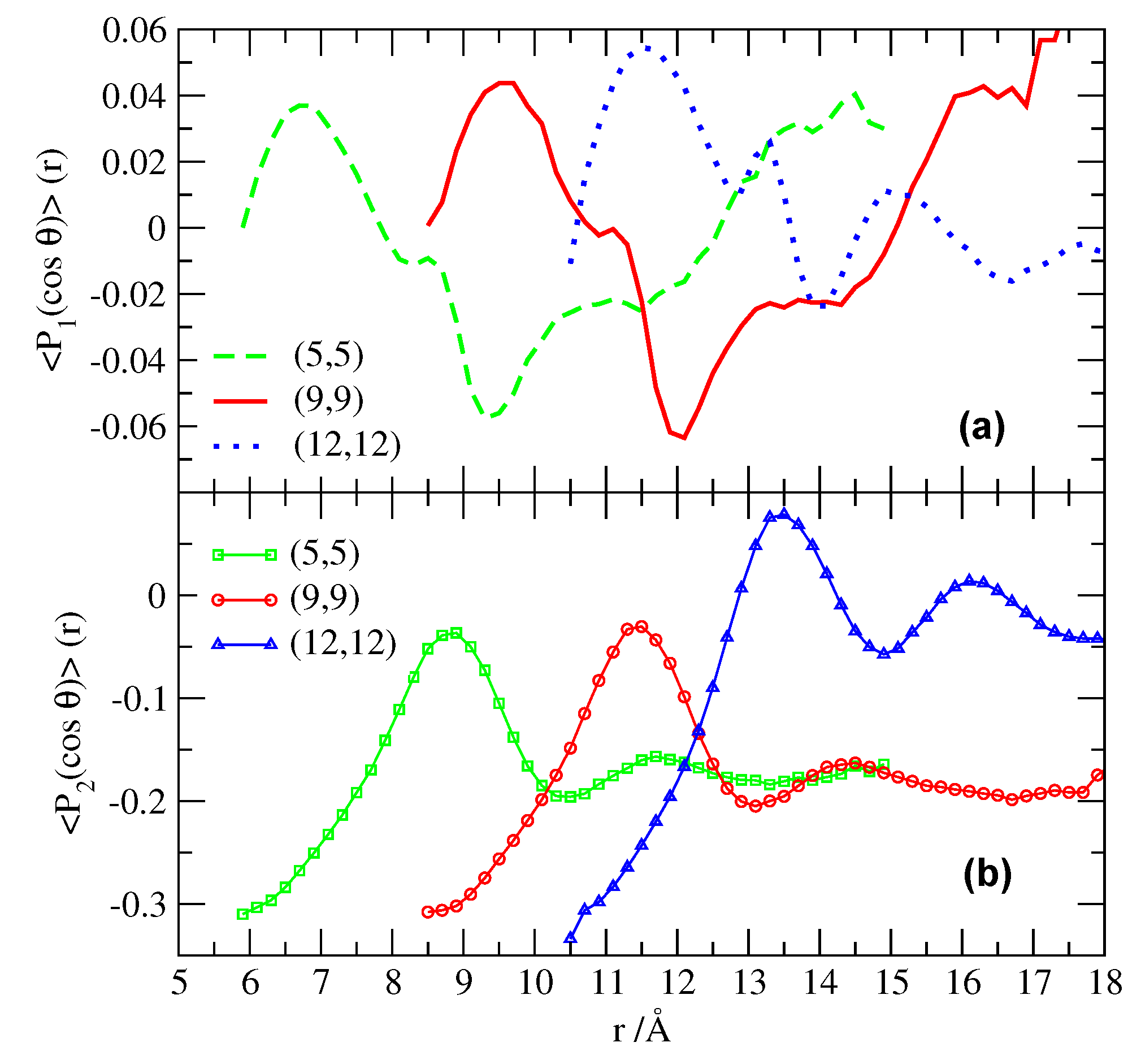
Figure 5.
Snapshot of MD simulation at K and bar of two fixed parallel graphene plates separated by Å and immersed in TIP4P/2005-water (top view). Carbon atoms are in cyan, oxygen in red, hydrogen in white. In our simulations the total number of water molecules, including those outside the confined region, remains constant while the amount of water confined between the graphene sheets depends on the spacing d. Under these conditions the confined water forms a hexagonal ice bilayer.
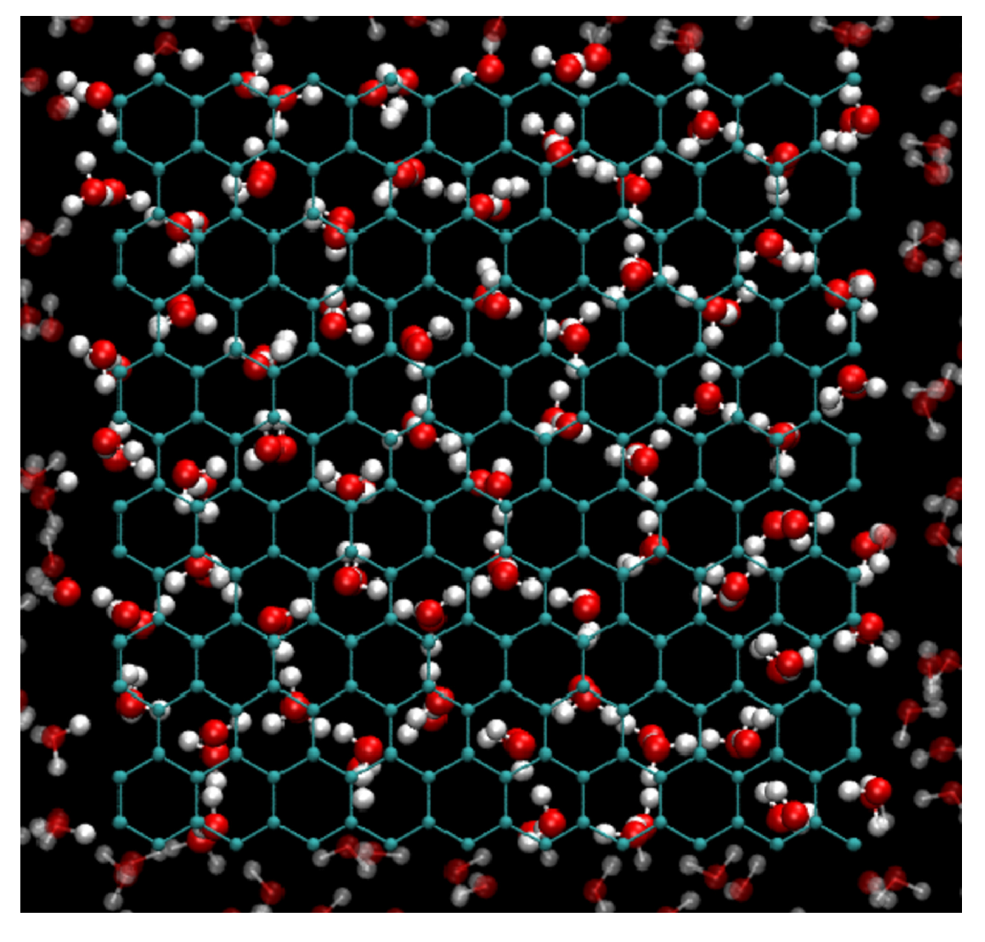
Figure 6.
Diffusion coefficient of confined TIP4P/2005-water at K and bar in a plane parallel to the graphene sheets as a function of inter-plate distance d. The dashed line is a guide to the eyes at nm2/ns, a value close to the bulk diffusion coefficient for this water model under these conditions. vanishes for 8.5 Å Å.
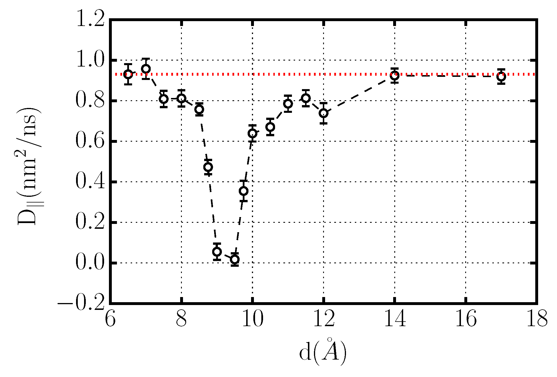
Figure 7.
Rotational relaxation time for confined TIP4P/2005-water at K and bar as a function of graphene inter-plate distance d. A large increase of , corresponding to a large slowing-down of the rotational dynamics, occurs for 8.5 Å Å.
Figure 7.
Rotational relaxation time for confined TIP4P/2005-water at K and bar as a function of graphene inter-plate distance d. A large increase of , corresponding to a large slowing-down of the rotational dynamics, occurs for 8.5 Å Å.

Figure 8.
Density profiles of TIP4P/2005-water at K and bar confined between graphene sheets along the Z-direction perpendicular to the walls at selected inter-plate separations. The occurrence of zeros between the maxima is an evidence of water layering. (a) Two interfacial layers with intermediate liquid water for graphene plates separation Å; (b) two interfacial layers with a slight-deformed intermediate layer for Å; (c) two layers for Å; (d) one layer for Å.


Table 1.
Summary of CNTs used as confining devices in our simulations. We report CNT length (l), CNT diameter (D) and number of water molecules (Nw) considered to set the density of 1 g/cm3 inside the CNT. In the case of graphene, we report the X-Y lengths.
| System | l (nm) | D (nm) | Nw |
|---|---|---|---|
| (5,5) CNT | 7.62 (Z-axis) | 0.66 | 835 |
| (9,9) CNT | 6.43 (Z-axis) | 1.22 | 935 |
| (12,12) CNT | 8.33 (Z-axis) | 1.63 | 4500 |
| Graphene | 3.19 × 3.40 | - | 1252 |
| Bulk water | - | - | 1000 |
Table 2.
Self-diffusion coefficients of water inside CNTs at room temperature from MD results for simulations with the potential model described in [72]. All values are given in 10−5 cm2/s. The experimental value has been taken from [73] for bulk liquid H2O. , and are the coefficients for overall diffusion, along the CNT axis and within a section of the CNT.
| CNT (n,m) | Dtotal | Dz−axis | Dxy−plane |
|---|---|---|---|
| (6,6) | 2.5 | 4.3 | 1.6 |
| (8,8) | 3.2 | 3.5 | 3.0 |
| (10,10) | 3.1 | 3.8 | 2.7 |
| H2O (bulk) | 2.6 | - | - |
| Experimental | 2.3 | - | - |
Table 3.
Self-diffusion coefficients along the axial direction of water outside CNTs at room temperature from MD results for simulations with the TIP3P water model [74]. All values are given in 10−5 cm2/s.
| CNT (n,m) | Dz |
|---|---|
| (5,5) | 4.9 |
| (9,9) | 4.9 |
| (12,12) | 4.6 |
| Graphene | 4.6 |
| Bulk unconstrained | 5.8 |
Table 4.
Self-diffusion coefficients of oxygen atoms near corrugated graphene. Water molecules are (i) at the graphene interface if their distance from the closest carbon is < 5 Å; (ii) in the bulk if the distance is > 7 Å and < 12 Å; (iii) at the water-vacuum interface if the distance is > 12 Å. Diffusion coefficients are expressed in 10−5 cm2/s.
| Distortion Amplitude (Å) | Type of Distortion | Water-Graphene | Bulk Region | Water-Vacuum |
|---|---|---|---|---|
| 0 | None | 3.3 | 3.1 | 3.6 |
| 0.7 | Random | 2.8 | 2.1 | 3.2 |
| 0.7 | Equation (8) | 2.8 | 2.3 | 3.7 |
| 0.7 | Equation (9) | 2.8 | 2.1 | 3.6 |
| 0.7 | Equation (7) | 2.6 | 2.2 | 3.3 |
| 5 | Equation (8) | 2.6 | 2.2 | 4.3 |
| 5 | Equation (9) | 2.6 | 2.2 | 4.2 |
| 5 | Equation (7) | 2.6 | 2.2 | 4.5 |
© 2017 by the authors. Licensee MDPI, Basel, Switzerland. This article is an open access article distributed under the terms and conditions of the Creative Commons Attribution (CC BY) license ( http://creativecommons.org/licenses/by/4.0/).
Share and Cite
MDPI and ACS Style
Martí, J.; Calero, C.; Franzese, G. Structure and Dynamics of Water at Carbon-Based Interfaces. Entropy 2017, 19, 135. https://doi.org/10.3390/e19030135
AMA Style
Martí J, Calero C, Franzese G. Structure and Dynamics of Water at Carbon-Based Interfaces. Entropy. 2017; 19(3):135. https://doi.org/10.3390/e19030135
Chicago/Turabian StyleMartí, Jordi, Carles Calero, and Giancarlo Franzese. 2017. "Structure and Dynamics of Water at Carbon-Based Interfaces" Entropy 19, no. 3: 135. https://doi.org/10.3390/e19030135
Note that from the first issue of 2016, this journal uses article numbers instead of page numbers. See further details here.