Permutation Entropy: New Ideas and Challenges

Abstract

Over recent years, some new variants of Permutation entropy have been introduced and applied to EEG analysis, including a conditional variant and variants using some additional metric information or being based on entropies that are different from the Shannon entropy. In some situations, it is not completely clear what kind of information the new measures and their algorithmic implementations provide. We discuss the new developments and illustrate them for EEG data.

1. Introduction

The concept of Permutation entropy introduced by Bandt and Pompe [1] in 2002 has been applied to data analysis in various disciplines (compare e.g., the collection [2], and papers [3,4]). The Permutation entropy of a time series is the Shannon entropy of the distribution of ordinal patterns in the time series (see also [5]). Such ordinal patterns, describing order types of vectors, are coded by permutations. Denoting the set of permutations of $\{0,1,\dots ,d\}$ for d in the natural numbers $\mathbb{N}$ by ${\mathrm{\Pi }}_d$, we say that a vector $(v_0,v_1,\dots ,v_d)\in {\mathbb{R}}^{d+1}$ has ordinal pattern $\pi =(r_0,r_1,\dots ,r_d)\in {\mathrm{\Pi }}_d$ if

$$\begin{array}{c}\hfill v_{r_0}\ge v_{r_1}\dots \ge v_{r_{d-1}}\ge v_{r_d}\end{array}$$

and

$$\begin{array}{c}\hfill r_{l-1}>r_l\mathrm{if}{v}_{r_{l-1}}=v_{r_l}.\end{array}$$

Definition 1.

The empirical Permutation entropy (ePE) of order $d\in \mathbb{N}$ and of delay $\tau \in \mathbb{N}$ of a time series ${(x_t)}_{t=0}^{N-1}$ with $N\in \mathbb{N}$ is given by

$$\begin{array}{cc}\hfill \mathrm{ePE}\left(d,\tau ,{(x_t)}_{t=0}^{N-1}\right)& =-\frac{1}{d}\sum _{\pi \in {\mathrm{\Pi }}_d}{p}_{\pi }^{\tau }ln{p}_{\pi }^{\tau },\hfill \end{array}$$

(1)

where

$$\begin{array}{cc}\hfill p_{\pi }^{\tau }& =\frac{\#\{t\in \{d\tau ,d\tau +1,\dots ,N-1\}\mid (x_t,x_{t-\tau },\dots ,x_{t-d\tau })hasordinalpattern\pi \}}{N-d\tau }\hfill \end{array}$$

(2)

is the relative frequency of ordinal patterns π in the time series and $0ln0$ is defined by 0 (compare [6]). The vectors $(x_t,x_{t-\tau },\dots ,x_{t-d\tau })$ related to $t,d$ and τ are called delay vectors.

In contrast to some other presentations of Permutation entropy in the literature, the Shannon entropy obtained from the ordinal pattern distribution is normalized by dividing by d. This is justified by an interesting statement made by Bandt et al. [7], which roughly states that for time series from a special class of systems, for $\tau =1$ and $d\to \infty$, (1) approaches a non-negative real number, however, how large the corresponding class is remains open to debate. Normalizing as given allows comparing Permutation entropy for different orders. (Some further discussion on this point follows in this paper.) Another usual normalization is given by dividing the Shannon entropy by its maximal possible value $ln(d!)$.

In order to be more flexible in data analysis, various modifications of Permutation entropy have been developed during the last years. One class of such modifications is based on adding some metric information of the corresponding delay vectors to the ordinal patterns derived. Entropy measures of that type are the fine-grained Permutation entropy proposed by Liu and Wang [8], the weighted Permutation entropy and the robust Permutation entropy introduced by Fadlallah et al. [9] and Keller et al. [10], respectively. Bian et al. [11] have adapted Permutation entropy to the situation of delay vectors with equal components which are relevant when the number of possible values in a time series is small. Other variants to consider are Tsallis or Renyi entropies instead of the Shannon entropy which goes back to the work of Zunino et al. [12] and Liang et al. [13], or to integrate information from different scales. The latter was done by Li et al. [14], Ouyang et al. [15] and Azami and Ascodero [16] on the base of averaging the original data on different scales and by Zunino et al. [17] and Zunino and Ribeiro [18]) by considering a whole spectrum of delays τ.

Unakafov and Keller [19] have proposed the Conditional entropy of (successive) ordinal patterns, which has been shown to perform better than the Permutation entropy itself in many cases.

In this paper, we discuss some of the new (“non-weighting”) developments in Permutation entropy. We first give some theoretical background in order to justify and to motivate conditional variants of Permutation entropy. Then we take a closer look at Renyi and Tsallis modifications of Permutation entropy. The last part of the paper is aimed at the classification of electroencephalography (EEG) data from the viewpoint of epileptic activity. Here, we point out that ordinal time series analysis combined with other methods and automatic learning could be promising for data analysis. We rely on EEG data reported in [6,20] and use algorithms developed in Unakafova and Keller [21].

2. Some Theoretical Background

2.1. The Kolmogorov–Sinai Entropy

In order to achieve a better understanding of Permutation entropy, we take a modeling approach. For this, we choose a discrete dynamical system defined on a probability space $(\mathrm{\Omega },\mathcal{B},P)$. The elements $\omega \in \mathrm{\Omega }$ are considered as the (hidden) states of the system, the elements of the σ-algebra $\mathcal{B}$ as the events one is interested in, and the probability P measures the chances of such events taking place. The dynamics of the system are given by a map $T:\mathrm{\Omega }\hookleftarrow$ being $\mathcal{B}-\mathcal{B}$-measurable, i.e., satisfying $T^{-1}(B)\in \mathcal{B}$ for all $B\in \mathcal{B}$. The map T is assumed to be P-invariant saying that $P(T^{-1}(A))=P(A)$ for all $B\in \mathcal{B}$, in order to guarantee that the distribution of the states of the system does not change under the dynamics.

For simplicity, during the whole paper, we assume that $(\mathrm{\Omega },\mathcal{B},P)$ and T are fixed; specifications are given directly where they are needed.

In dynamical systems, the Kolmogorov–Sinai entropy based on entropy rates of finite partitions is a well established theoretical complexity measure. For explaining this concept, consider a finite partition $\mathcal{C}=\{C_1,C_2,\dots ,C_l\}\subset \mathcal{B}$ and note that the (Shannon) entropy of such a partition is defined by

$$\begin{array}{c}\hfill H(\mathcal{C})=-\sum _{i=1}^{l}P(C_i)lnP(C_i).\end{array}$$

For $A=\{1,2,\dots ,l\}$, the set $A^k$ of words $a_1{a}_2\dots a_k$ of length k over A provides a partition ${\mathcal{C}}_k$ of Ω into pieces

$$C_{a_1{a}_2\dots a_k}:=\{\omega \in \mathrm{\Omega }|(\omega ,T(\omega ),\dots ,T^{\circ k-1}(\omega ))\in C_{a_1}\times C_{a_2}\times \dots \times C_{a_k}\}.$$

(In this paper, $T^{\circ l}$ denotes the l-fold concatenation of T, where $T^{\circ 0}$ is the identity map.) The distribution of word probabilities $P(C_{a_1{a}_2\dots a_k})$ contains some information on the complexity of the system, which, as the word length k approaches ∞, provides the entropy rate

$$\begin{array}{c}\hfill \mathrm{EntroRate}(\mathcal{C})=\underset{k\to \infty }{lim}\frac{1}{k}H({\mathcal{C}}_k)=\underset{k\to \infty }{lim}(H({\mathcal{C}}_k)-H({\mathcal{C}}_{k-1}))\end{array}$$

(3)

of $\mathcal{C}$. The latter can be interpreted as the mean information per symbol. Here, let $H({\mathcal{C}}_0):=0$. Note that both the sequences ${(\frac{1}{k}H({\mathcal{C}}_k))}_{k=1}^{\infty }$ and ${(H({\mathcal{C}}_k)-H({\mathcal{C}}_{k-1}))}_{k=1}^{\infty }$ are monotonically non-increasing.

In order to have a complexity that does not depend only on a fixed partition and measure the overall complexity, the Kolmogorov–Sinai entropy (KS entropy) is defined by

$$\begin{array}{c}\hfill \mathrm{KS}=\underset{\mathcal{C}\mathrm{finite}\mathrm{partition}}{sup}\mathrm{EntroRate}(\mathcal{C}).\end{array}$$

For more information, in particular concerning formula (3), see for example Walters [22].

By its nature, the KS entropy is not easy to determine and to obtain from time dependent measurements of a system. One important point is to find finite partitions supporting as much information on the dynamics as possible. If there is no feasible so-called generating partition containing all information (for a definition, see Walters [22]), this is not easy. The approach of Bandt and Pompe builds up appropriate partitions based on the ordinal structure of a system. Let us explain the idea in a general context.

2.2. Observables and Ordinal Partitioning

In our modeling, an observed time series $x_0,x_1,\dots ,x_{N-1}$ is considered as the sequence of “outcoming” values $X(\omega ),X(T(\omega )),\dots X(T^{\circ N-1}(\omega ))$ for some $\omega \in \mathrm{\Omega }$, where X is a real-valued random variable on $(\mathrm{\Omega },\mathcal{B},P)$. Here, X is interpreted as an observable establishing the outreading process.

Since it is no additional effort to consider more than one observable, let $\mathbf{X}=(X_1,X_2,\dots ,X_n):\mathrm{\Omega }\to {\mathbb{R}}^n$ be a random vector with observables $X_1,X_2,\dots ,X_n$ as components. Originally, Bandt and Pompe [1] discussed the case that the measuring values coincide with the states of a one-dimensional system, which in our language means that $\mathrm{\Omega }\subset \mathbb{R}$, $n=1$, and that there is only one observable which coincides with the identity map.

For each order $d\in \mathbb{N}$, we are interested in the partition

$$\begin{array}{c}\hfill {\mathcal{C}}^{\mathbf{X}}(d)=\left\{C_{({\pi }_1,{\pi }_2,\dots ,{\pi }_n)}\right|{\pi }_i\mathrm{ordinal}\mathrm{pattern}\mathrm{for}i=1,2,\dots ,n\}\end{array}$$

with

$$\begin{array}{c}\hfill C_{({\pi }_1,{\pi }_2,\dots ,{\pi }_n)}=\{\omega \in \mathrm{\Omega }\mid (X_i(T^{\circ d}(\omega )),\dots ,X_i(T(\omega )),X_i(\omega ))\\ \hfill \mathrm{has}\mathrm{ordinal}\mathrm{pattern}{\pi }_i\mathrm{for}i=1,2,\dots ,n\}\end{array}$$

called ordinal partition of order d. Here, ordinal patterns are of order d and the delay is one.

2.3. No Information Loss

For the rest of this section, assume that the measurements by the observables do not lose information on the modeling system, roughly meaning that the random variables $X_1,X_1\circ T,X_1\circ T^{\circ 2},\dots ,X_2,X_2\circ T,X_2\circ T^{\circ 2},\dots ,X_n,X_n\circ T,X_n\circ T^{\circ 2},\dots$ separate states of Ω and, more precisely, that for each event C in the σ-algebra generated by these random variables, there exists some $B\in \mathcal{B}$ with $P(C\Delta B)=0$. Note that already, for one observable, the separation property described is mostly satisfied in a certain sense (see Takens [23], Gutman [24]).

Moreover, assume that T is ergodic, meaning that $P(T^{-1}(B))=P(B)$ implies $P(B)\in \{0,1\}$ for all $B\in \mathcal{B}$. Ergodicity says that the given system does not separate into proper subsystems and, by Birkhoff’s ergodic theorem (see [22]), allows to obtain properties of the whole system on the base of single orbits $\omega ,T(\omega ),T^{\circ 2}(\omega ),\dots$

Under these assumptions, it holds

$$\begin{array}{c}\hfill \mathrm{KS}=\underset{d\to \infty }{lim}\mathrm{EntroRate}({\mathcal{C}}^{\mathbf{X}}(d))=\underset{d\in \mathbb{N}}{sup}\mathrm{EntroRate}({\mathcal{C}}^{\mathbf{X}}(d)).\end{array}$$

(4)

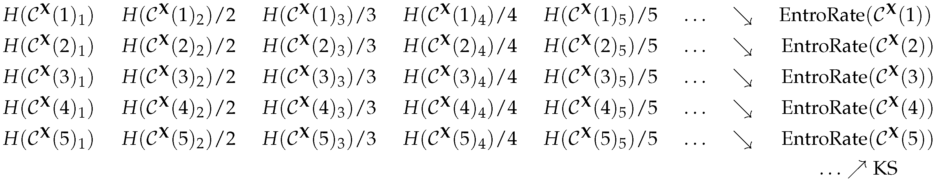
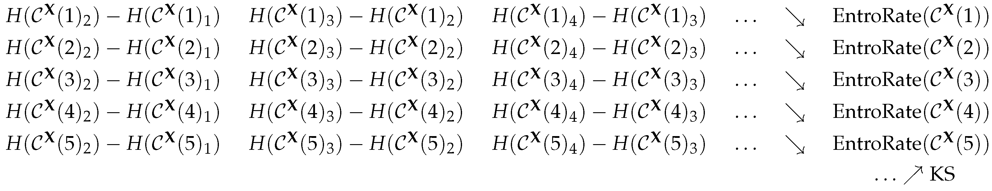
This statement shown in Antoniouk et al. [25] and generalized in [26] can be interpreted as follows: If there is no loss of information caused by the measuring process, the whole information of the process can be obtained by only considering ordinal relations between the measurements for each observable. Formula (4), to be read together with formula (3), is illustrated by Figure 1 and Figure 2, where directions of arrows indicate the direction of convergence.

2.4. Conditional Entropy of Ordinal Patterns

In order to motivate a complexity measure based on considering successive ordinal patterns, we deduce some useful inequalities from the above statement. First, fix some $d\in \mathbb{N}$ and note that, since ${(H({\mathcal{C}}^{\mathbf{X}}{(d)}_k)-H({\mathcal{C}}^{\mathbf{X}}{(d)}_{k-1}))}_{k=1}^{\infty }$ is monotonically non-increasing, it holds for all $k\in \mathbb{N}$

$$\begin{array}{ccc}\hfill H({\mathcal{C}}^{\mathbf{X}}{(d)}_k)-H({\mathcal{C}}^{\mathbf{X}}{(d)}_{k-1})& \le & \frac{1}{k}\sum _{i=1}^k(H({\mathcal{C}}^{\mathbf{X}}{(d)}_i)-H({\mathcal{C}}^{\mathbf{X}}{(d)}_{i-1}))\hfill \\ & =& \frac{1}{k}H({\mathcal{C}}^{\mathbf{X}}{(d)}_k).\hfill \end{array}$$

Because $\mathrm{EntroRate}({\mathcal{C}}^{\mathbf{X}}(d))$ is converging to the KS entropy for $d\to \infty$ in a monotonically non-decreasing way, the following is valid:

$$\begin{array}{c}\hfill \mathrm{KS}\le \underset{d\to \infty }{lim\; inf}(H({\mathcal{C}}^{\mathbf{X}}{(d)}_{k_d})-H({\mathcal{C}}^{\mathbf{X}}{(d)}_{k_d-1}))\le \underset{d\to \infty }{lim\; inf}\frac{1}{k_d}H({\mathcal{C}}^{\mathbf{X}}{(d)}_{k_d})\\ \hfill \mathrm{for}\mathrm{each}\mathrm{each}\mathrm{sequence}{(k_d)}_{d=1}^{\infty }\mathrm{of}\mathrm{natural}\mathrm{numbers}.\end{array}$$

Note that the faster the sequence ${(k_d)}_{d=1}^{\infty }$ increases, the nearer are the terms in the inequality, and good choices of the sequence provide equality of all terms in the last inequality. In particular, it holds

$$\begin{array}{c}\hfill \mathrm{KS}\le \underset{d\to \infty }{lim\; inf}(H({\mathcal{C}}^{\mathbf{X}}{(d)}_2)-H({\mathcal{C}}^{\mathbf{X}}(d))),\end{array}$$

being the background for the following definition (compare Unakafov and Keller [19]):

Definition 2.

$H({\mathcal{C}}^{\mathbf{X}}{(d)}_2)-H({\mathcal{C}}^{\mathbf{X}}(d))$ is called the Conditional entropy of ordinal patterns of order d.

Indeed, the concept given is a conditional entropy, however, since ${\mathcal{C}}^{\mathbf{X}}{(d)}_2$ is a finer partition than ${\mathcal{C}}^{\mathbf{X}}(d)$, it reduces to a difference of entropies.

2.5. Permutation Entropy

The description of KS entropy given by formula (4) includes a double-limit, where the inner one is non-increasing and the outer is non-decreasing. Bandt et al. [7] (see also [1]) have proposed the concept of Permutation entropy, which only needs one limit and was the starting point of using ordinal pattern methods. Here, the concept is given in our general context.

Definition 3.

For $d\in \mathbb{N}$, the quantity ${\mathrm{PE}}^{\mathbf{X}}(d)=\frac{1}{d}H({\mathcal{C}}^{\mathbf{X}}(d))$ is called the Permutation entropy of order d with respect to $\mathbf{X}$. Moreover, by the Permutation entropy with respect to $\mathbf{X}$, we understand ${\mathrm{PE}}^{\mathbf{X}}={lim\; sup}_{d\to \infty }{\mathrm{PE}}^{\mathbf{X}}(d)$.

The definition of Permutation entropy given is justified by the result of Bandt et al. [7] that if T is a piecewise monotone interval map, then it holds ${\mathrm{PE}}^{\mathrm{id}}=\mathrm{KS}$. Here, Ω is an interval and $\mathbf{X}=id$, where $id$ denotes the identity on Ω. We do not want to say more about this result, but mention that general equality of KS entropy and Permutation entropy is an open problem, however as shown in [25] (under the assumptions above) it holds

$$\mathrm{KS}\le {\mathrm{PE}}^{\mathbf{X}}.$$

Assuming that the increments of entropy of successive ordinal partitions are well-behaved in the sense that

$$\underset{d\to \infty }{lim}(H({\mathcal{C}}^{\mathbf{X}}(d+1))-H({\mathcal{C}}^{\mathbf{X}}(d)))$$

exists, by the Stolz–Cesàro theorem, one obtains the inequality

$$\begin{array}{ccc}\hfill \mathrm{KS}& \le & \underset{d\to \infty }{lim\; inf}(H({\mathcal{C}}^{\mathbf{X}}{(d)}_2)-H({\mathcal{C}}^{\mathbf{X}}(d)))\hfill \\ & \le & \underset{d\to \infty }{lim}(H({\mathcal{C}}^{\mathbf{X}}(d+1))-H({\mathcal{C}}^{\mathbf{X}}(d)))\hfill \\ & =& \underset{d\to \infty }{lim}(H({\mathcal{C}}^{\mathbf{X}}(d))-H({\mathcal{C}}^{\mathbf{X}}(d-1)))\hfill \\ & =& \underset{d\to \infty }{lim}\frac{1}{d}\sum _{i=1}^d(H({\mathcal{C}}^{\mathbf{X}}(i))-H({\mathcal{C}}^{\mathbf{X}}(i-1)))\hfill \\ & =& \underset{d\to \infty }{lim}\frac{1}{d}H({\mathcal{C}}^{\mathbf{X}}(d))={\mathrm{PE}}^{\mathbf{X}}\hfill \end{array}$$

(compare [19]). This inequality is shedding some light on the relationship of KS entropy, Permutation entropy and the various conditional entropy differences (see Figure 2) considered.

Summarizing, all quantities considered are related to the entropies $H({\mathcal{C}}^{\mathbf{X}}{(d)}_k)$. For simplicity, we now switch to only one observable X. The generalization is simple but not necessary for the following. In the restricted case, for $d,k\in \mathbb{N}$, it holds

$$\begin{array}{c}\hfill H({\mathcal{C}}^X{(d)}_k)=-\sum _{{({\pi }_l)}_{l=1}^k\in {\mathrm{\Pi }}_d^k}{P}_{{({\pi }_l)}_{l=1}^k}ln{P}_{{({\pi }_l)}_{l=1}^k},\end{array}$$

where

$$\begin{array}{c}\hfill P_{{}_{{({\pi }_l)}_{l=1}^k}}=P(\{\omega \in \mathrm{\Omega }\mid (X(T^{\circ l+d-1}(\omega )),\dots ,X(T^{\circ l}(\omega )),X(T^{\circ l-1}(\omega )))\\ \hfill \mathrm{has}\mathrm{ordinal}\mathrm{pattern}{\pi }_l\mathrm{for}l=1,2,\dots ,k\}).\end{array}$$

2.6. The Practical Viewpoint

Despite the general relation of KS entropy and Permutation entropy, the asymptotics of entropies taken from ordinal pattern distributions are relatively well understood by the above considerations. This allows a good interpretation of what they measure. The practical problem, however, is that asymptotics can be very slow and thus cause problems in the estimation of $P({\mathcal{C}}^{\mathbf{X}}{(d)}_k)$ from orbits of a system when d or k is high. Here, for $n,k\in \mathbb{N}$, a naive estimator of $P_{{({\pi }_l)}_{l=1}^k}$ is

$$\begin{array}{c}\hfill p_{{({\pi }_l)}_{l=1}^k}=\frac{\#\{t\in \{d+k-1,\dots ,N-1\}\mid (x_{t-i},\dots ,x_{t-i-d})\mathrm{has}\mathrm{ord}.\mathrm{patt}.{\pi }_i\mathrm{for}i=0,\dots ,k-1\}}{N-d-k+1}\end{array}$$

and a naive estimator of $H({\mathcal{C}}^X{(d)}_k)$ is

$$\begin{array}{c}\hfill h(d,k)=-\sum _{{({\pi }_l)}_{l=1}^k\in {\mathrm{\Pi }}_d^k}{p}_{{({\pi }_l)}_{l=1}^k}ln{p}_{{({\pi }_l)}_{l=1}^k}.\end{array}$$

The problem is that one needs too many measurements for a reliable estimation if d and k are large. This is demonstrated for the logistic map with “maximal chaos” in the one-dimensional case. Here, $\mathrm{\Omega }=[0,1]$, T is defined by $T(\omega )=4\omega (1-\omega )$ for $x\in [0,1]$, P is the Lebesgue measure, and X is the identity map. Note that this map and maps of the whole logistic family are often used for testing complexity measures. (For more information, see [27,28].)

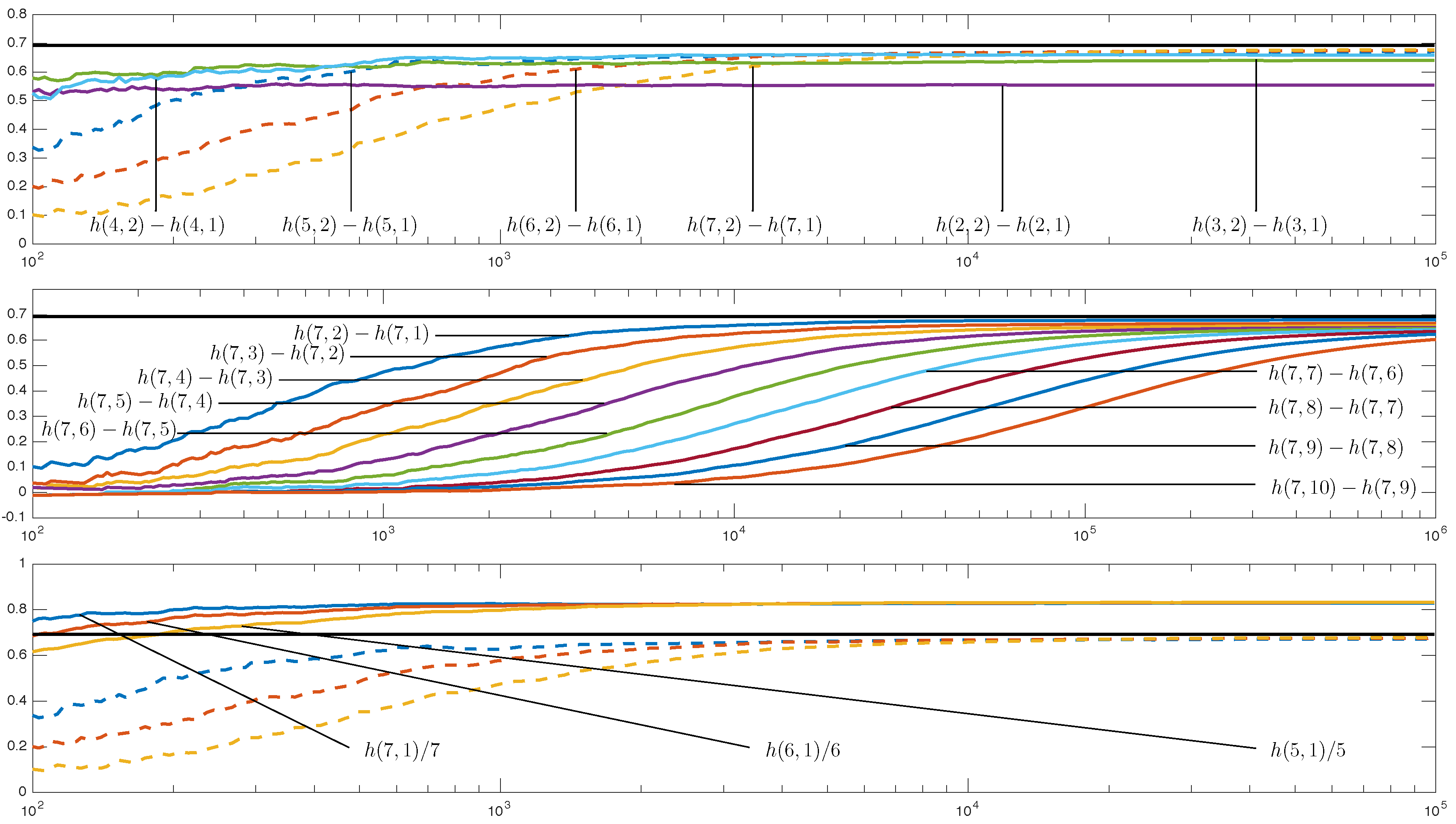
Figure 3 shows $h(d,k)-h(d,k-1)$ and $\frac{h(d,1)}{d}$ for different $d,k\in \mathbb{N}$ in dependence on orbit lengths of T between ${10}^2$, and ${10}^5$ and ${10}^6$, respectively. The horizontal black line indicates the KS entropy of T, which is $ln2$. The graphic on the top provides curves for $h(d,k)-h(d,k-1)$ for $k=2$ and $d=2,3,\dots ,7$ being estimates of the Conditional entropy of ordinal patterns of corresponding orders d. The approximation of the KS entropy is rather good for $d=7$, but a long orbit is needed. In general, the higher d is, the longer a stabilization of the estimate takes. A similar situation is demonstrated in the graphic in the middle, now with fixed $d=7$ but increasing k. In the graphic on the bottom, three of the curves from the upper graphic are drawn again as a contrast to curves showing $\frac{h(d,1)}{d}$ for $d=5,6,7$. The latter can be considered as estimates of the corresponding Permutation entropies; the estimates, however, are bad since d is not large enough. Note that according to the result of Bandt et al., estimates for very high d must be near to the KS entropy. The results illustrate that using Conditional entropy of ordinal patterns is a good compromise. Good performance of Conditional entropy of ordinal patterns for the logistic family is reported in Unakafov and Keller [19].

3. Generalizations Based on the Families of Renyi and Tsallis Entropies

3.1. The Concept

It is natural to generalize Permutation entropy to Tsallis and Renyi entropy variants, which has first been done by Zunino et al. [12]. Liang et al. [13] discuss the performances of a large list of complexity measures, among them are the classical as well as Tsallis and Renyi Permutation entropies in tracking changes of EEG during different anesthesia states. They report that the class of Permutation entropies in some features shows good performance relative to the other measures, with best results of the Renyi variant. Let us have a closer look at the new concepts.

Definition 4.

For some given positive $\alpha \ne 1$, the empirical Renyi Permutation entropy (eRPE) and empirical Tsallis Permutation entropy (eTPE) of order $d\in \mathbb{N}$ and of delay $\tau \in \mathbb{N}$ of a time series ${(x_t)}_{t=0}^{N-1}$ with $N\in \mathbb{N}$ is defined by

$$\begin{array}{cc}\hfill \mathrm{eRPE}\left(\alpha ,d,\tau ,{(x_t)}_{t=0}^{N-1}\right)& =-\frac{1}{d(1-\alpha )}ln\sum _{\pi \in {\mathrm{\Pi }}_d}{(p_{\pi }^{\tau })}^{\alpha }\hfill \end{array}$$

and

$$\begin{array}{cc}\hfill \mathrm{eTPE}\left(\alpha ,d,\tau ,{(x_t)}_{t=0}^{N-1}\right)& =-\frac{1}{d(\alpha -1)}\left(1-\sum _{\pi \in {\mathrm{\Pi }}_d}{(p_{\pi }^{\tau })}^{\alpha }\right),\hfill \end{array}$$

respectively, with $p_{\pi }$ as given in (2). (We include the factor $\frac{1}{d}$ in the entropy formulas only for reasons of comparability with the classical Permutation entropy.)

3.2. Some Properties

As, in general, the Renyi and the Tsallis entropy of a distribution for $\alpha \to 1$ converge to the Shannon entropy, convergence of eRPE and eTPE to the ePE holds as well. The two concepts principally can be used in data analysis to further emphasize the role of small ordinal pattern probabilities if $\alpha <1$ or of large ones if $\alpha >1$ (compare the graphs of the functions $x\mapsto xlnx,x\mapsto x^{\alpha }$ for different α and $x\in [0,1]$). The consequences of this weighting become obvious for the eRPE when considering limits for $\alpha \to 0$ and $\alpha \to \infty$. One easily sees that

$$\begin{array}{ccc}\hfill \underset{\alpha \to \infty }{lim}\mathrm{eRPE}\left(\alpha ,d,\tau ,{(x_t)}_{t=0}^{N-1}\right)& =& -\frac{ln({max}_{\pi \in {\mathrm{\Pi }}_d}{p}_{\pi }^{\tau })}{d}\hfill \\ \hfill \underset{\alpha \to 0}{lim}\mathrm{eRPE}\left(\alpha ,d,\tau ,{(x_t)}_{t=0}^{N-1}\right)& =& \frac{ln(\#\{\pi \in {\mathrm{\Pi }}_d\mid p_{\pi }^{\tau }\ne 0\})}{d},\hfill \end{array}$$

meaning that for large α, the eRPE mainly measures the largest relative ordinal pattern frequency (on a logarithmic scale), with low entropy for high relative frequency; for small α, the eRPE mainly measures the number of occurring ordinal patterns (on a logarithmic scale). Since

$$\mathrm{eTPE}\left(\alpha ,d,\tau ,{(x_t)}_{t=0}^{N-1}\right)=\frac{{\mathrm{e}}^{d(1-\alpha )\mathrm{eRPE}\left(\alpha ,d,\tau ,{(x_t)}_{t=0}^{N-1}\right)}-1}{d(1-\alpha )},$$

the eTPE is only a monotone functional of the eRPE for fixed α; despite a different scale, it has similar properties as the eRPE.

For $\alpha =2$, the eRPE has a nice interpretation. Having $N_{\pi }=(N-d\tau )p_{\pi }^{\tau }$ in the time series, there are $\frac{N_{\pi }(N_{\pi }-1)}{2}$ pairs of different times providing ordinal pattern π. Since, all in all, we have $\frac{(N-d\tau )(N-d\tau -1)}{2}$ different time pairs, the quantity

$$\begin{array}{c}\hfill \frac{{\sum }_{\pi \in {\mathrm{\Pi }}_d}{N}_{\pi }(N_{\pi }-1)}{(N-d\tau )(N-d\tau -1)}=\frac{{\sum }_{\pi \in {\mathrm{\Pi }}_d}{N}_{\pi }^2-(N-d\tau )}{{(N-d\tau )}^2-(N-d\tau )}\approx \sum _{\pi \in {\mathrm{\Pi }}_d}{(p_{\pi }^{\tau })}^2\end{array}$$

can be interpreted as the degree of recurrence in the time series. This quantity is, in fact, the symbolic correlation integral recently introduced by Caballero et al. [29].

3.3. Demonstration

We demonstrate the performance of eRPE and eTPE for different α on the base of EEG data discussed in [6]. For this, we consider two parts each of a 19-channel scalp EEG of a boy with lesions predominantly in the left temporal lobe caused by a connatal toxoplasmosis. The data were sampled at a rate of 256 Hz, meaning that 256 measurements were obtained each second. The first data part (data set 1) was taken from an EEG derived at an age of eight years and the second one (data set 2) was derived at an age of 11 years, four months after the implantation of a vagus stimulator. Note that epileptic activity was significant before vagus stimulation and was the reason for the implantation. (For some more details on the data, see [6]).

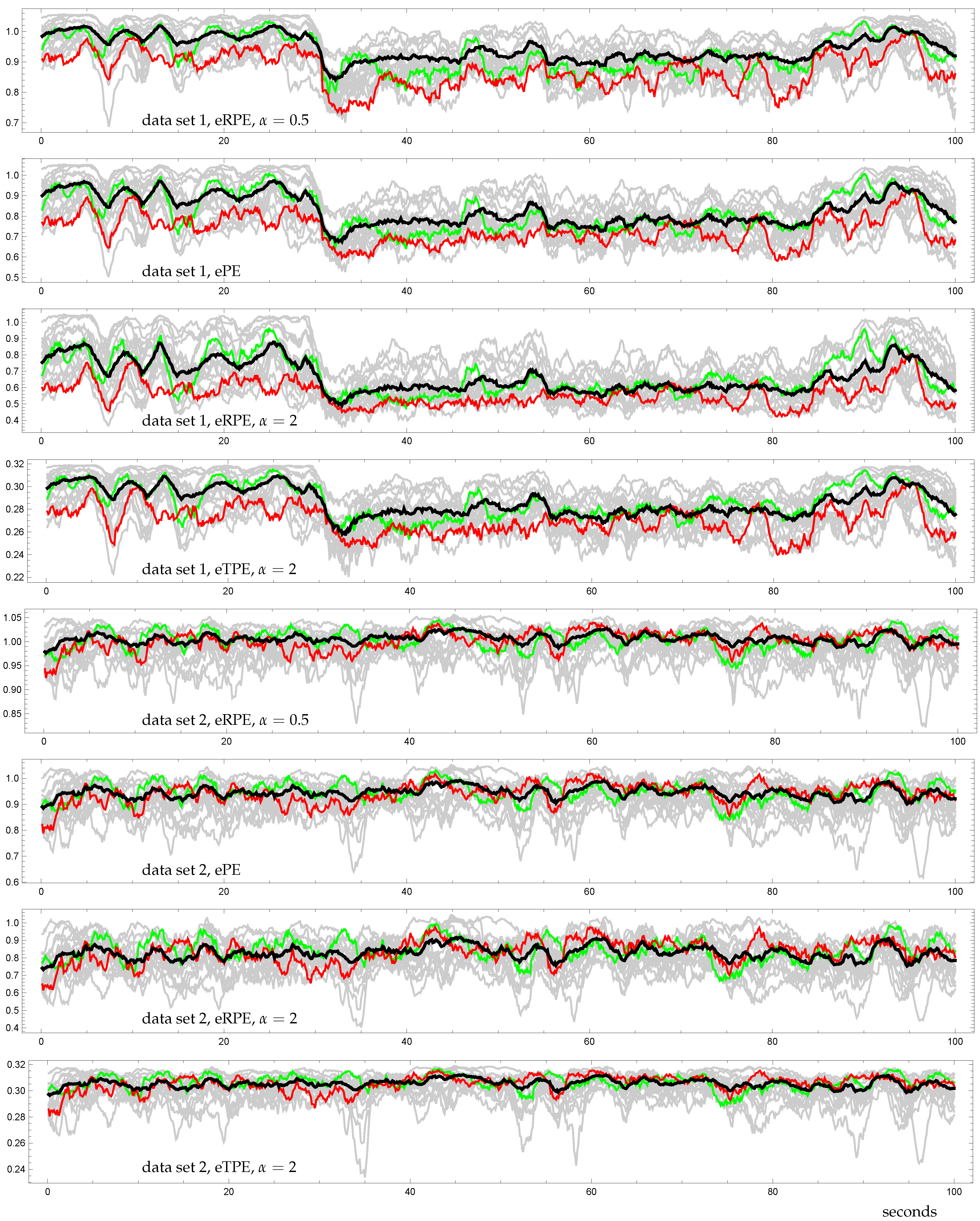
Figure 4 shows ePE and eRPE for $\alpha =0.5,2$ and eTPE for $\alpha =2$ for the two data sets in dependence on a shifted time window, where $d=3$ and $\tau =4$. Each graphic represents the 19 channels for a fixed entropy by 19 entropy curves. Among the channels are T3 and P3, which are interesting in the following. The curve related to a fixed channel contains pairs $(t,h_t)$, where $h_t$ is the entropy of the segment of the related time series ending at time t and containing $2\times 256+3\times 4$ successive measurements. (Each segment provides $512=2\times 256$ ordinal patterns representing a time segment of two seconds.) The t are chosen from a time segment of 100 seconds, where the beginning time is set to 0 for simplicity. We have added a fat black curve representing the entropy of the whole brain instead of the single channels. Here, the relative frequencies used for entropy determination were obtained by counting ordinal patterns in the considered time segment pooled over all channels.

The two EEG parts reflect changes of brain dynamics. Whereas the first EEG part shows low entropies relative to the other channels of P3 and, partially, of T3, entropies of both channels are relatively higher in the second EEG part. More information with additional data sets derived directly before and after the vagus stimulator implantation is available from [6], where only the ePE was considered. Here, we want to note that P3 and T3 are from the left part of the brain with the lesions, and P3 seems to mainly reflect some kind of irregular behavior related to them. The most interesting point is that before vagus stimulator implantation, P3 and partially T3 are conspicuous both in phases with and without epileptic activity. For orientation, the graphics given in Figure 4 for data set 1 and in Figure 5 show a part from around 30 to 90 seconds with low entropies for pooled ordinal patterns (fat black curve) related to a generalized epileptic seizure, meaning epileptic activity in the whole brain.

Figure 4 suggests that a visual inspection of the data using eRPE and eTPE instead of ePE does not seem to gain further insights when α is chosen close to 1. Here, it is important to note that, for the parameters considered, all ordinal patterns are accessed at many times (with some significant frequency). Our guess is supported by

Table 1. Concordance of the sign of entropy differences of ePE and eRPE for given α.

α	$0.5$	$0.8$	$0.9$	$1.1$	$1.2$	$1.5$	2	250
Fp2	$98.69\%$	$99.52\%$	$99.77\%$	$99.78\%$	$99.58\%$	$99.05\%$	$98.38\%$	$94.85\%$
T3	$95.41\%$	$98.39\%$	$99.22\%$	$99.26\%$	$98.59\%$	$96.92\%$	$95.20\%$	$89.31\%$
P3	$93.18\%$	$97.71\%$	$98.93\%$	$99.05\%$	$98.21\%$	$96.30\%$	$94.33\%$	$83.66\%$

. For each of the channels FP2, T3, and P3 and given α, the relative frequency of concordant pairs of the observations ePE, eRPE at time s and ePE, eRPE at time t among all pairs $(s,t);s<t$ is shown. $(s,t)$ is said to be concordant if the difference between ePE at times s and t and the difference between eRPE at times s and t have the same sign.

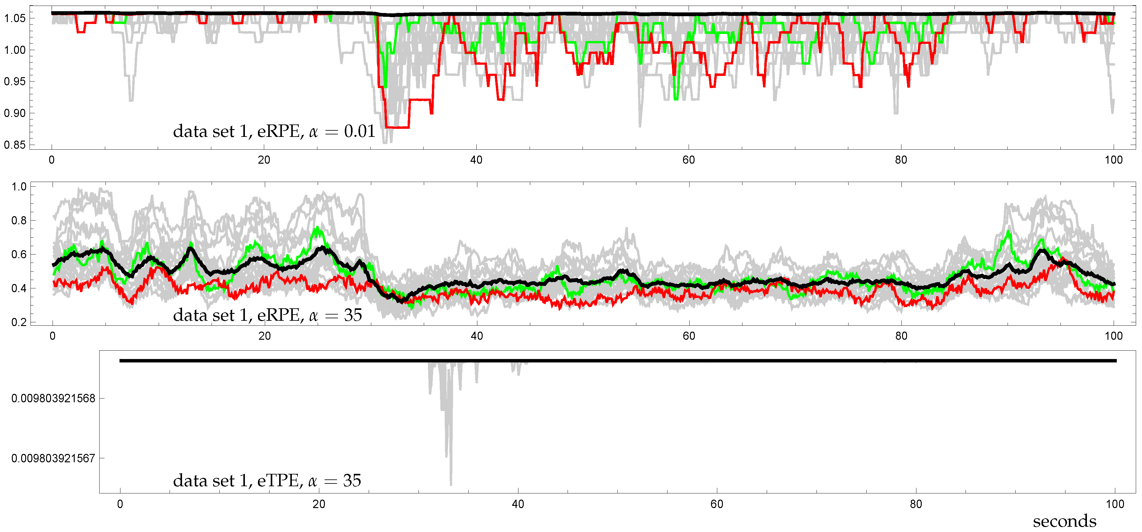
The results particularly reflect the fact that for channel Fp2, providing measurements from the front of the brain, the ordinal patterns are more equally distributed than for T3; and for P3, the distribution of ordinal patterns is the farthest from equidistribution. For contrast, we also consider $\alpha =250$. Figure 5 related to data set 1 indicates that extreme choices of α could be useful in order to analyze and visualize changes in the brain dynamics more forcefully. The upper graphic of eRPE for $\alpha =0.01$ shows that at the beginning of an epileptic seizure, the number of ordinal patterns abruptly decreases for nearly all channels and after some increasing stays on a relatively low level until the end of the seizure. For $\alpha =35$, it is interesting to look at the whole ensemble of the entropies.

Here, eRPE indicates much more variability of the largest ordinal pattern frequencies of the channels in the seizure-free parts than in the seizure epochs. The very low entropy at the beginning of the seizure reverts back to mainly increasing or decreasing only ordinal patterns. Here, the special kind of scaling given by the eTPE allows to emphasize the special situation at the beginning of a seizure and can therefore be interesting for an automatic detection of epileptic seizures, whereby the correct tuning of α is important.

4. Classification on the Base of Different Entropies

Classification is an important issue in the analysis of EEG data, for which in many cases entropy measures can be exploited. Here, it is often unclear which of these measures are the best and how much they are ‘overlapping’. In view of the discussion in Section 2, note that by the asymptotic statements considered, ordinal pattern based measures can behave very similarly for high orders, but for low orders their performance can be rather different. Also including different delays in the analysis, one obtains much flexibility on one hand, but the problem of a high number of parameter combinations arises on the other hand.

Here, we want to discuss the classification of EEG data using ePE, empirical Conditional entropies of ordinal patterns (eCE, see below) and, additionally, Approximate entropy (ApEn) (see Pincus [30]) and Sample entropy (SampEn) (see Richmann and Moormann [31], and extending work in Keller et al. [10]). For the definition and usage of ApEn and SampEn, in particular for the parameter choice (“$\mathrm{ApEn}(2,0.2\sigma ,\mathbf{x})$”, “$\mathrm{SampEn}(2,0.2\sigma ,\mathbf{x})$”), we directly refer to [10]. The eCE, motivated and defined for dynamical systems in Section 2, is given by the following definition (compare also [10]):

Definition 5.

Given a time series ${(x_t)}_{t=0}^{N-1}$ with $N\in \mathbb{N}$, the quantity

$$\begin{array}{cc}\hfill \mathrm{eCE}\left(d,\tau ,{(x_t)}_{t=0}^{N-1}\right)& =\sum _{\pi \in {\mathrm{\Pi }}_d}{p}_{\pi }^{\tau }ln{p}_{\pi }^{\tau }-\sum _{{\pi }_1,{\pi }_2\in {\mathrm{\Pi }}_d}{p}_{{\pi }_1,{\pi }_2}^{\tau }ln{p}_{{\pi }_1,{\pi }_2}^{\tau }\hfill \end{array}$$

is called empirical Conditional entropy of ordinal patterns (eCE) of order $d\in \mathbb{N}$ and of delay $\tau \in \mathbb{N}$, where $p_{\pi }^{\tau }$ is defined by (2) and $p_{{\pi }_1,{\pi }_2}^{\tau }$ by

$$\begin{array}{cc}\hfill p_{{\pi }_1,{\pi }_2}^{\tau }& =\frac{1}{N-d\tau -1}\#\{t\in \{d\tau ,d\tau +1,\dots ,N-2\}\mid \hfill \\ & (x_t,x_{t-\tau },\dots ,x_{t-d\tau }),(x_{t+1},x_{t+1-\tau },\dots ,x_{t+1-d\tau })haveordinalpatterns{\pi }_1,{\pi }_2\}\hfill \end{array}$$

Note that for each time series ${(x_t)}_{t=0}^{N-1}$ and each $d\in \mathbb{N}$, it holds $\mathrm{eCE}\left(d,1,{(x_t)}_{t=0}^{N-1}\right)=h(d,2)-h(d,1)$. So $\mathrm{eCE}\left(d,1,{(x_t)}_{t=0}^{N-1}\right)$ is an estimate of the Conditional entropy of ordinal patterns defined in Section 2.

4.1. The Data

The considered EEG data are recordings from the Bonn EEG Database [20], each of a length of $23.6$ s recorded at a sampling rate of $173.61$ Hz. The data consists of five groups, each of 100 recordings:

• group A: surface EEG’s recorded from healthy subjects with open eyes,
• group B: surface EEG’s recorded from healthy subjects with closed eyes,
• group C: intracranial EEG’s recorded from subjects with epilepsy during a seizure-free period from within the epileptogenic zone,
• group D: intracranial EEG’s recorded from subjects with epilepsy during a seizure-free period from hippocampal formation of the opposite hemisphere of the brain,
• group E: intracranial EEG’s recorded from subjects with epilepsy during a seizure period.

In contrast to [10], where the groups A and B and the groups C and D were pooled, each of the groups is considered separately in the following.

4.2. Visualization and Classification for Delay One

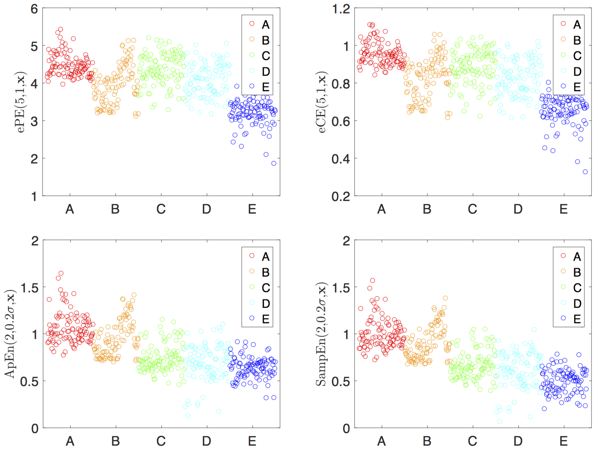
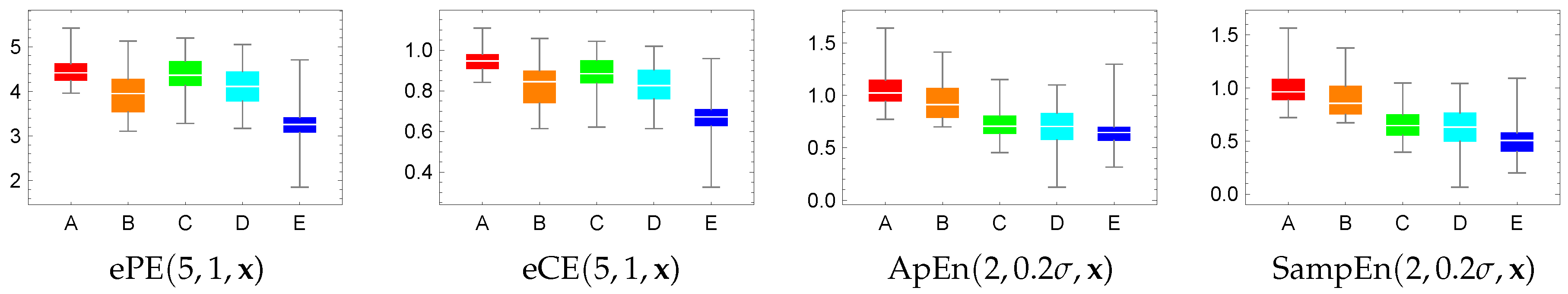
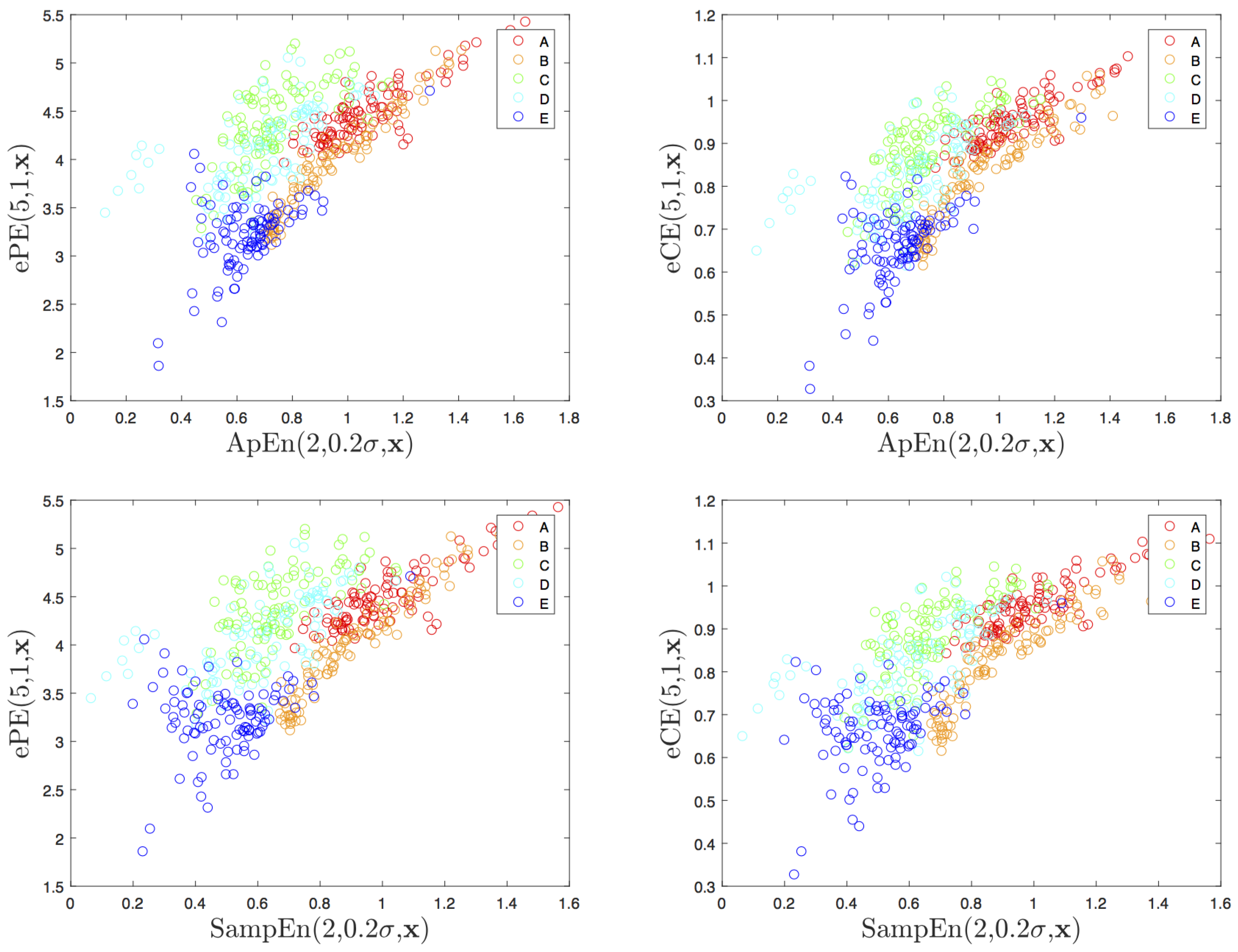
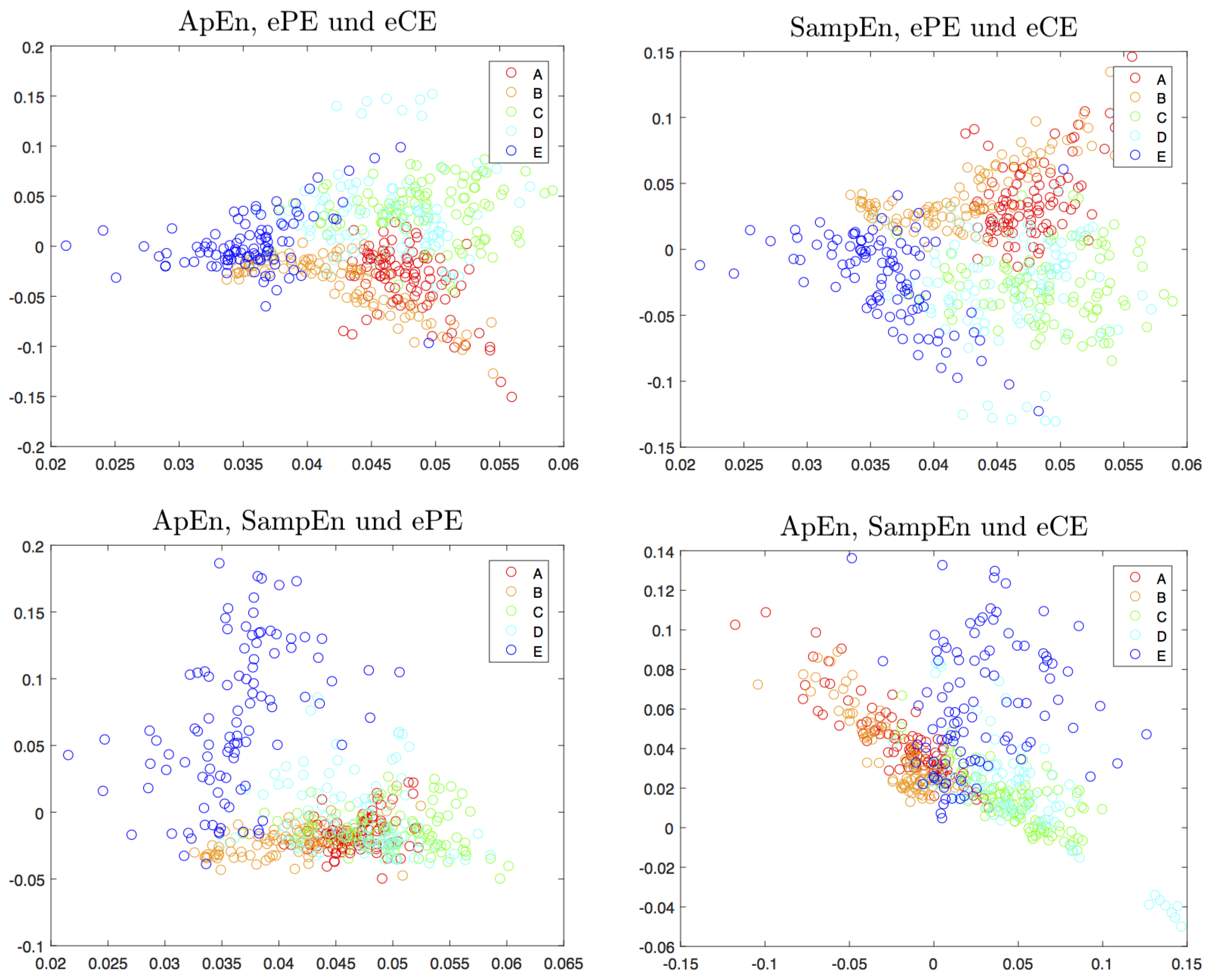
In order to give a visual impression of how the considered entropies separate the data, we provide three figures. For the ordinal pattern based measures, we have chosen order $d=5$ and delay $\tau =1$. Figure 6 shows the values of the four considered entropies for all data sets. The values obtained are drawn from the left to the right starting from those from group A and ending with those from group E. For better presentation of the distribution of all entropies, we have added boxplots (see Figure 7). Figure 6 shows that each of the considered entropies does not separate much, however, one can see different kinds of separation properties for the ordinal pattern based entropies and the two other entropies. A better separation is seen in Figure 8 where one entropy measure is plotted versus another one, in four different combinations. Here, the discrimination between E, the union of A and B, and the union of C and D is rather good, confirming the results in [10], but both $A,B$ and $C,D$ are strongly overlapping. The general separation seems to be slightly better using three entropies, which is illustrated by Figure 9. Here, however, a two-dimensional representation is chosen by plotting the second principal component versus the first one, both obtained by principal component analysis from the three entropy components’ variables.

In order to obtain more objective and reliable results, we have tested a classification of the data on the base of the chosen entropies and of Random Forests (see Breiman [32]), a popular and efficient machine learning method. For this purpose, the data were randomly divided into a learning group consisting of $80\%$ of the data sets and a testing group consisting of the remaining $20\%$. The obtained accuracy of the classification, i.e., the relative frequency of the correctly classified data sets, was averaged over 1000 testing trials for each entropy combination considered. The results of this procedure, summarized in

Table 2. Results of the classification on the base of one entropy.

Entropy	Classification Accuracy (In %)
ApEn	31.0
SampEn	37.8
ePE	32.0
eCE	30.0

,

Table 3. Results of the classification on the base of two entropies.

Entropy	Classification Accuracy (In %)
ApEn & SampEn	51.0
ApEn & ePE	58.0
ApEn & eCE	61.8
SampEn & ePE	64.0
SampEn & eCE	64.6
ePE & eCE	48.2

and

Table 4. Results of the classification on the base of three entropies.

Entropy	Classification Accuracy (In %)
ApEn & SampEn & ePE	67.4
ApEn & SampEn & eCE	66.8
ApEn & ePE & eCE	65.4
SampEn & ePE & eCE	71.8

, show that including an additional entropy results in a higher accuracy, but that the way in which entropies are combined is crucial for the results. Note that combining all four entropies provides an accuracy of only $70.6\%$.

4.3. Other Delays

Clearly, the accuracy of the classification using ePE and eCE depends on the choice of the parameters of the entropies. Whereas the choice of higher orders does not make sense for statistical reasons, as already mentioned in Section 2, testing different delays τ is useful since the delay contains important scale information. Note that already for both, ePE and eCE, the classification accuracy varies by more then $14\%$. Considering only delays $\tau =1,2,\dots ,9$ for $d=5$, the maximal accuracies for ePE and eCE are $45.01\%$ and $48.0\%$ for $\tau =6$ and $\tau =5$, respectively. Note that both results are better than those for the SampEn (see Table 2) and that $\tau =1$ provides the worst results. Combining two ePEs and eCEs for delays in $\{1,2,\dots ,9\}$, one reaches an accuracy of $61.79\%$ (for delays 1 and 2) and $62.28\%$ (for delays 1 and 9), respectively.

5. Resume

Throughout this paper, we have discussed ordinal pattern based complexity measures both from the viewpoint of their theoretical foundation and their application in EEG analysis, centered upon Permutation entropy and its conditional variants. We have pointed out that, as in many situations in (model-based) data analysis, one must give attention to the discrepancy of theoretical asymptotics and statistical requirements, here in view of estimating KS entropy. In the case of moderately but not extremely long data sets, the concept of Conditional entropy of ordinal patterns, as discussed, could be a compromise. It has been shown to have better performance than the classical Permutation entropy in many situations.

A good way of further investigating the performances of ordinal pattern based measures is an extensive testing of these measures for data classification. In this direction, the results of this paper for a restricted parameter choice are already promising, however systematic studies are required and planned. For this purpose, based on the considerations in Section 3 and Section 4, the authors also propose including Renyi and Tsallis variants of Permutation entropy (with an extreme parameter choice), ordinal pattern based disequilibrium measures as considered by Zunino et al. [17] and Zunino and Ribeiro [18]), and classical concepts such as Approximate entropy and Sample entropy. The latter are interesting in combination with ordinal complexity measures since they possibly address other features. The most important challenge, however, is to deal with the great number of entropy measures and parameters which, in the opinion of the authors, can be faced by using machine learning ideas in a sophisticated way.

References

- Bandt, C.; Pompe, B. Permutation entropy—A natural complexity measure for time series. Phys. Rev. E 2002, 88, 174102. [Google Scholar] [CrossRef] [PubMed]
- Amigó, J.M.; Keller, K.; Kurths, J. (Eds.) Recent progress in symbolic dynamics and permutation complexity. Ten years of permutation entropy. Eur. Phys. J. Spec. Top. 2013, 222, 247–257.
- Zanin, M.; Zunino, L.; Rosso, O.A.; Papo, D. Permutation entropy and its main biomedical and econophysics applications: A review. Entropy 2012, 14, 1553–1577. [Google Scholar] [CrossRef]
- Amigó, J.M.; Keller, K.; Unakafova, V.A. Ordinal symbolic analysis and its application to biomedical recordings. Philos. Trans. R. Soc. A 2015, 373, 20140091. [Google Scholar] [CrossRef] [PubMed]
- Amigó, J.M. Permutation Complexity in Dynamical Systems; Springer: Berlin-Heidelberg, Germany, 2010. [Google Scholar]
- Keller, K.; Lauffer, H. Symbolic analysis of high-dimensional time series. Int. J. Bifurc. Chaos 2003, 13, 2657–2668. [Google Scholar] [CrossRef]
- Bandt, C.; Keller, G.; Pompe, B. Entropy of interval maps via permutations. Nonlinearity 2002, 15, 1595–1602. [Google Scholar] [CrossRef]
- Liu, X.-F.; Wang, Y. Fine-grained permutation entropy as a measure of natural complexity for time series. Chin. Phys. B 2009, 18, 2690–2695. [Google Scholar]
- Fadlallah, B.; Chen, B.; Keil, A.; Príncipe, J. Weighted-permutation entropy: A complexity measure for time series incorporating amplitude information. Phys. Rev. E 2013, 87, 022911. [Google Scholar] [CrossRef] [PubMed]
- Keller, K.; Unakafov, A.M.; Unakafova, V.A. Ordinal Patterns, Entropy, and EEG. Entropy 2014, 16, 6212–6239. [Google Scholar] [CrossRef]
- Bian, C.; Qin, C.; Ma, Q.D.Y.; Shen, Q. Modified permutation-entropy analysis of heartbeat dynamics. Phys. Rev. E 2012, 85, 021906. [Google Scholar] [CrossRef] [PubMed]
- Zunino, L.; Perez, D.G.; Kowalski, A.; Martín, M.T.; Garavaglia, M.; Plastino, A.; Rosso, O.A. Brownian motion, fractional Gaussian noise, and Tsallis permutation entropy. Physica A 2008, 387, 6057–6068. [Google Scholar] [CrossRef]
- Liang, Z.; Wang, Y.; Sun, X.; Li, D.; Voss, L.J.; Sleigh, J.W.; Hagihira, S.; Li, X. EEG entropy measures in anesthesia. Front. Comput. Neurosci. 2015, 9, 00016. [Google Scholar] [CrossRef] [PubMed]
- Li, D.; Li, X.; Liang, Z.; Voss, L.J.; Sleigh, J.W. Multiscale permutation entropy analysis of EEG recordings during sevoflurane anesthesia. J. Neural Eng. 2010, 7, 046010. [Google Scholar] [CrossRef] [PubMed]
- Ouyang, G.; Li, J.; Liu, X.; Li, X. Dynamic characteristics of absence EEG recordings with multiscale permutation entropy analysis. Epilepsy Res. 2013, 104, 246–252. [Google Scholar] [CrossRef] [PubMed]
- Azami, H.; Escudero, J. Improved multiscale permutation entropy for biomedical signal analysis: Interpretation and application to electroencephalogram recordings. Biomed. Signal Process. 2016, 23, 28–41. [Google Scholar] [CrossRef]
- Zunino, L.; Soriano, M.C.; Rosso, O.A. Distinguishing chaotic and stochastic dynamics from time series by using a multiscale symbolic approach. Phys. Rev. E 2012, 86, 046210. [Google Scholar] [CrossRef] [PubMed]
- Zunino, L.; Ribeiro, H.V. Discriminating image textures with the multiscale two-dimensional complexity-entropy causality plane. Chaos Solitons Fract. 2016, 91, 679–688. [Google Scholar] [CrossRef]
- Unakafov, A.M.; Keller, K. Conditional entropy of ordinal patterns. Physica D 2013, 269, 94–102. [Google Scholar] [CrossRef]
- Andrzejak, R.G.; Lehnertz, K.; Rieke, C.; Mormann, F.; David, P.; Elger, C.E. Indications of nonlinear deterministic and finite dimensional structures in time series of brain electrical activity: Dependence on recording region and brain state. Phys. Rev. E 2001, 64, 061907. [Google Scholar] [CrossRef] [PubMed]
- Unakafova, V.A.; Keller, K. Efficiently Measuring Complexity on the Basis of Real-World Data. Entropy 2013, 15, 4392–4415. [Google Scholar] [CrossRef]
- Walters, P. An Introduction to Ergodic Theory; Springer: New York, NY, USA, 1982. [Google Scholar]
- Takens, F. Detecting strange attractors in turbulence. In Lecture Notes in Mathematics; Dynamical Systems and Turbulence; Rand, D.A., Young, L.S., Eds.; Springer: New York, NY, USA, 1981; Volume 898, pp. 366–381. [Google Scholar]
- Gutman, J. Takens’ embedding theorem with a continuous observable. arXiv 2016. [Google Scholar]
- Antoniouk, A.; Keller, K.; Maksymenko, S. Kolmogorov-Sinai entropy via separation properties of order-generated σ-algebras. Discrete Contin. Dyn. Syst. A 2014, 34, 1793–1809. [Google Scholar]
- Keller, K.; Maksymenko, S.; Stolz, I. Entropy determination based on the ordinal structure of a dynamical system. Discrete Contin. Dyn. Syst. B 2015, 20, 3507–3524. [Google Scholar] [CrossRef]
- Sprott, J.C. Chaos and Time-Series Analysis; Oxford University Press: Oxford, UK, 2003. [Google Scholar]
- Young, L.-S. Mathematical theory of Lyapunov exponents. J. Phys. A Math. Theor. 2013, 46, 1–17. [Google Scholar] [CrossRef]
- Caballero, M.V.; Mariano, M.; Ruiz, M. Draft: Symbolic Correlation Integral. Getting Rid of the Proximity Parameter. Available online: http://data.leo-univ-orleans.fr/media/seminars/175/WP_208.pdf (accessed on 14 February 2017).
- Pincus, S.M. Approximate entropy as a measure of system complexity. Proc. Natl. Acad. Sci. USA 1991, 88, 2297–2301. [Google Scholar] [CrossRef] [PubMed]
- Richman, J.S.; Moorman, J.R. Physiological time-series analysis using approximate entropy and sample entropy. Am. J. Physiol. Heart Circ. Physiol. 2000, 278, 2039–2049. [Google Scholar]
- Breiman, L. Random forests. Mach. Learn. 2001, 45, 5–32. [Google Scholar] [CrossRef]
Figure 1.
Approximation of Kolmogorov–Sinai (KS) entropy: the direct way.
Figure 2.
Approximation of KS entropy: the conditional way.
Figure 3.
Different estimates of the KS entropy of for different orbit lengths. On the top: for ; in the middle: for ; on the bottom: versus for .
Figure 4.
Comparison of empirical Renyi Permutation entropy (eRPE) for , 2, empirical Tsallis Permutation entropy (eTPE) for and ePE, computed from EEG recordings before stimulator implantation (data set 1) and after stimulator implantation (data set 2) for 19 channels using a shifted time window, order and delay . Highlighting, in particular, the channels T3 (green line) and P3 (red line) as well as the entropy over all channels by a fat black line. The sampling rate is 256 Hz.
Figure 5.
eRPE for , 35 and eTPE for computed from data set 1 for 19 channels using a shifted time window, and (cf. Figure 4). T3: green line, P3: red line.
Figure 6.
Entropy of the EEG data sorted by groups for four different entropy measures.
Figure 7.
Boxplots for four different entropy measures sorted by groups.
Figure 8.
One entropy versus another entropy for four entropy combinations.
Figure 9.
Second principal component versus the first one obtained from principal component analysis on three entropy variables.