Scaling Relations of Lognormal Type Growth Process with an Extremal Principle of Entropy

Abstract

The scale, inflexion point and maximum point are important scaling parameters for studying growth phenomena with a size following the lognormal function. The width of the size function and its entropy depend on the scale parameter (or the standard deviation) and measure the relative importance of production and dissipation involved in the growth process. The Shannon entropy increases monotonically with the scale parameter, but the slope has a minimum at $\sqrt{6}/6$. This value has been used previously to study spreading of spray and epidemical cases. In this paper, this approach of minimizing this entropy slope is discussed in a broader sense and applied to obtain the relationship between the inflexion point and maximum point. It is shown that this relationship is determined by the base of natural logarithm $e\simeq 2.718$ and exhibits some geometrical similarity to the minimal surface energy principle. The known data from a number of problems, including the swirling rate of the bathtub vortex, more data of droplet splashing, population growth, distribution of strokes in Chinese language characters and velocity profile of a turbulent jet, are used to assess to what extent the approach of minimizing the entropy slope can be regarded as useful.

1. Introduction

Growth phenomena or equivalent growth phenomena exist in many natural and technological processes and most often involve competitive production and dissipation mechanisms to make the size grow initially and finally decay. Examples are growth of the size of living issues such as the height of human body [1], expansion of firms and industries [2], spreading of communicable epidemics [3], production of kinetic energy during transition from laminar flow to turbulent flow [4], generation of droplets during spray process [5], population and pollution growth [6], etc.

The growth rate for such phenomena is generally proportional to the current size. According to Gibrat law, the size for such a growth process may follow a lognormal function [2]

$$f\left(t\right)=\frac{1}{\sqrt{2\pi }\sigma t}exp\left(-\frac{{(ln\frac{t}{t_D}-{\sigma }^2)}^2}{2{\sigma }^2}\right).$$

(1)

The lognormal function is very popular and important in science and technology [7,8].

There are apparently two free parameters: $t_D$ and σ. The maximum of $f\left(t\right)$ is at $t=t_D$ while σ is the scale parameter (a measure of the geometrical standard deviation) that characterizes the width of the distribution $f\left(t\right)$.

Here, t is simply called time, though sometimes it may refer to distance or other variables over which f is distributed or with which f varies. For instance, in droplet splashing, t is the diameter of droplets produced during splashing and $f\left(t\right)$ is the probability for a droplet to have size t.

For the specific problem of droplet splashing, the use of Shannon entropy determines the free parameter σ to be [9]

$$\sigma =\frac{\sqrt{6}}{6}\simeq 0.41,$$

(2)

and the way of obtaining this was attributed to the principle of maximal rate of entropy production [10,11]. Martyushev and Seleznev [12] outlined the restrictions for correct use of this principle, and commented on recent achievements as reported in [13,14,15,16,17]. Though the way of reference [9] to work with Shannon entropy production may not be linked to the principle of maximal rate of entropy production in its strict sense, the value (2) was supported by a large amount of data from droplet splashing by Wu [9] and Moreira et al. [18] using the experimental data of several publications [5,19,20]. Moreover, with this theoretical value of σ, Wang et al. [21] successfully modelled the number of hospitalized cases during the epidemics of SARS in 2003.

The lognormal function has an inflexion point (denoted $t_L$) and a maximum point (denoted $t_D$), as can be seen from Figure 1. For application to epidemic spreading [21], the value (2) is used in (1) to give

$$\frac{t_D}{t_L}\simeq 1.646,\frac{f\left(t_D\right)}{f\left(t_L\right)}\simeq 2.12,$$

(3)

and it is found that Equation (3) predicts the date and number of maximum hospitalized cases with a reasonable accuracy for SARS in the year 2003.

The spray process studied in [9,18] and the epidemics studies in [21] are two quite different problems, while the values of σ for these cases are all closely equal to that given by (2). This would mean that the method should have some broader sense. Thus, we try to explore in this paper more properties of the approach used in [9,21], and to test more cases in order to assess whether this approach can be applied in various problems.

It was claimed in [9,21] that the principle of maximum rate of entropy production is used while obtaining (2). It is necessary to verify here whether it is a maximization or minimization of some entropy property. Sensitivity analysis is also required to show whether the results are sensitive or insensitive to the choice of σ. It is also desired here that the ratios of the locations and sizes between the maximum point and inflexion point should have some form more exquisite than given by (3). Moreover, we wish that the results, such as the values of the ratios $\frac{t_D}{t_L}$ and $\frac{f\left(t_D\right)}{f\left(t_L\right)},$ should have some relationship similar to a more understandable principle such as a minimal surface energy principle. These issues will be discussed in Section 2 of this paper.

In Section 3, we provide a selective number of cases to test if the theoretical values of the ratios $\frac{t_D}{t_L}$ and $\frac{f\left(t_D\right)}{f\left(t_L\right)}$ are useful in more situations other than those considered in [9,21]. These cases include the swirling rate of the bathtub vortex, more data of droplet splashing, population growth, distribution of strokes in Chinese language characters and the velocity profile of a turbulent jet. Some discussion will also be provided to open a question about the value of the Karman constant in turbulence flow.

2. The Method of Minimal Slope of Shannon Entropy

In this section, we first study the variation of Shannon entropy with respect to the scale parameter σ and establish some relations between the locations and sizes of the inflexion point and maximum point of (1). Then, we make some sensitivity analysis. The method for application will be provided in Section 3.

2.1. Shannon Entropy Property and Some Useful Relations

For (1), it follows that

$$\frac{df\left(t\right)}{dt}=-\frac{ln\frac{t}{t_D}}{t{\sigma }^2}f(t,\sigma )$$

(4)

and

$$\frac{d^{2}f\left(t\right)}{d{t}^2}=\frac{{\sigma }^{2}ln\frac{t}{t_D}-{\sigma }^2+{ln}^2\frac{t}{t_D}}{t^2{\sigma }^4}f(t,\sigma ).$$

(5)

The inflexion point $t=t_L$ is given by $\frac{d^{2}f\left(t_L\right)}{d{t}^2}=0$. Thus,

$${\sigma }^{2}ln\frac{t_L}{t_D}-{\sigma }^2+{ln}^2\frac{t_L}{t_D}=0.$$

(6)

This equation can be solved for $\frac{t_D}{t_L}$ to give

$$\left\{\begin{array}{c}\frac{t_D}{t_L}=\varphi \left(\sigma \right)\hfill \\ \varphi \left(\sigma \right)=e^{\frac{1}{2}\sigma \left(\sigma +\sqrt{{\sigma }^2+4}\right)}\hfill \end{array}.\right.$$

(7)

Furthermore,

$$f\left(t_L\right)=\frac{1}{\sqrt{2\pi }\sigma t_L}exp\left(-\frac{{(ln\frac{t_L}{t_D}-{\sigma }^2)}^2}{2{\sigma }^2}\right),f\left(t_D\right)=\frac{1}{\sqrt{2\pi }\sigma t_D}exp\left(-\frac{{\sigma }^2}{2}\right).$$

The use of these two relations and of expression (7) for $\frac{t_L}{t_D}$ gives

$$\left\{\begin{array}{c}\frac{f\left(t_D\right)}{f\left(t_L\right)}=\psi \left(\sigma \right)\hfill \\ \psi \left(\sigma \right)=exp\left(-{\sigma }^2-\frac{\sqrt{4{\sigma }^2+{\sigma }^4}}{2}+\frac{1}{2}{\left(\frac{3\sigma }{2}+\frac{\sqrt{4+{\sigma }^2}}{2}\right)}^2\right)\hfill \end{array}.\right.$$

(8)

Recall that expressions (7) and (8) have already been obtained in [21] for epidemic spreading.

The Shannon entropy for Equation (1) is defined here as

$$S\left(\sigma \right)=-{\int }_0^{\infty }{t}^{1-3}f\left(t\right)ln\left(t^{1-3}f\left(t\right)\right)d{t}^3.$$

(9)

See Section 2.2 for more details of the choice of the power $t^3$ and Dumouchel [22] for discussions and more references. The explicit form for Equation (9) is

$$S\left(\sigma \right)=3\left(ln\left(\sqrt{2\pi }\sigma \right)+3\left({lnt}_D+{\sigma }^2\right)+\frac{1}{2}\right).$$

(10)

For convenience, we put $S\left(\sigma \right)=S_V\left(\sigma \right)+9{lnt}_D$, where $S_V\left(\sigma \right)=3\left(ln\left(\sqrt{2\pi }\sigma \right)+3{\sigma }^2+\frac{1}{2}\right)$ is solely dependent on σ. If $t_D$ is regarded as constant independent of σ, then

$$S^{\prime }\left(\sigma \right)\equiv \frac{dS\left(\sigma \right)}{d\sigma }=\frac{1}{\sigma }\left(18{\sigma }^2+3\right),S^{″}\left(\sigma \right)\equiv \frac{d^{2}S\left(\sigma \right)}{d{\sigma }^2}=6-\frac{1}{{\sigma }^2}.$$

Figure 2 shows the variation of $S_V\left(\sigma \right)$ ($S\left(\sigma \right)$ with $t_D=1$) and $S^{\prime }\left(\sigma \right)$ with respect to σ. It is seen that the entropy slope $S^{\prime }\left(\sigma \right)$ has a minimum. Setting $S^{″}\left(\sigma \right)=0$ gives Equation (2). This means that $\sigma =\frac{\sqrt{6}}{6}$ corresponds to a minimum of the slope $S^{\prime }\left(\sigma \right)$. The essential point of the present study is to minimize the entropy slope $S^{\prime }\left(\sigma \right)$ to fix σ. With $\sigma =\frac{\sqrt{6}}{6}$, we have exactly $\varphi \left(\sigma \right)=\sqrt{e}$ and $\psi \left(\sigma \right)=\sqrt[4]{e^3}$. Hence, by Equations (7) and (8), we get

$$\frac{t_D}{t_L}=\sqrt{e},\frac{f\left(t_D\right)}{f\left(t_L\right)}=\sqrt[4]{e^3},$$

(11)

where e is the base of natural logarithm.

In this paper, we do not make any attempt to discuss whether the present approach of fixing σ by minimizing the entropy slope does or does not have any relation with the usual maximum principle of the entropy production rate of Ziegler or the minimum principle of entropy production rate of Prigogine (see [23] for a review of these principles).

Now, we show that fixing σ by minimizing the entropy slope exhibits some geometrical similarity to the minimal surface area principle, and the latter is related to the minimal surface energy principle (see the droplet example below). In fact, the two relations in Equation (11) mean that

$${\left(\frac{f\left(t_D\right)}{f\left(t_L\right)}\right)}^2={\left(\frac{t_D}{t_L}\right)}^3.$$

(12)

The volume $\left(V\right)$ and total surface area ($A$) of a cube exactly satisfy the scaling relation

$$V^2\sim A^3.$$

(13)

For a hexahedron other than a cube, the scaling relation (13) does not hold. Since the volume to surface area ratio ($V/A$) of cube is the maximal for all hexahedron, the similarity between Equations (12) and (13) would mean that minimizing the slope of the Shannon entropy with respect to σ has some geometrical reason.

The volume and surface area of a sphere also exhibits scaling relation (13) while an ellipsoid does not. Recall that the minimal surface area principle may be related to the minimal surface energy principle by considering the surface energy of a droplet. A droplet displays minimal surface energy if it is in spherical shape. If the environment is gravity-free, then a droplet is in spherical shape. When gravity is present, the droplet is near spherical shape if it is small enough.

2.2. Sensitivity Analysis

There are several sensitivity issues that need to be considered. The first is the sensitivity of $\varphi \left(\sigma \right)$ and $\psi \left(\sigma \right)$ when σ is slightly different from $\sigma =\frac{\sqrt{6}}{6}$. The sensitivity may be measured by $\frac{\sigma }{\varphi \left(\sigma \right)}\frac{d\varphi \left(\sigma \right)}{d\sigma }$ and $\frac{\sigma }{\psi \left(\sigma \right)}\frac{d\psi \left(\sigma \right)}{d\sigma }$. For $\sigma =\frac{\sqrt{6}}{6}$, it holds that

$$\frac{\sigma }{\varphi \left(\sigma \right)}\frac{d\varphi \left(\sigma \right)}{d\sigma }=\frac{3}{5}=0.6,\frac{\sigma }{\psi \left(\sigma \right)}\frac{d\psi \left(\sigma \right)}{d\sigma }=\frac{3}{10}=0.3.$$

Figure 3 displays $\varphi \left(\sigma \right)$ (see Equation (7)) and $\psi \left(\sigma \right)$ (see Equation (8)) for various σ other than but including $\sigma =\frac{\sqrt{6}}{6}$. Hence, both $\varphi \left(\sigma \right)$ and $\psi \left(\sigma \right)$ vary smoothly around $\sigma =\frac{\sqrt{6}}{6}$. Hence, a slight difference of σ from $\frac{\sqrt{6}}{6}$ does not have large impact on $\varphi \left(\sigma \right)$ and $\psi \left(\sigma \right)$.

Following [22], the Shannon entropy may be defined as follows

$$S(\sigma ,\eta )=-{\int }_0^{\infty }F\left(t\right)lnF\left(t\right)d{t}^{\eta }=\eta \left(ln\left(\sqrt{2\pi }\sigma \right)+\eta \left(lnD+{\sigma }^2\right)+\frac{1}{2}\right).$$

(14)

Here, $F\left(t\right)=t^{1-\eta }f\left(t\right)$ with η = 1, 2 or 3. In [9,21], the value $\eta =$ 3 is used. In [22], both $\eta =$ 1 and η = 3 are considered. The value η = 3 is the choice adopted in Equation (9). For the spray problem, $F\left(t\right)$ is the so-called volumique distribution function if $\eta =3$. For more general problems, we want to see, as for the second issue of sensitivity analysis, how the results are related to the choice of the value of η.

Vanishing the second derivative of (14) gives

$$\frac{d^{2}S\left(\sigma ,\eta \right)}{d{\sigma }^2}=\frac{1}{{\sigma }^2}\eta \left(2{\sigma }^2\eta -1\right)=0$$

or

$$\sigma =\frac{1}{\sqrt{2\eta }}.$$

(15)

If we take $\eta =1$ (t scales to length), then the use of Equations (7), (8) and (15) yields

$$\sigma =\frac{\sqrt{2}}{2},\psi \left(\sigma \right)=\varphi \left(\sigma \right)=e.$$

(16)

This means that if the growth and dissipation process are such that the entropy is defined by Equation (14) with $\eta =1$, then

$$\frac{f\left(t_D\right)}{f\left(t_L\right)}=\frac{t_D}{t_L}=e,$$

(17)

which are much larger than given by Equation (11). However, Equation (17) does not have a geometrical sense like that between Equations (12) and (13).

The third issue lies in taking $t_D$ as a constant while considering $t_L$ as a variable. If we consider $t_L$ to be constant and rewrite Equation (10) as

$$S\left(\sigma \right)=3\left(ln\left(\sqrt{2\pi }\sigma \right)+3\left(ln\frac{t_D}{t_L}-ln{t}_L+{\sigma }^2\right)+\frac{1}{2}\right).$$

Then, with Equation (7) for $\frac{t_D}{t_L}$, we may write

$$S\left(\sigma \right)=3\left(ln\left(\sqrt{2\pi }\sigma \right)+3\left(\frac{1}{2}\sigma \left(\sigma +\sqrt{{\sigma }^2+4}\right)+{\sigma }^2-ln{t}_L\right)+\frac{1}{2}\right).$$

With $t_L$ assuming to be a constant, we get $S^{″}\left(\sigma \right)=0$ at $\sigma =0.348$, which is slightly slower than Equation (2). Taking $\sigma =0.348$ yields $\varphi \left(\sigma \right)\approx 1.51$ and $\psi \left(\sigma \right)\approx 2.027$, which are also slightly slower than the values given by Equation (11).

The final issue is whether we still have similar results if the size function is not the lognormal one. For Gaussian function,

$$f\left(t\right)=\frac{1}{\sqrt{2\pi {\sigma }^2}}exp\left(-\frac{{(t-\mu )}^2}{2{\sigma }^2}\right),$$

for which the Shannon entropy is $S\left(\sigma \right)=\frac{1}{2}\left(1+ln\left(2\pi {\sigma }^2\right)\right)$. Luchko [24] studied the entropy growth in time for process described by such a function.

Obviously, there is no minimal or maximal value for the slope $S^{\prime }\left(\sigma \right)$. Hence, the minimal entropy slope method does not apply to Gaussian function. For Gaussian function, it is easily shown that $t_L=t_D-\sigma$ and

$$\frac{f\left(t_D\right)}{f\left(t_L\right)}=\sqrt{e}$$

independently of the value σ.

3. Examples and Assessment

The references [9,21] have used two specific examples that justify the usefulness of the value σ given by Equation (2) and the ratios $\frac{t_D}{t_L}$ and $\frac{f\left(t_D\right)}{f\left(t_L\right)}$ given by Equation (11). First, we recall how to use the method given in Section 2.

3.1. Method

Suppose that for a natural or artificial growing process, the size (or growing rate in some cases) follows the lognormal function (1), at least approximately. The preliminary purpose is to use the data $t_L$ and $f\left(t_L\right)$ at the inflexion point to anticipate $t_D$ and $f\left(t_D\right)$ through Equation (11). Note again that t may not just mean time. Therefore, we will use L for $t_L$ and D for $t_D$ in the following.

In some problems, possible ambiguity exists for determining the initial point for counting L. This is extremely important for epidemic spreading since it is hard to identify the initial date. Wang et al. [21] resolved this issue by applying Equation (4) at L to give

$$L=-\frac{ln\frac{L}{D}}{{\sigma }^2}\frac{f\left(L\right)}{\frac{df\left(L\right)}{dt}}.$$

(18)

When $\sigma =\frac{\sqrt{6}}{6}$ and $\frac{D}{L}=\sqrt{e}$ are used in Equation (18), it follows

$$L=\frac{3f\left(L\right)}{\frac{df\left(L\right)}{dt}}.$$

(19)

For problems, it is difficult to identify the initial point for counting L, and Equation (19) may be used for L since it is relatively easy to identify the inflexion point and to measure the values of $f\left(L\right)$ and $\frac{df\left(L\right)}{dt}$.

In some applications, the measured size may not follow the lognormal function (1), but the size rate $g\left(t\right)=\frac{df\left(t\right)}{dt}$ or accumulated size $I\left(t\right)={\int }_0^{t}f\left(t\right)dt$ may follow approximately the lognormal function. In these cases, the relations between the inflexion point and maximal point of $g\left(t\right)$ or $I\left(t\right)$ are supposed to satisfy Equation (11).

3.2. Bathtub Vortex

The bathtub vortex is a familiar fluid dynamic phenomenon, with swirling due to either initial disturbance with residue circulation and asymmetry of geometry and water supply [25], or due to the Coriolis effect [26], or when the tank containing the liquid is rotating [27]. When the condition of perfect symmetry and initial stillness is met, then water draining from a tank would rotate counter-clockwise in the Northern Hemisphere and clockwise in the Southern Hemisphere [26]. Due to conservation of angular momentum, the radius of the rotating core decreases as liquid approaches the plug hole so that the rate of rotation increases.

Interestingly, for relatively quiescent initial conditions and independent of the initial direction of rotation, the direction of rotation might reverse as the liquid surface approached the bottom of the vessel. This reversal was attributed by Sibulkin [25] to the conservation of vorticity during the draining of vorticity contained in the boundary layer on the bottom of the tank. The vorticity on the boundary layer has a radial component, which becomes vertical when the fluid element containing this vorticity is drained into the plug hole. The direction of rotation for this boundary layer induced vertical vorticity component is opposed to the original direction of the bathtub vortex. When the latter becomes weak in the final stage of draining, the boundary layer induced vorticity component dominates and the direction reverses.

To demonstrate, Sibulkin [25] built a tank with 12 inches in diameter and four inches in height. The initial level of water is $Z_s=0.9$ inches. A thin cork disk having a diameter of four minimeters and a weight of 0.8 minigramme and floating at the center of the surface of water was used to record its motion pictures and its angular displacement (θ) and angular velocity (ω) are measured. It is interesting to note that both the angular displacement and the angular velocity follow approximately the lognormal function, as displayed in Figure 4 and Figure 5 (data from Figure 2 of Sibulkin [25]).

For the angular displacement, the inflexion point occurs when the liquid surface drops to a level at a distance of $L=0.342$ inches to the initial level $Z_s$, and the maximum point occurs when the surface is at a level of a distance $D=0.575$ inches to the initial level $Z_s$. Hence,

$$\frac{D}{L}\approx 1.68,$$

which is very close to the value given by Equation (11). For the angular velocity, it is the right branch of the curve that is close to the lognormal distribution according to Figure 5, and the ratio between the maximum point and the inflexion point, counted from the zero height level of the liquid surface, is

$$\frac{D}{L}\approx 1.69,$$

which is still close to the value given by Equation (11). Water draining provides the production mechanism and the viscous effect in the boundary layer provides the dissipation mechanism for this problem.

3.3. Further Data from Droplet Size Distribution for Droplet Splashing

A droplet impinging on a solid wall may splash and produces a large number of secondary droplets with a size distribution following approximately the lognormal function [18]. The theoretical value $\sigma =\sqrt{6}/6$ was originally derived for this problem by Wu [9] where a large set of experimental data was used to assess this theoretical value. Moreira et al. [18] recently analyzed the experimental data of several publications [5,19,20] and showed that σ can be related closely to the theoretical value $\sigma =\sqrt{6}/6$ given by Wu. According to Moreira et al. [18], the data from references [5,19,20] can be fitted as

$$\left\{\begin{array}{c}\sigma =\left(0.977,1.71\right)\frac{\sqrt{6}}{6}\mathrm{for}\mathrm{the}\mathrm{data}\mathrm{from}[5]\\ \sigma =\left(1.009,1.065\right)\frac{\sqrt{6}}{6}\mathrm{for}\mathrm{the}\mathrm{data}\mathrm{from}[19]\\ \sigma =1.1023\frac{\sqrt{6}}{6}\mathrm{for}\mathrm{the}\mathrm{data}\mathrm{from}[20]\end{array}\right.$$

However, in the studies of droplet splashing, there was no consideration for $D/L$. Now, we use the data of Stow and Stainer [5] to make a comparison. Stow and Stainer [5] used a droplet of diameter 2 mm with an impact velocity varying from 2.0 to 8.4 m/s. The size distribution for one set of data is displayed in Figure 6. The inflexion point is at $L=72.5$ $\mathsf{\mu }$m and the maximum is at $D=118$ $\mathsf{\mu }$m. Thus,

$$\frac{D}{L}=1.63,$$

which is very close to the value given by Equation (11). Comparison with another set of data yields similar conclusions.

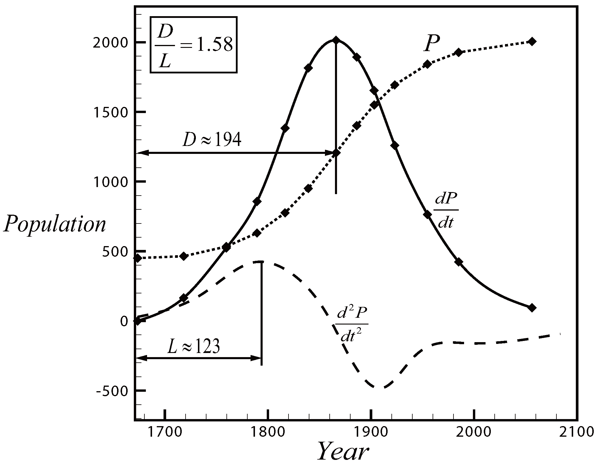
3.4. Population Growth

Though the population of the world does not itself follow the lognormal function, the growth rate nearly follows it, as can be seen from Figure 7 based on the data from Raymond [28]. The population of the world started to grow at an increasing rate since 1650. We see that, for the growth rate, there is an inflexion point (near 1773) and a local maximum point (near 1844). We have thus $D=194$ and $L=123$, and, therefore, $D/L=1.58,$ which is close to the theoretical value.

3.5. Stroke Distribution in Language

Each Chinese word is composed of a number of strokes (while each word of Western languages is composed of a number of letters). The number of words $\left(n_w\right)$ with a specific number $(t=n_s)$ of strokes first increases, reaches a maximum at around $n_s=10$ and decays when $n_s$ further increases.

The function $f_w\left(n_s\right)=n_w\left(n_s\right)$ (number of words) or $f_s\left(n_s\right)=n_s\times n_w\left(n_s\right)$ (total number of strokes for all words with a given $n_s$) approximately follow the lognormal function, as shown in Figure 8, which are obtained using the data from Reference [29]. It is seen that the change of the number of strokes $f_s$ from $n_s=7$ to 8 is the largest, meaning that this is the inflexion point and hence $L=7.5$. The maximum number of $f_s$ occurs at $n_s=12$, hence $D=12$. As a result, $D/L=1.6$. Moreover, $f_s\left(7.5\right)=(910+1312)/2=1111$ and $f_s\left(12\right)=2304$ so that $f_s\left(D\right)/f_s\left(L\right)=2.08$. Both $D/L$ and $f_s\left(D\right)/f_s\left(L\right)$ are close to the ratios shown in Equation (11).

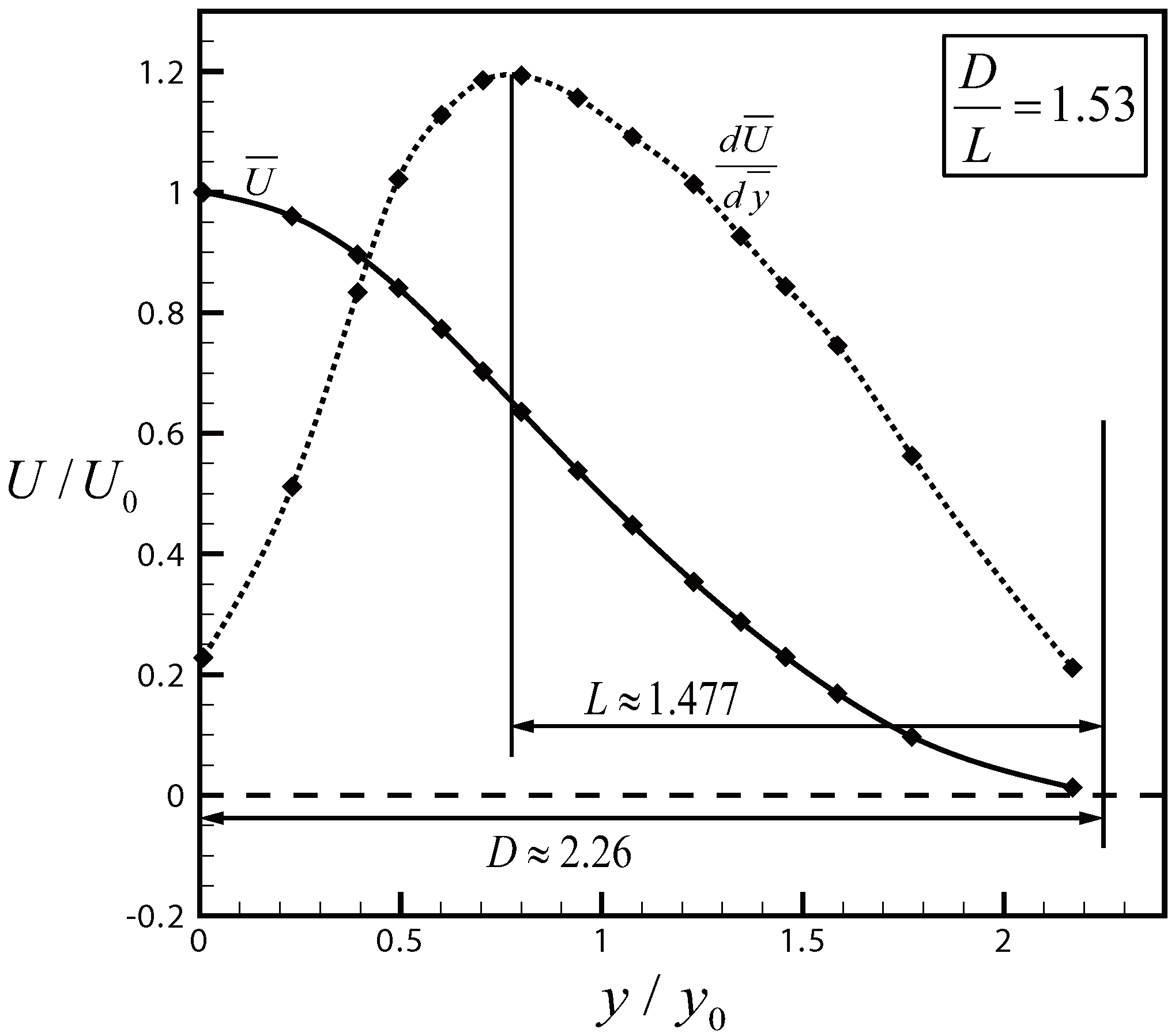
3.6. Possible Significance for Turbulent Flow

First, consider the turbulent free jet. Using a number of experimental data, Rodi [30] gave a fitted curve for the mean axial velocity profile $U/U_0=f(y/y_0)$, where $U_0$ is the velocity on the center line of the jet and y is the radial distance to the center of the jet ($y_0$ is the radial position at which $U=\frac{1}{2}{U}_0$). Figure 9 displays this velocity profile and its derivative with respect to y. We remark that this velocity profile also follows lognormal distribution approximately, and, counting from the outer edge of the jet, which is just $y=2.26y_0$ according to Rodi, the inflexion point is at $L=1.477$, and the maximum (center of the jet) is at $D\approx 2.26$. Hence,

$$\frac{D}{L}=1.53,$$

which is close to the ratio shown in Equation (11).

Consider now the gradient of the velocity, as displayed in Figure 10. We observe that the gradient also has an inflexion point ($L=0.28$, counting from the center of the jet) and a maximum point ($D=0.77$, also counting from the center of the jet) and $D/L\approx 2.75$. This means that, for the velocity gradient, the dissipation is weak so that σ is large and the ratio $D/L$ cannot be predicted.

In turbulent flow, kinetic energy is produced and dissipated so that this is also a typical problem of growth with production and decay. Hence, it would be expected that there be some intrinsic relations between the turbulent properties and the minimal slope of Shannon entropy. We thus attempt to raise some open questions. We know that for turbulent boundary layer flow, the velocity profile in the logarithm regime is described by

$$\frac{u}{u_{*}}=\frac{1}{\kappa }ln\frac{u_{*}y}{\nu }+C,$$

where $u_{*}$ is the friction velocity and ν is the viscosity. Here, κ is the Karman constant. Though the specific value of this constant may be problem dependent [31], it is generally accepted that $\kappa \approx 0.41$, which is remarkably close to the constant $\sigma =\sqrt{6}/6\approx 0.408$. Since the logarithm regime is the regime where turbulence production and dissipation is at equilibrium, the Karman constant κ and the constant σ would be physically related or it would be just the same constant. The justification of this in a more rigorous way is left as an open question.

Again for turbulence, the energy spectrum, $E\left(k\right)$ defined such that ${\int }_0^{\infty }Edk=\mathbf{k}$ where k is the wavenumber and $\mathbf{k}$ is the turbulent kinetic energy, looked at the wavenumber space nearly follows lognormal distribution, especially for isotropic turbulence of large Reynolds number flow [32]. Lower wavenumber corresponds to large eddies coming from production and high wavenumber corresponds to small eddies that are going to be quickly dissipated. Between the energy-containing (for which E has its peak value) and dissipation range, there is a subrange in which $E\left(k\right)\sim k^{-p}$, where $p=5/3$ is the famous Kolmogorov scaling parameter [33]. Whether the two numbers $5/3\simeq 1.6667$ and $\sqrt{e}\simeq 1.6487$ are intrinsically related is the second question open to further studies.

4. Conclusions

We consider in this paper the growth process with a size described by the lognormal function. This size function contains a scale parameter (σ, some measure of the standard deviation) which is normally considered as a free parameter. The slope of the Shannon entropy, obtained by taking the derivative of this entropy to σ, is shown here to have a minimal value at $\sigma =\sqrt{6}/6$. With this free parameter thus uniquely defined, the relations between the inflexion point and maximum point of the lognormal function are also uniquely defined, notably by the base of natural logarithm ($e\simeq 2.718$). In these relations, the location (D) of the maximum is connected to the location (L) of the inflexion point by $D/L=e^{\frac{1}{2}}$ and the sizes are connected by $f_D/f_L=e^{\frac{3}{4}}$.

These relations are useful if the data at the inflexion point are known in advance and the data at the maximum require being predicted. The test using a number of quite different examples shows that these relations have some acceptable accuracy. Thus, the present method of minimizing the Shannon entropy slope is applicable to problems when no other means actually exist for determining the free parameter σ.

The value $\sigma =0.408,$or $\sigma =\sqrt{6}/6,$ has been previously used in References [9,21] for droplet size spreading and epidemic spreading. However, in References [9,21], it was assumed that this follows from the principle of maximum entropy production. Here, we have shown that this value of σ corresponds to minimization of the slope of the Shannon entropy with respect to σ. It is not clear whether this slope minimization is connected to the well-known principle of maximum or minimum entropy production rate [11,12,15,16,34]. Moreover, we have shown in this paper that the relations obtained by the definition of Shannon entropy with $\eta =3$ and the use of the minimization of the Shannon entropy slope have some geometric connection with the minimal surface area or energy principle.

References

1. Barry, B. Patterns of Human Growth, 2nd ed.; Cambridge Studies in Biological and Evolutionary Anthropology; Cambridge University Press: Cambridge, UK, 1999. [Google Scholar]
2. Sutton, J. Gibrat’s Legacy. J. Econ. Lit. 1997, 35, 40–59. [Google Scholar]
3. Daley, D.J.; Gani, J. Epidemic Modeling: An Introduction; Cambridge University Press: Cambridge, UK, 2005. [Google Scholar]
4. Davidson, P.A. Turbulence—An Introduction for Scientists and Engineers; Oxford University Press: Oxford, UK, 2004. [Google Scholar]
5. Stow, C.D.; Stainer, R.D. The physical products of a splashing water drop. J. Meteorol. Soc. Jpn. 1977, 55, 518–532. [Google Scholar]
6. Hohler, S. A law of growth: the logistic curve and population control since world wall II. In Proceedings of the International Conference Technological and Aesthetic (Trans) formation of Society, Darmstadt, Germany, 12–14 October 2005.
7. Gaddum, J.H. Log normal distributions. Nature 1945, 156, 463–466. [Google Scholar] [CrossRef]
8. Limpert, E.; Stahel, W.; Abbt, M. Log-normal distributions across the sciences: Keys and clues. BioScience 2001, 51, 341–352. [Google Scholar] [CrossRef]
9. Wu, Z.N. Prediction of the size distribution of secondary ejected droplets by crown splashing of droplets impinging on a solid wall. Probab. Eng. Mech. 2003, 18, 241–249. [Google Scholar] [CrossRef]
10. Ziegler, H. An Introduction to Thermomechanics; North Holland Publishing: Amsterdam, The Netherlands, 1983. [Google Scholar]
11. Ziegler, H.; Wehrli, C. On a principle of maximal rate of entropy production. J. NonEquilib. Thermodyn. 1987, 12, 229–243. [Google Scholar] [CrossRef]
12. Martyushev, L.M.; Seleznev, V.D. The restrictions of the maximum entropy production principle. Physica A 2014, 410, 17–21. [Google Scholar] [CrossRef]
13. Ozawa, H.; Ohmura, A.; Lorenz, R.D.; Pujol, T. The second law of thermodynamics and the global climate system: A review of the maximum entropy production principle. Rev. Geophys. 2003, 41, 1018–1042. [Google Scholar] [CrossRef]
14. Martyushev, L.M.; Seleznev, V.D. Maximum entropy production principle in physics, chemistry and biology. Phys. Rep. 2006, 426, 1–45. [Google Scholar] [CrossRef]
15. Martyushev, L.M. The maximum entropy production principle: Two basic questions. Philos. Trans. R. Soc. B 2010, 365, 1333–1334. [Google Scholar] [CrossRef] [PubMed]
16. Martyushev, L.M. Entropy and Entropy Production: Old Misconceptions and New Breakthroughs. Entropy 2013, 15, 1152–1170. [Google Scholar] [CrossRef]
17. Ross, J.; Corlan, A.D.; Muler, S.C. Proposed Principle of Maximum Local Entropy Production. J. Phys. Chem. B 2012, 116, 7858–7865. [Google Scholar] [CrossRef] [PubMed]
18. Moreira, A.L.N.; Moita, A.S.; Panao, M.R. Advances and challenges in explaining fuel sprayimpingement: How much of single droplet impact research is useful? Prog. Energy Combust. Sci. 2010, 36, 554–580. [Google Scholar] [CrossRef]
19. Samenfink, W.; Elsaper, A.; Dullenkopf, K.; Wittig, S. Droplet interaction withshear-driven liquid films: Analysis of deposition and secondary droplet characteristics. Int. J. Heat Fluid Flow 1999, 20, 462–469. [Google Scholar] [CrossRef]
20. Schmehl, R.; Rosskamp, H.; Willmann, M.; Wittig, S. CFD analysis of spray propagation and evaporation including wall film formation and spray/film interactions. Int. J. Heat Fluid Flow 1999, 20, 520–529. [Google Scholar] [CrossRef]
21. Wang, W.B.; Wang, C.F.; Wu, Z.N.; Hu, R.F. Modelling the spreading rate of controlled communicable epidemics through an entropy-based thermodynamic model. Sci. China Phys. Mech. 2013, 56, 2143–2150. [Google Scholar] [CrossRef]
22. Dumouchel, C. A new formulation of the Maximum Entropy formalism to model liquid spray drop-size distribution. Part. Part. Syst. Charact. 2006, 23, 469–479. [Google Scholar] [CrossRef]
23. Lucia, U. Stationary open systems: A brief review on contemporary theories on irreversibility. Physica A 2013, 392, 1051–1062. [Google Scholar] [CrossRef]
24. Luchko, Y. Entropy production rate of a one-dimensional alpha-fractional diffusion process. Axioms 2016, 5, 6. [Google Scholar] [CrossRef]
25. Sibulkin, M. A note on the bathtub vortex. J. Fluid Mech. 1962, 14, 21–24. [Google Scholar] [CrossRef]
26. Trefethen, L.M.; Bilger, R.W.; Fink, R.T.; Luxton, R.E.; Tanner, R.T. The bathtub vortex in the Southern Hemisphere. Nature 1965, 207, 1084–1085. [Google Scholar] [CrossRef]
27. Chen, Y.C.; Huang, S.L.; Li, Z.Y.; Chang, C.C.; Chu, C.C. A bathtub vortex under the influence of a protruding cylinder in a rotating tank. J. Fluid Mech. 2013, 733, 134–157. [Google Scholar] [CrossRef]
28. Raymond, P.; Author, T. The Biology of Population Growth; Alfred A. Knopf: New York, NY, USA, 1925. [Google Scholar]
29. Statistics of strokes for the most used chinese characters. J. Lang. Innov. 1958, 3. (In Chinese) [CrossRef]
30. Rodi, W. A review of experimental data of uniform density free turbulent boundary layers. In Studies in Convection I; Launder, B.E., Ed.; Academic Press: London, UK, 1975. [Google Scholar]
31. Trinh, K.T. On the Karman constant. arxiv 2014. [Google Scholar]
32. Landahl, M.T.; Mollo-Christensen, E. Turbulence and Random Processes in Fluid Mechanics; Cambridge University Press: Cambridge, UK, 1986. [Google Scholar]
33. Frisch, U. Turbulence: The Legacy of A. N. Kolmogorov; Cambridge University Press: Cambridge, UK, 1995. [Google Scholar]
34. Polettini, M. Fact-Checking Ziegler’s Maximum Entropy Production Principle beyond the Linear Regime and towards Steady States. Entropy 2013, 15, 2570–2584. [Google Scholar] [CrossRef]
Figure 1. The lognormal function and its derivative. The inflexion point (IP) is at t = t L and the maximum point (MP) is at t = t D .
Entropy 19 00056 g001
Figure 2. The curves of S ( σ ) (with t D = 1 ) and S σ .
Entropy 19 00056 g002
Figure 3. The curves of ϕ σ and ψ σ .
Entropy 19 00056 g003
Figure 4. Angular displacement of the floating disk for a bathtub vortex with reserval, original data from Figure 2 of Sibulkin [17].
Entropy 19 00056 g004
Figure 5. Rotation speed of the floating disk for a bathtub vortex with reserval, original data from Figure 2 of Sibulkin [17].
Entropy 19 00056 g005
Figure 6. Droplet size distribution for one set of data of Stow and Stainer [5].
Entropy 19 00056 g006
Figure 7. Population growth in the world.
Entropy 19 00056 g007
Figure 8. Traditional Chinese words and total strokes.
Entropy 19 00056 g008
Figure 9. Velocity profile in a turbulent jet.
Entropy 19 00056 g009
Figure 10. Velocity gradient profile in a turbulent jet.
Entropy 19 00056 g010