
Bateman–Feshbach Tikochinsky and Caldirola–Kanai Oscillators with New Fractional Differentiation

 , , ,
, , , 
Abstract
:1. Introduction
2. Fractional Operators
3. Applications
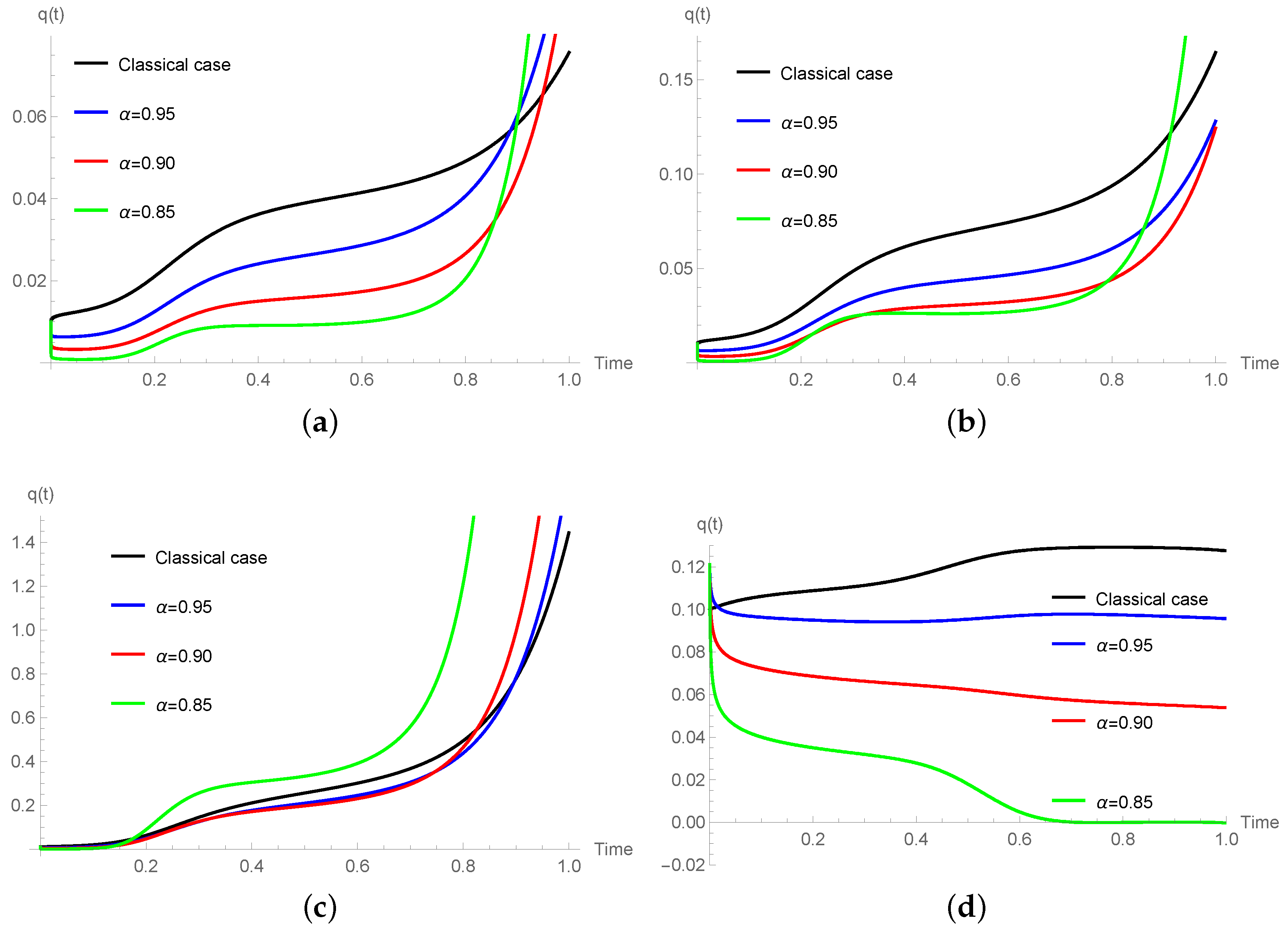
3.1. Bateman–Feshbach–Tikochinsky Oscillator
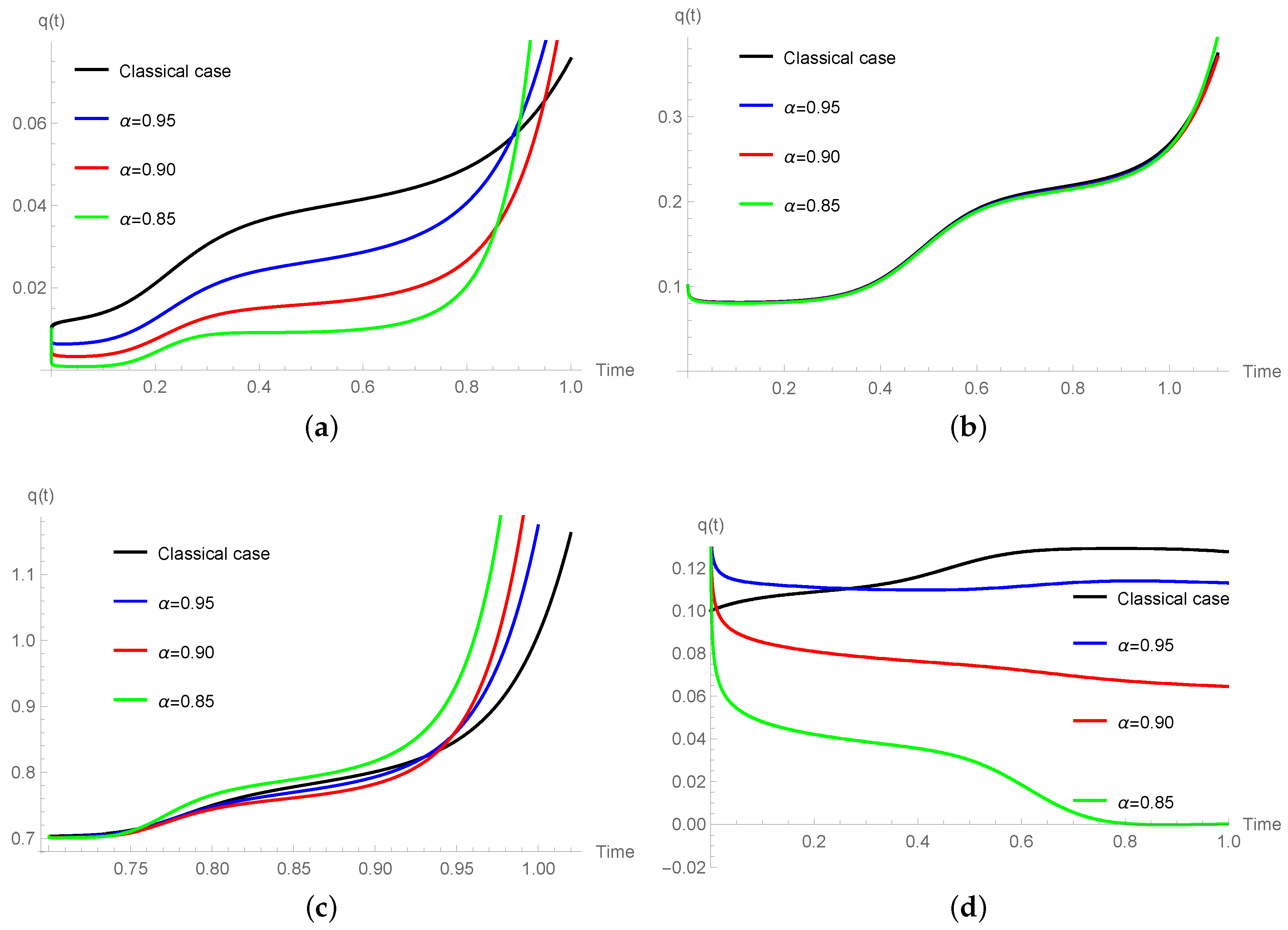
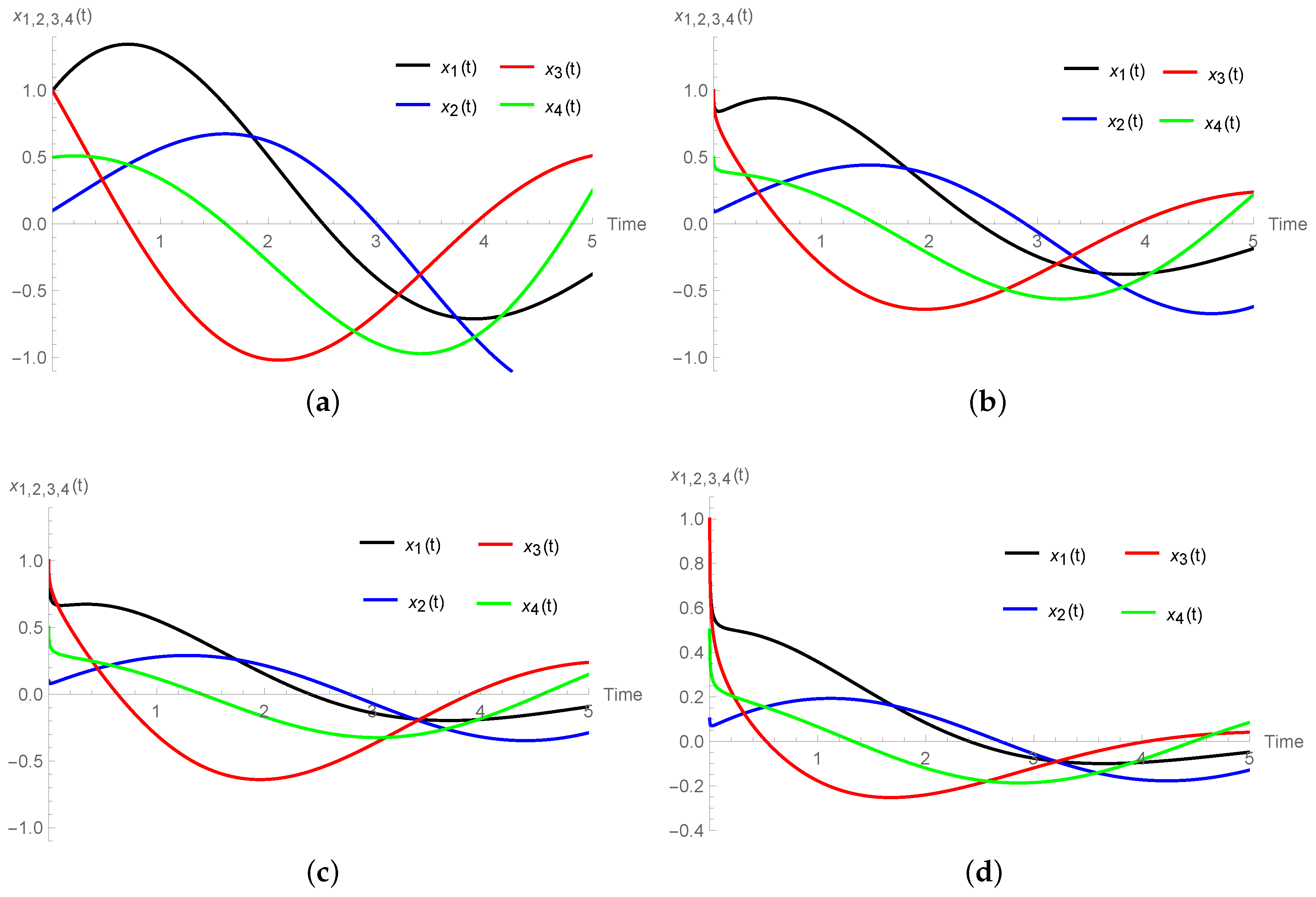
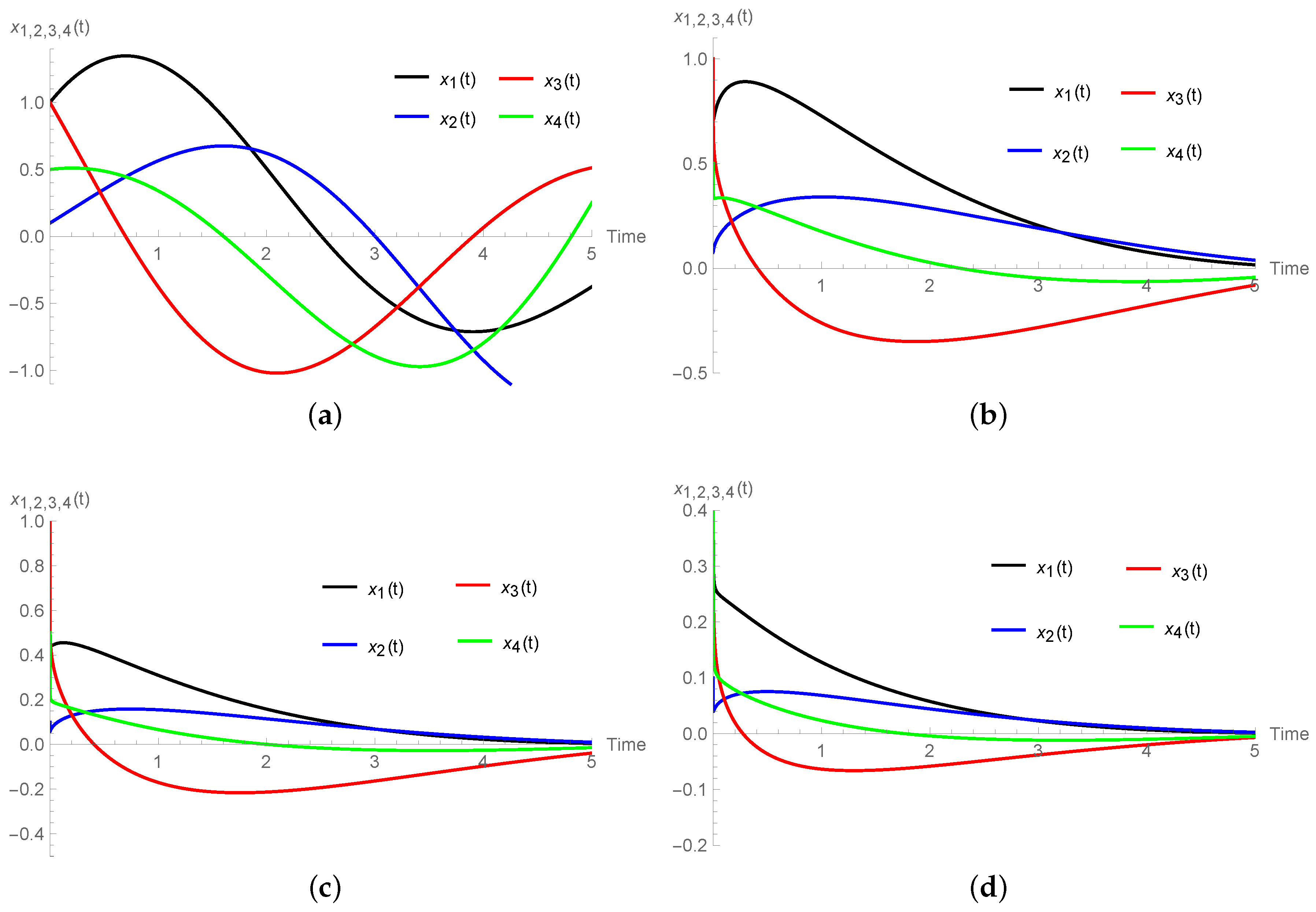
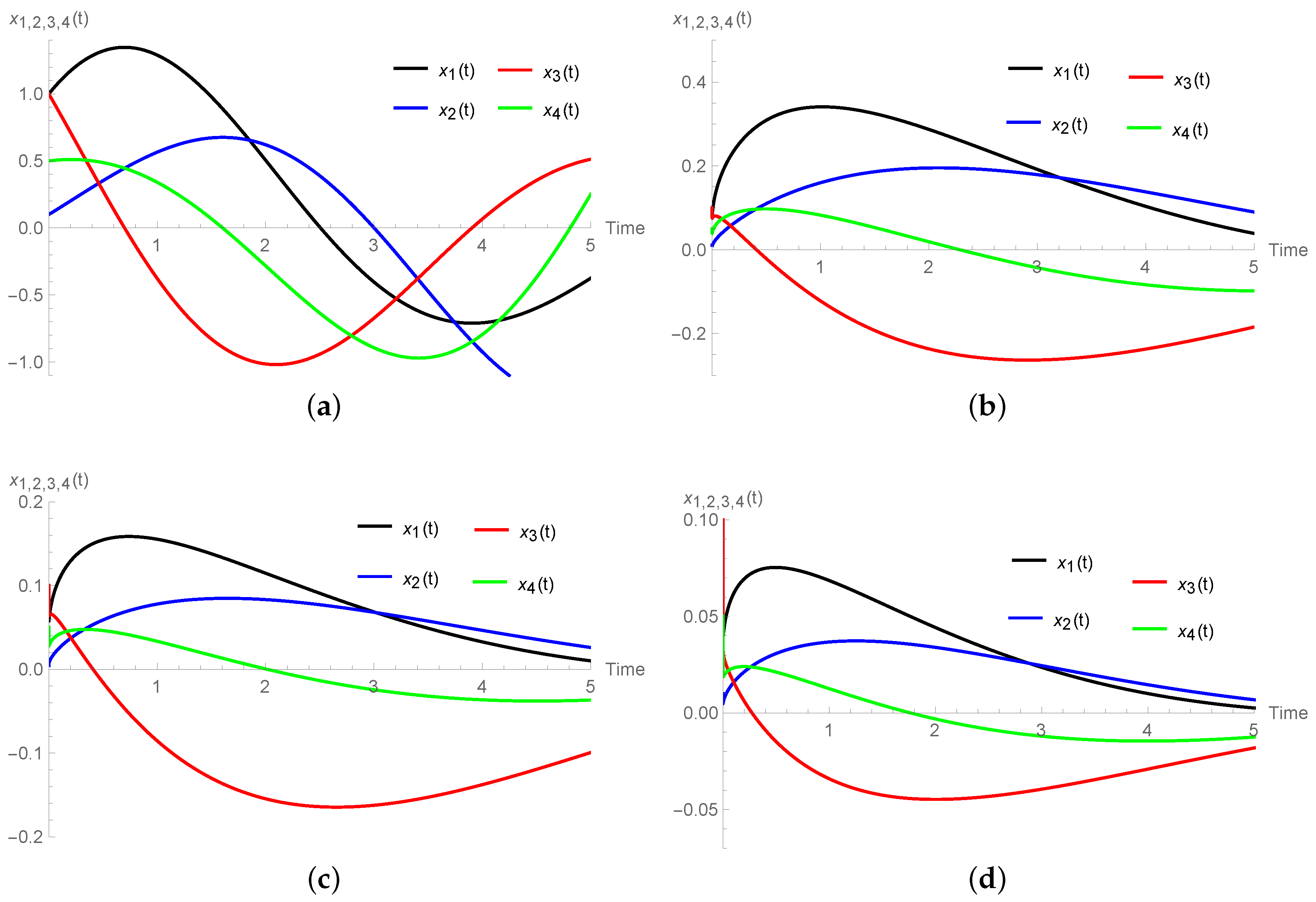
Numerical Simulations
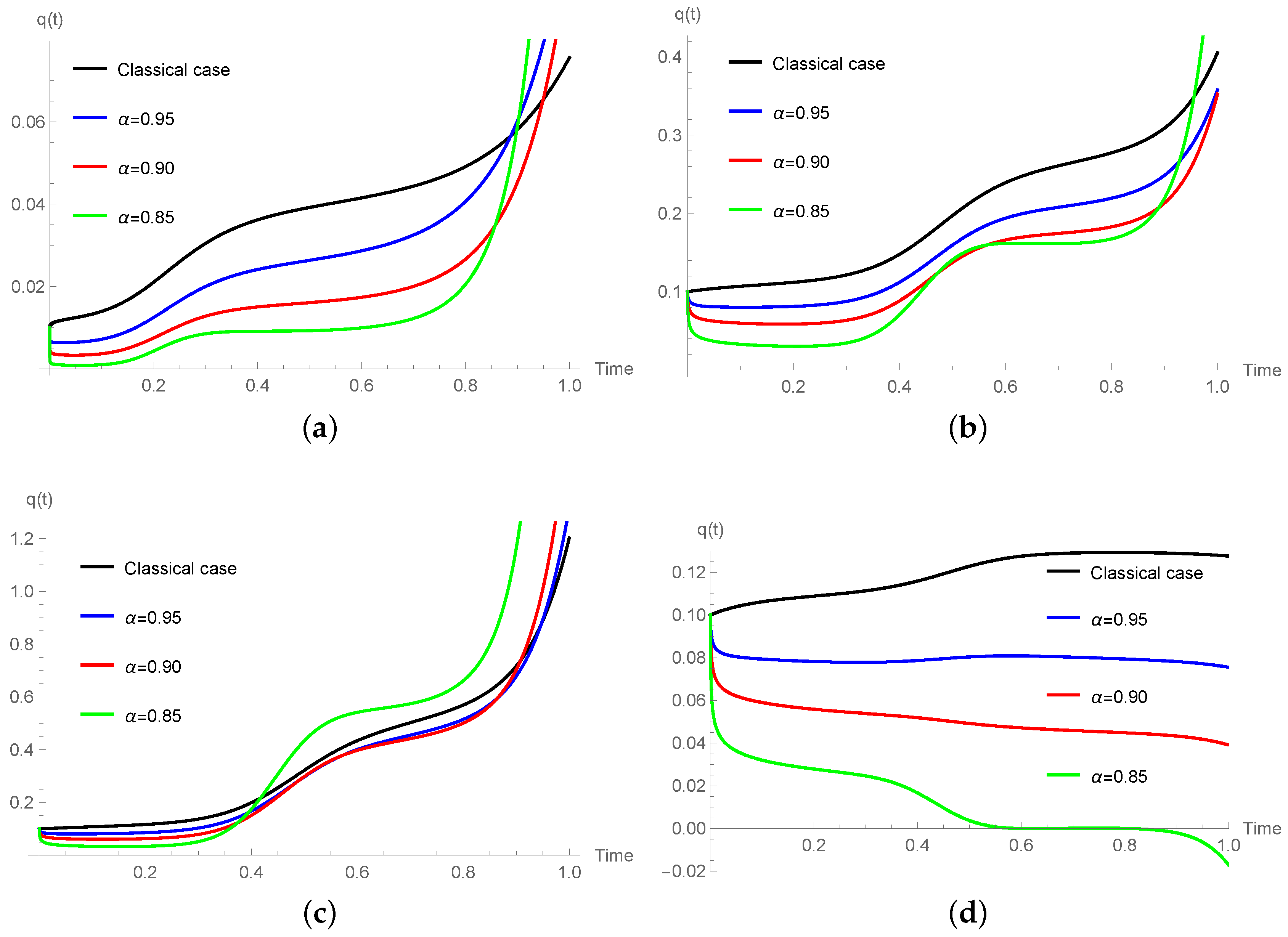
3.2. Caldirola–Kanai Oscillator
Numerical Simulations
4. Conclusions
Acknowledgments
Author Contributions
Conflicts of Interest
References
- Kim, S.P.; Santana, A.E.; Khanna, F.C.; Kor, J. Decoherence of quantum damped oscillators. Phys. Soc. 2003, 43, 452–460. [Google Scholar]
- Bateman, H. On dissipative systems and related variational principles. Phys. Rev. 1931, 38. [Google Scholar] [CrossRef]
- Feshbach, H.; Tikochinsky, Y. Quantization of the damped harmonic oscillator. Trans. N. Y. Acad. Sci. 1977, 38, 44–53. [Google Scholar] [CrossRef]
- Caldirola, P. Forze non conservative nella meccanica quantistica. Il Nuovo Cimento 1942, 18, 393–400. (In Italian) [Google Scholar] [CrossRef]
- Kanai, E. On the quantization of the dissipative systems. Prog. Theor. Phys. 1948, 3, 440–442. [Google Scholar] [CrossRef]
- Dekker, H. Classical and quantum mechanics of the damped harmonic oscillator. Phys. Rep. 1981, 80. [Google Scholar] [CrossRef]
- Baleanu, D.; Asad, J.H.; Petras, I. Fractional Bateman–Feshbach Tikochinsky Oscillator. Commun. Theor. Phys. 2014, 61, 221–225. [Google Scholar] [CrossRef]
- Baleanu, D.; Asad, J.H.; Petras, I.; Elagan, S.; Bilgen, A. Fractional Euler-Lagrange equation of Caldirola–Kanai oscillator. Rom. Rep. Phys. 2012, 64, 1171–1177. [Google Scholar]
- Atangana, A.; Alkahtani, B.S.T. Analysis of the Keller-Segel model with a fractional derivative without singular kernel. Entropy 2015, 17, 4439–4453. [Google Scholar] [CrossRef]
- Caputo, M.; Fabricio, M. A New Definition of Fractional Derivative without Singular Kernel. Prog. Fract. Differ. Appl. 2015, 1, 73–85. [Google Scholar]
- Caputo, M.; Fabrizio, M. Applications of new time and spatial fractional derivatives with exponential kernels. Prog. Fract. Differ. Appl. 2016, 2. [Google Scholar] [CrossRef]
- Batarfi, H.; Losada, J.; Nieto, J.J.; Shammakh, W. Three-point boundary value problems for conformable fractional differential equations. J. Funct. Spaces 2015, 2015. [Google Scholar] [CrossRef]
- Sitho, S.; Ntouyas, S.K.; Tariboon, J. Existence results for hybrid fractional integro-differential equations. Bound. Value Probl. 2015, 2015. [Google Scholar] [CrossRef]
- Gao, F.; Yang, X.J. Fractional Maxwell fluid with fractional derivative without singular kernel. Therm. Sci. 2016, 20, 871–877. [Google Scholar] [CrossRef]
- Shah, N.A.; Khan, I. Heat transfer analysis in a second grade fluid over and oscillating vertical plate using fractional Caputo Fabrizio derivatives. Eur. Phys. J. C 2016, 76. [Google Scholar] [CrossRef]
- Caputo, M.; Cametti, C. Fractional derivatives in the transport of drugs across biological materials and human skin. Phys. A Stat. Mech. Its Appl. 2016, 462, 705–713. [Google Scholar] [CrossRef]
- Gómez-Aguilar, J.F. Modeling diffusive transport with a fractional derivative without singular kernel. Phys. A Stat. Mech. Its Appl. 2016, 447, 467–481. [Google Scholar] [CrossRef]
- Zafar, A.A.; Fetecau, C. Flow over an infinite plate of a viscous fluid with non-integer order derivative without singular kernel. Alex. Eng. J. 2016, 55, 2789–2796. [Google Scholar] [CrossRef]
- Atangana, A.; Baleanu, D. New fractional derivatives with nonlocal and non-singular kernel: Theory and application to heat transfer model. Therm. Sci. 2016, 20, 763–769. [Google Scholar] [CrossRef]
- Gómez-Aguilar, J.F. Space-time fractional diffusion equation using a derivative with nonsingular and regular kernel. Phys. A Stat. Mech. Its Appl. 2017, 465, 562–572. [Google Scholar] [CrossRef]
- Gómez-Aguilar, J.F. Irving Mullineux oscillator via fractional derivatives with Mittag–Leffler kernel. Chaos Solitons Fractals 2017, 95, 179–186. [Google Scholar] [CrossRef]
- Atangana, A.; Koca, I. Chaos in a simple nonlinear system with Atangana-Baleanu derivatives with fractional order. Chaos Solitons Fractals 2016, 89, 447–454. [Google Scholar] [CrossRef]
- Changpin, L.; Chunxing, T. On the fractional Adams method. Comput. Math. Appl. 2009, 58, 1573–1588. [Google Scholar]
- Diethelm, K.; Ford, N.J.; Freed, A.D. Detailed error analysis for a fractional Adams method. Numer. Algorithms 2004, 36, 31–52. [Google Scholar] [CrossRef]
- Baskonus, H.M.; Bulut, H. On the numerical solutions of some fractional ordinary differential equations by fractional Adams-Bashforth-Moulton method. Open Math. 2015, 13, 547–556. [Google Scholar] [CrossRef]
- Changpin, L.; Guojun, P. Chaos in Chen’s system with a fractional order. Chaos Solitons Fractals 2004, 22, 443–450. [Google Scholar]

© 2017 by the authors. Licensee MDPI, Basel, Switzerland. This article is an open access article distributed under the terms and conditions of the Creative Commons Attribution (CC BY) license ( http://creativecommons.org/licenses/by/4.0/).
Share and Cite
Coronel-Escamilla, A.; Gómez-Aguilar, J.F.; Baleanu, D.; Córdova-Fraga, T.; Escobar-Jiménez, R.F.; Olivares-Peregrino, V.H.; Qurashi, M.M.A. Bateman–Feshbach Tikochinsky and Caldirola–Kanai Oscillators with New Fractional Differentiation. Entropy 2017, 19, 55. https://doi.org/10.3390/e19020055
Coronel-Escamilla A, Gómez-Aguilar JF, Baleanu D, Córdova-Fraga T, Escobar-Jiménez RF, Olivares-Peregrino VH, Qurashi MMA. Bateman–Feshbach Tikochinsky and Caldirola–Kanai Oscillators with New Fractional Differentiation. Entropy. 2017; 19(2):55. https://doi.org/10.3390/e19020055
Chicago/Turabian StyleCoronel-Escamilla, Antonio, José Francisco Gómez-Aguilar, Dumitru Baleanu, Teodoro Córdova-Fraga, Ricardo Fabricio Escobar-Jiménez, Victor H. Olivares-Peregrino, and Maysaa Mohamed Al Qurashi. 2017. "Bateman–Feshbach Tikochinsky and Caldirola–Kanai Oscillators with New Fractional Differentiation" Entropy 19, no. 2: 55. https://doi.org/10.3390/e19020055