Label-Driven Learning Framework: Towards More Accurate Bayesian Network Classifiers through Discrimination of High-Confidence Labels


1
College of Computer Science and Technology, Jilin University, Changchun 130012, China
2
Key Laboratory of Symbolic Computation and Knowledge Engineering of Ministry of Education, Jilin University, Changchun 130012, China
*
Authors to whom correspondence should be addressed.
Entropy 2017, 19(12), 661; https://doi.org/10.3390/e19120661
Submission received: 31 October 2017
/
Revised: 26 November 2017
/
Accepted: 30 November 2017
/
Published: 3 December 2017
(This article belongs to the Special Issue Symbolic Entropy Analysis and Its Applications)
Abstract
:Bayesian network classifiers (BNCs) have demonstrated competitive classification accuracy in a variety of real-world applications. However, it is error-prone for BNCs to discriminate among high-confidence labels. To address this issue, we propose the label-driven learning framework, which incorporates instance-based learning and ensemble learning. For each testing instance, high-confidence labels are first selected by a generalist classifier, e.g., the tree-augmented naive Bayes (TAN) classifier. Then, by focusing on these labels, conditional mutual information is redefined to more precisely measure mutual dependence between attributes, thus leading to a refined generalist with a more reasonable network structure. To enable finer discrimination, an expert classifier is tailored for each high-confidence label. Finally, the predictions of the refined generalist and the experts are aggregated. We extend TAN to LTAN (Label-driven TAN) by applying the proposed framework. Extensive experimental results demonstrate that LTAN delivers superior classification accuracy to not only several state-of-the-art single-structure BNCs but also some established ensemble BNCs at the expense of reasonable computation overhead.
1. Introduction
Supervised classification is a fundamental issue in machine learning and data mining. The task of supervised classification can be described as given a labelled training set with t training instances, predicting a class label for a testing instance x (), where is the value of an attribute and is a value of the class variable C. Among numerous classification techniques, Bayesian network classifiers (BNCs) are well-known for their model interpretability, comparable classification performance and the ability to directly handle multi-class classification problems [1]. A BNC provides a confidence measure in the form of a posterior probability for each class label and performs a classification by assigning the label with the maximum posterior probability to x, that is:
By learning a more reasonable network structure, a BNC can often achieve higher classification accuracy. Naive Bayes (NB) assumes all the attributes are independent given the class. When dealing with large datasets with complex attribute dependencies, its performance degrades dramatically. To mine significant attribute dependencies in training data, the tree-augmented naive Bayes (TAN) classifier [2] models 1-dependence relations between attributes by building a maximal weighted spanning tree. The k-dependence Bayesian classifier (KDB) [3] allows us to construct classifiers at arbitrary points along the attribute dependence spectrum by varying the value of k. To explore possible attribute dependencies that exist in testing data, instance-based BNCs [4] learn the most appropriate network structure for each testing instance at classification time. The local KDB (LKDB) [5] captures local dependence relations between attributes. The lazy subsumption resolution [6] identifies occurrences of the specialization-generalization relationship and eliminates generalizations at classification time. By combining predictions from multiple BNCs, ensemble learning can help to achieve better overall accuracy, on average, than any individual member. The averaged one-dependence estimators (AODE) [7] learns a restricted class of one-dependence estimators. The weighted averaged TAN (WATAN) [8] constructs a set of TANs by choosing each attribute as the root of the tree and uses the mutual information between the root attribute and the class variable as the aggregation weight. The averaged KDB (AKDB) [5] is an ensemble of KDB and LKDB.
From the viewpoint of entropy, the uncertainty of a prediction will be highest when all estimated posterior probabilities are equiprobable. It can thus be inferred that BNCs are prone to making a wrong prediction when some labels bear high confidence degrees (or posterior probabilities) close to that of the predicted label. We propose to improve classification accuracy of BNCs by alleviating this problem. To the best of our knowledge, it has not previously been explored. To further discriminate among high-confidence labels, we resort to multistage classification. Multistage classification is characterized by the property that a prediction is made using a sequence of classifiers that operate in cascade [9]. It has been widely applied in many domains of pattern recognition, such as character recognition [10], age estimation [11] and face recognition [12]. The multistage classification methodology proposed in [13] aims at reducing mutual misclassifications among easily confused labels and consists of two stages. Firstly, an inexpensive classifier, which can discriminate among all labels, coarsely classifies a testing instance. If the predicted label has some labels that tend to be confused with it (denoted as ), the testing instance will be fed to a localized and more sophisticated classifier which concentrates on , thus obtaining a refined prediction.
Following the learning paradigm proposed in [13], we devise the label-driven learning framework, where instance-based learning and ensemble learning work in concert. To deal with the potential misclassification problem of BNCs, the framework learns three models, each built in a different stage. In the preprocessing stage, a generalist classifier carries out a first classification to obtain high-confidence labels. If there exists more than one such label, the testing instance will be reconsidered in following two stages. In the label filtering stage, by exploiting credible information derived from high-confidence labels, a refined generalist with a more accurate network structure is deduced for each reconsidered testing instance. Innovatively, we add an extra hierarchy level to the structure proposed in [13] by increasing the degree of localisation. In the label specialization stage, a Bayesian multinet classifier (BMC) is built to model label-specific causal relationships in the context of a particular reconsidered testing instance. Each local network of the BMC is an expert classifier, which targets a specific high-confidence label. Finally, rather than relying on the decision of a single classifier, the framework averages the predictions of the refined generalist and the experts, which possesses the merits of ensemble learning.
TAN has demonstrated satisfactory classification accuracy, while maintaining efficiency and simplicity. Hence, as a first attempt, we apply the proposed label-driven learning framework to TAN and name the resulting model LTAN (Label-driven TAN). Through extensive experiments on 40 datasets from the UCI (University of California, Irvine) machine learning repository [14], we prove that the proposed framework can alleviate the potential misclassification problem of TAN without causing too many offsetting errors or incurring very high computation overhead. Empirical comparisons also reveal that LTAN outperforms several state-of-the-art single-structure BNCs (NB, TAN and KDB), as well as three established ensemble BNCs (AODE, WATAN and AKDB) in terms of classification accuracy.
The remainder of the paper is organized as follows: Section 2 provides a short background to information theory and reviews the related BNCs and BMC. In Section 3, we describe our label-driven learning framework in detail. The extensive empirical results of the proposed framework are presented in Section 4. In Section 5, we analyze why LTAN degrades the classification accuracy of TAN on a few datasets. To summarize, Section 6 shows the main conclusions and outlines future work.
2. Preliminaries
2.1. Information Theory
Although information theory was primarily concerned with the problem of digital communication when it was first introduced by Claude E. Shannon in the 1940s [15], the theory has much broader applicability in the field of classification [16,17]. Here, we review several commonly used definitions. In the following discussion, upper-case letters denote random variables (attributes or the class variable in the context of classification), lower-case letters denote specific values taken by corresponding variables, and the set of all possible values of a random variable, say X, is represented by .
Definition 1 ([18]).
The entropy of X measures its unpredictability. It is defined as:
Definition 2 ([18]).
Conditional entropy measures the amount of information needed to describe X when the value of Y is known. It is defined as:
Definition 3 ([18]).
Mutual information () measures how much information X bears on Y. More specifically, it quantifies the reduction of the entropy of X after observing the value of Y. It is defined as:
Definition 4 ([18]).
Conditional mutual information () measures the information that X provides about Y given the value of a third variable Z. It is defined as:
2.2. Bayesian Network Classifiers
A Bayesian network (BN) can be formalized as a pair [19]. The structure is a directed acyclic graph, where vertices correspond to the class variable or attributes and edges represent dependencies between child nodes and their parent nodes. The parameter set contains a conditional probability distribution for each vertex in , namely or , where is the set of values of the attributes that are parents of node in structure and the same applies for c. In our present work, the class variable does not have any parents, so we have . Thus, a BN defines a joint probability distribution as:
Taking advantage of the underlying BN , a BNC computes in Equation (1) by
In practice, the conditional probability distributions in are stored in conditional probability tables (s), which are obtained from the training set .
2.2.1. Naive Bayes
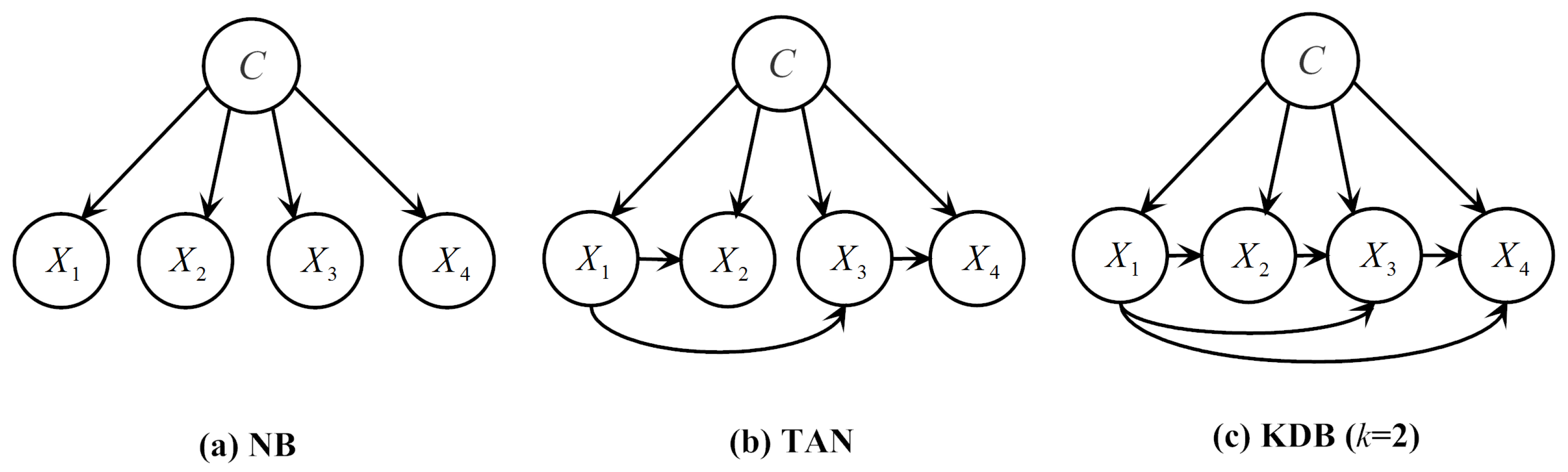
Unfortunately, it has been proved that learning an optimal BN is NP-hard [20]. One practical approach to dealing with the intractable complexity is to learn a constrained or totally pre-fixed network structure. The simplest of these structures is the one used by NB. NB assumes all the attributes are independent given the class variable (see Figure 1a). Consequently, NB calculates using the following formula:
As indicated in Section 1, the attribute independence assumption of NB is often violated in the real world, which may deteriorate its classification performance.
2.2.2. TAN and WATAN
One extension of NB is TAN, which relaxes the independence assumption of NB. TAN imposes a tree structure on NB, where each attribute has the class variable and one other attribute as its parents, except a single attribute, which has only the class variable as its parent and is the root of the tree (see Figure 1b). TAN uses between two attributes given the class variable to construct the maximum likelihood tree by finding a maximal weighted spanning tree (MST) in a graph. Prim’s algorithm [21], which is one of the most popular MST searching algorithms, is selected in our current work for its low time complexity and easy implementation. The learning algorithm of TAN is depicted in Algorithm 1.
ATAN is proposed to enhance the class probability estimation performance of TAN, in terms of conditional log likelihood [8]. In ATAN, all attributes take turns to be the root node, resulting in a set of TANs. To make a prediction, the estimated class-membership probabilities of each built TAN are averaged. ATAN is further improved by using the between the root attribute and the class variable as the aggregation weight. The improved ATAN is referred to as weighted ATAN (WATAN) [8].
| Algorithm 1: The TAN learning algorithm. |
| Input: s. Output: The built TAN model . 1 Let be a matrix of , where , if ; 2 ; // Algorithm 2 3 add the class node C to and add an arc from C to each attribute node; 4 return ; |
| Algorithm 2: treeConstruction(). |
| Input: The edge weight matrix , whose element is denoted as . Output: The built directed MST . 1 Let be a complete undirected graph where vertices are the attributes and the weight of the edge connecting to is annotated by ; 2 ; // perform Prim’s algotithm to find an MST in 3 Transform the resulting undirected tree to a directed tree by choosing a root attribute and setting the direction of all edges to be outward from it.; 4 return ; |
2.2.3. KDB and LKDB
To alleviate the independence assumption of NB, KDB allows each attribute to have at most k attributes as its parents (see Figure 1c). Learning a KDB structure first involves ranking attributes using between an attribute and the class variable. Then, for attribute being placed in position i of the ranking, the k attributes taken from with the highest are set as parents. Finally, the class variable C is added as a parent for all the attributes. Given a certain k, the time complexity of training KDB is [22], where t is the number of training instances and n is the number of attributes.
Dependence relations between attributes may vary from one testing instance to another [5]. The conventional KDB structure can not automatically adapt to different testing instances. To remedy this limitation, LKDB is proposed. To identify dynamic changes of dependence relations between attributes, and are defined in [5] as follows:
Definition 5.
Local mutual information (LMI) is defined to measure the reduction of entropy about the class variable C after observing that , as follows:
Definition 6.
Conditional local mutual information (CLMI) is defined to measure the amount of information shared between two attribute values and given the class variable C, as follows:
Instead of and , LKDB uses for attribute ranking and for parent assignment. At classification time, a LKDB model is built for each testing instance to capture local dependence relations between attributes. Calculating between attributes and the class variable takes time . Computing between every pair of attributes given the class variable is of time complexity . Attribute ranking and parent assignment are and respectively. Hence, classifying a testing instance using LKDB has time complexity . By combining the predictions of the robust KDB model and the flexible LKDB model, the averaged KDB (AKDB) achieves even higher classification performance [5].
2.3. Bayesian Multinet Classifiers
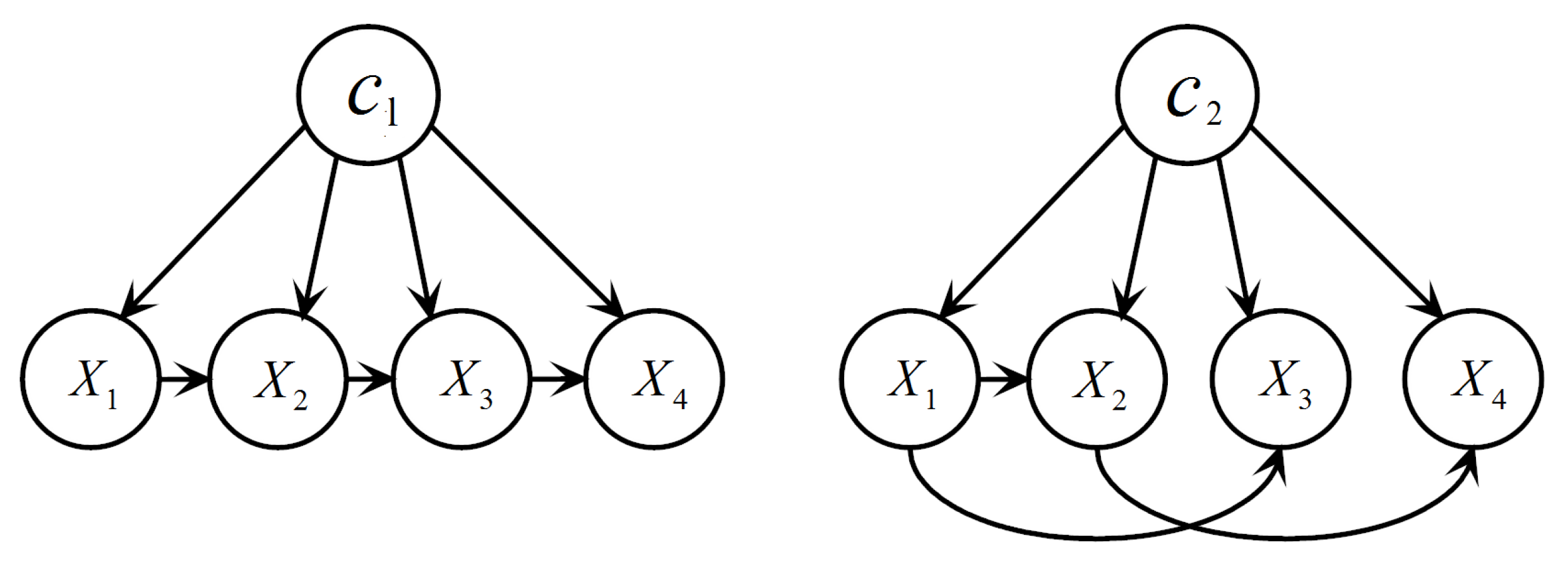
A BN forces dependence relations between attributes to be the same for all labels, thus cannot handle the problem of asymmetric independence, which refers to conditional independence relationships only held for some but not all the values that the class variable takes [23]. Bayesian multinets (BMs) [24] offer a solution. Formally, a BM is a tuple , where is the probability distribution of C, and is the local BN corresponding to label . Conditioned on each label, attributes can form different local BNs with different structures, thereby enabling the representation of asymmetric independence assertions. A BM defines a joint distribution:
where is the set of values of the attributes that are parents of node in the local BN . Consequently, a Bayesian multinet classifier (BMC) classifies a testing instance using:
The Bayesian Chow–Liu tree multinet classifier [25], or BMC for short, is a typical BMC which performs as well as TAN [2]. Figure 2 illustrates a BMC structure. Each local BN of a BMC is a Chow–Liu tree that is built using the procedure proposed by Chow and Liu [26]. The procedure is essentially the same as the one outlined in Algorithm 1 with the exception that in step 1 is replaced by . The procedure is executed separately for each label using the training set , where is the set of training instances labelled in . Note that, since we compute the in each , the label conditional mutual information () is actually computed, which is defined as:
Taking advantage of , Algorithm 3 gives a more efficient implementation of BMC compared with the one in [26], as there is no need to partition the training set.
| Algorithm 3: The BMC learning algorithm. |
 |
3. Label-Driven Learning Framework
3.1. Motivation
As mentioned in Section 1, BNCs (e.g., TAN) are probabilistic classifiers that produce an interpretable confidence value for each class label in the form of a posterior probability. Table 1 presents two examples where TAN is utilized to classify two testing instances in the Nursery dataset. The Nursery dataset is collected from the UCI machine learning repository and has five class labels [14]. The class membership probabilities of the testing instances in Table 1 estimated by TAN are listed in Table 2.
For the first instance, the high posterior probability of (0.9984) provides strong evidence for choosing as the predicted label. The classifier is very confident in this choice and in fact it is a correct one. For the second instance, the posterior probability of (0.4945) is very close to that of (0.5051). The label with the maximum posterior probability is always chosen as the predicted label. According to this rule, although is only slightly greater than by 0.0106, is still chosen to be the predicted label. However, it turns out that is the true label. The reason for this misclassification may be that the small advantage of over has little credibility. In practice, posterior probabilities are hard to be accurately estimated especially when the training data is scarce, so the small advantage of the maximum posterior probability of a testing instance can often only be attributed to chance. Predictions based upon these coincidental advantages are hardly reliable. We can thus infer:
- When posterior probabilities of some class labels are close to the maximum posterior probability, there is a high risk of misclassification.
- When the maximum posterior probability is far greater than the posterior probabilities of other labels, the classification result is more credible—in other words, more likely to be correct.
Here, a criterion to quantify how close the maximum posterior probability is to the posterior probabilities of other labels is desired. A simple and straightforward choice is the ratio between them. Hence, given a testing instance x, the set of labels whose posterior probabilities are close to or equal to the maximum posterior probability can be obtained by:
where is the label predicted by a Bayesian classifier and is a user-specified threshold (). Note that is always included in , so always holds, where is the cardinality of a set.
According to the above two inferences, alerts us that has some strong competitors who are also very likely to be the true label. A hasty decision of directly choosing may be error-prone. To address this problem, we augment the classification process of a BNC with an extra reconsideration process for each testing instance whose includes not only . In this process, labels in are reevaluated using the proposed label-driven learning framework. As for instances whose includes only , we can somewhat trust the decision made by the classifier. Therefore, there is no need to reconsider such instances with the label-driven learning framework.
The proposed label-driven learning framework consists of three stages: preprocessing, label filtering and label specialization. In the preprocessing stage, a conventional BNC is utilized as the generalist to provide initial, coarse predictions. If a testing instance satisfies , the prediction of the generalist (denoted as ) will be accepted; otherwise, it is deemed unreliable and the testing instance will be reconsidered. For reconsidered testing instances for which the generalist fails to make reliable predictions, the latter two stages will come into play to further discriminate among labels in , which are discussed in Section 3.2 and Section 3.3, respectively.
3.2. Label Filtering Stage
As TAN provides a good trade-off between computation complexity and classification accuracy, we choose it as the generalist in this work. The generalist classifier TAN uses the metric to build an MST. From the definition of , we can derive the following equation:
Equation (15) indicates that can be decomposed into two parts: information derived from labels in (if ) and information derived from labels in . Since the posterior probabilities of classes in are quite small, it is almost impossible for the class variable to take the values in . Therefore, the former part of has low confidence and may lead to imprecise measurements of mutual dependence between attributes. In light of this, for each reconsidered testing instance, labels in are first removed, i.e., eliminated from further consideration and then the MST of TAN is reconstructed with information derived from labels in only. in Equation (14) is a crucial threshold to judge whether a label should be filtered out or not. We will perform an empirical study to determine in Section 4.1.
After removing labels in , the label space of a reconsidered testing instance is reduced from to . The remaining part (the latter part) of is formalized as:
Definition 7.
Given a testing instance , a Bayesian network classifier and a user-specified threshold δ (), the reduced conditional mutual information is the CMI between two attributes and given the class variable C, who can take values only from . It can be calculated using:
where can be obtained by
where is the label predicted by .
The label filtering stage reconstructs the MST of TAN using in replacement of as the metric for edge weight computations. By eliminating low-confidence information derived from removed labels, the reconstructed MST can capture the dependence relations between attributes more accurately. Furthermore, as varies from testing instance to testing instance, also changes accordingly. Consequently, each reconsidered testing instance may have a different tree structure that is the most appropriate for it. Compared with the uniform MST structure that TAN builds for all testing instances, the reconstructed MST structure is not only more accurate but also more flexible.
By reconstructing the MST of TAN using the edge weighting scheme, a refined TAN model can be learned, which we call Information Elimination TAN, or TAN for short. TAN serves as a refined generalist. The refined generalist can provide more accurate estimations of posterior probabilities for labels in .
3.3. Label Specialization Stage
Due to the problem of asymmetric independence (introduced in Section 2.3), the refined generalist that learns a single structure is unable to express different dependence relations between attributes when C takes different values. To address this deficiency and further discriminate among labels in , the label specialization stage learns a BMC for each reconsidered testing instance. As mentioned in Section 2.3, BMC achieves classification performance comparable to TAN. Hence, we consider adopting BMC. However, it can not be immediately applied to our current problem. As pointed out in Section 2.2.3, dependence relations between attributes of different testing instances may differ significantly. However, the metric that is adopted by BMC for computing edge weights of local Chow–Liu trees is invariant for all testing instances. Consequently, BMC is unable to adjust its local network structures dynamically to fit different testing instances. Encouraged by the success of and on LKDB, we generalize the definition of to remedy this limitation. The new metric conditional pointwise mutual information () is defined as:
Definition 8.
Conditional pointwise mutual information measures the amount of information shared between two attribute values and conditioned on the label c. can be calculated using:
BMC can be improved by using in replacement of as the edge weighting scheme for local Chow–Liu tree construction. We refer to the improved BMC as instance-based BMC, or IBMC for short.
Each local network of IBMC can be regarded as an expert oriented to a single label in . Let Expert be the local network corresponding to a label . Expert can encode label-specific correlations between attributes, thereby providing an accurate posterior probability estimation for . Eventually, for each label , the posterior probabilities estimated by the refined generalist and the corresponding expert, denoted as ) and ), respectively, are averaged. The label-driven learning framework then assigns the most probable a posteriori (MAP) class (denoted as ) in to a reconsidered testing instance.
3.4. Overall Structure and Complexity Analysis
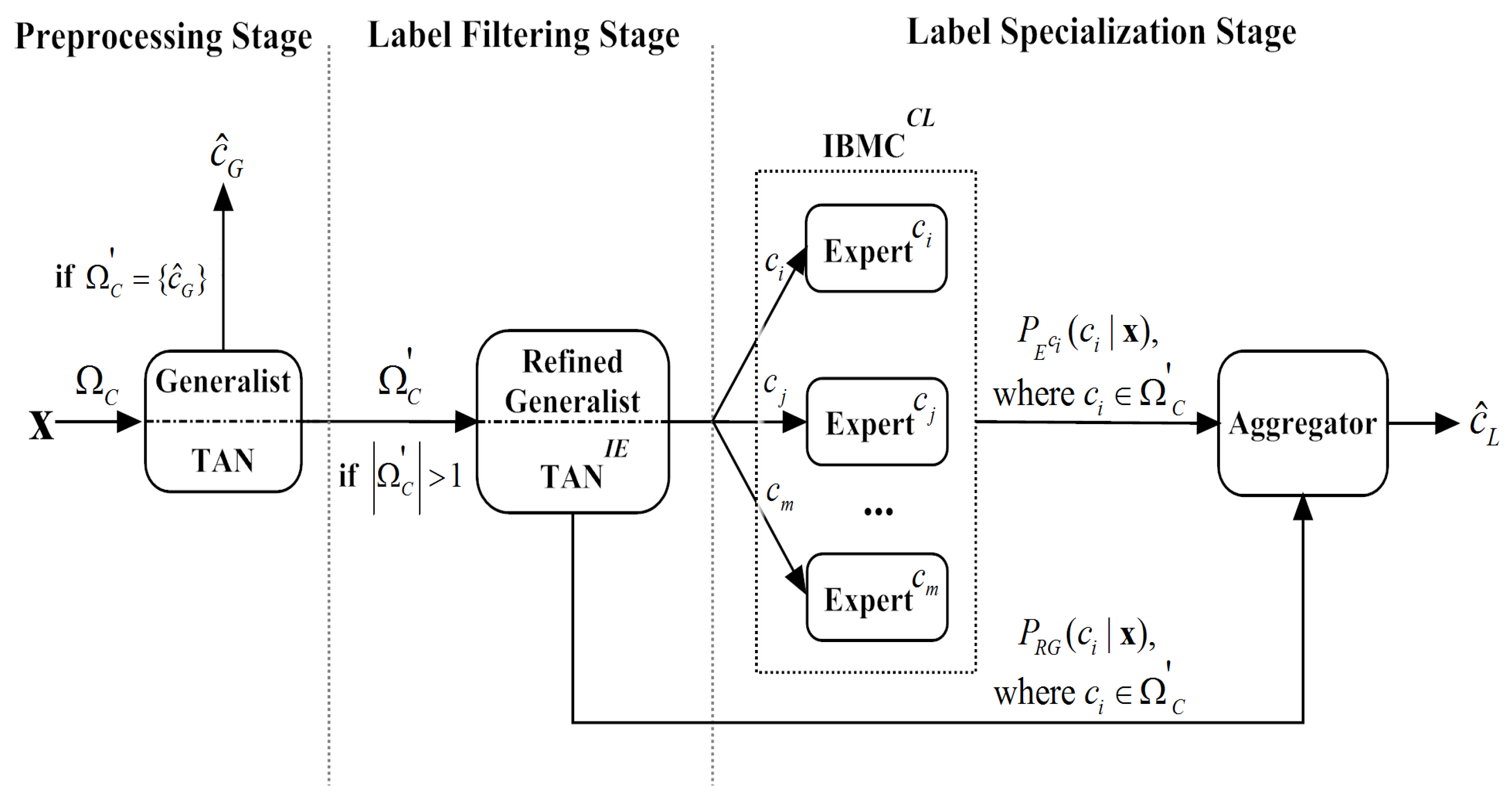
To provide a general view, we depict the architecture of the label-driven learning framework in Figure 3. We extend TAN to LTAN by applying the proposed framework. The framework leaves the training procedure of TAN (described in Algorithm 1) unchanged and only extends the classification procedure. The revised classification procedure is presented in Algorithm 4.
At training time, LTAN directly employs Algorithm 1 to train a TAN model, which has time complexity [2], where t is the number of training instances. At classification time, the label-driven learning framework is introduced. In the preprocessing stage, the time complexity of classifying a single testing instance with the generalist TAN is . Calculating to decide whether a testing instance needs to be reconsidered or not requires time . For testing instances whose includes only, will be returned as the predicted label and Algorithm 4 is terminated, resulting in the same classification time complexity as TAN . As for testing instances satisfying , the label filtering stage and the label specialization stage will be carried out. In the label filtering stage, firstly, the matrix is calculated, an operation of time complexity , where and v is the maximum number of values that an attribute may take. Then, the refined generalist TAN is built, which can be accomplished in . Finally, utilizing TAN to estimate posterior probabilities of labels in is of time complexity . In the label specialization stage, Algorithm 4 loops over each label in to learn IBMC. Inside the loop, computing the matrix and learning to be an expert of the given label both require time . Therefore, the overall time complexity of learning experts is . Estimating posterior probabilities with experts takes time . Finally, predictions of the refined generalist and experts are aggregated, with time complexity . From the above analysis, we can see that the time complexity of Algorithm 4 is dominated by the matrix calculation. Consequently, classifying a reconsidered testing instance with the label-driven learning framework has time complexity , while the time complexity of classifying a testing instance whose includes only is identical to that of TAN.
| Algorithm 4: The label-driven learning framework applied to TAN. |
 |
The label-driven learning framework takes time to classify a reconsidered testing instance, which is higher than of TAN. However, in practice, a large portion of testing instances will not be reconsidered (the detailed statistics are presented in Section 4.3). As a result, the framework will not incur too much computation overhead. Furthermore, we will show in Section 4.3.1 that given a proper , can be reduced to . Therefore, the label-driven learning framework embodies a good trade-off between computational efficiency and classification accuracy.
4. Empirical Study
We organize our extensive experiments from the following three aspects. To begin with, the threshold for label filtering of LTAN () is determined empirically in Section 4.1. Subsequently, to validate the effectiveness of the proposed label-driven learning framework, LTAN with the chosen threshold is compared with three single-structure BNCs: NB, TAN and KDB, as well as three ensemble BNCs: AODE, WATAN and AKDB in Section 4.2. Then, we analyze the performance of our novel label-driven learning framework in Section 4.3. Effects of the label filtering stage and the label specialization stage are investigated in Section 4.3.1 and Section 4.3.2, respectively. Training and classification time comparisons of TAN, LTAN and AKDB are provided in Section 4.4.
We run the above experiments on 40 benchmark datasets from the UCI machine learning repository [14]. Table 3 describes the detailed characteristics of these datasets in ascending order of their sizes, including the number of instances, attributes and classes. As listed in the table, the dataset size ranges from 32 instances of Lung Cancer to 5,749,132 instances of Donation, enabling us to examine classifiers on datasets with various sizes. Meanwhile, the number of class labels also spans from 2 to 50, allowing us to observe the performance of our label-driven learning framework on datasets with a wide range of label numbers. For each dataset, numeric attributes, if any, are discretized using Minimum Description Length Discretization (MDL) [27] as BNCs discussed in this paper cannot handle continuous attributes directly. Missing values are regarded as a distinct value. All of our experimental results are obtained via 10-fold cross-validation. Since some researchers report that the m-estimation leads to more accurate probabilities than the Laplace estimation [6,28,29], probability estimates are smoothed using the m-estimation (m = 1).
4.1. Selection of the Threshold for Label Filtering
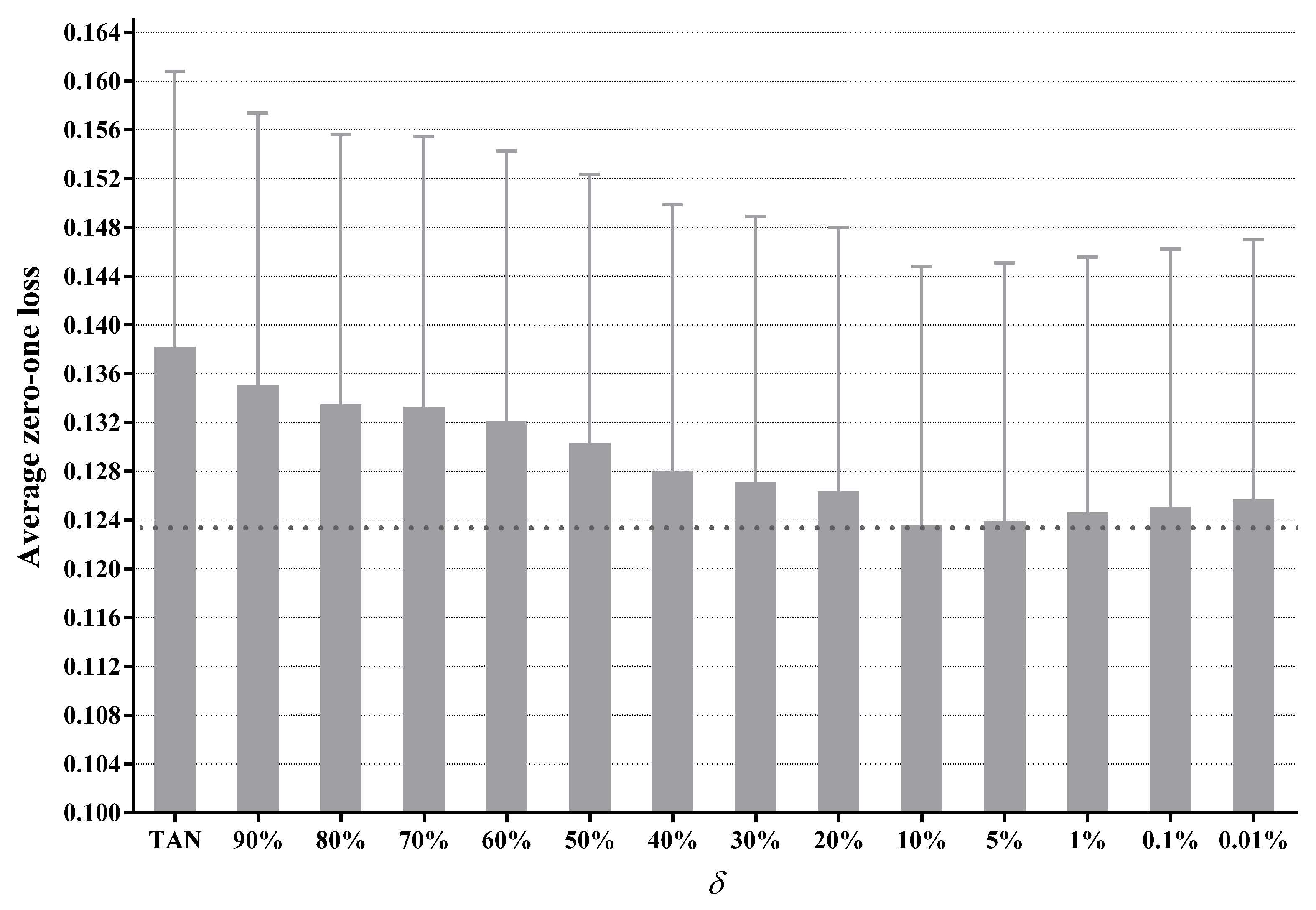
To apply our label-driven learning framework, we must first choose a threshold for label filtering, i.e., in Equation (14). As there does not appear to be any formal method to select an appropriate value for , we perform an empirical study to select it. Figure 4 presents the average zero-one loss results of LTAN across 40 datasets with different values. The standard error of each average zero-one loss is shown as well. To appreciate the effects of applying different , only the upper halves of the error lines are depicted. The experimental results of TAN are also shown in Figure 4 for comparison.
Figure 4 displays that, for all settings of , LTAN enjoys lower average zero-one loss compared to TAN. As decreases from 90% to 10%, the average zero-one loss declines steadily. This performance gain can be attributed to the fact that a smaller value can reduce the risk of leaving out the true label by retaining more labels, meanwhile enabling the label-driven learning framework to be applied to more testing instances. However, when is smaller than 10%, the average zero-one loss demonstrates a slight upward trend. One possible reason for this performance degradation is that, if is too small, many untrue class labels that carry low-confidence information will be retained, leading to unreasonable network structures.
It is empirically shown that LTAN achieves the lowest average zero-one loss when is set to 10%. Consequently, the setting is selected in our current work.
4.2. Comparisons in Terms of Zero-One Loss
In order to validate the effectiveness of the proposed label-driven learning framework, we conduct zero-one loss comparisons for related models that are divided into two groups: single-structure models and ensemble models. We compare LTAN with NB, TAN and KDB in the first group. Since at most one attribute parent is allowed for each attribute in LTAN, to make a fair comparison, we restrict KDB to a one-dependence classifier (). Technically speaking, LTAN is an ensemble of TAN and IBMC. Hence, this raises the issue that the advantage of LTAN over single-structure classifiers can be attributed to the superiority of its aggregation mechanism. To guard against this, we also compare LTAN with three ensemble classifiers in the second group: AODE, WATAN and AKDB ().
Table 4 reports for each dataset the average zero-one loss, which is assessed by 10-fold cross-validation. The symbols ∘ and • in Table 4, respectively, represent whether LTAN has zero-one loss improvement or degradation of at least 5% over TAN. In addition, the corresponding win/draw/loss records are summarized in Table 5. Cell in the table contains the number of wins/draws/losses for the classifier on row i against the classifier on column j. A win indicates that an algorithm reduces the zero-one loss of its opponent by at least 5%. A loss suggests the opposite situation. Otherwise, we consider that two classifiers perform equally well. Furthermore, standard binomial sign tests, assuming that wins and losses are equiprobable, are applied to these records. We assess a difference as significant if the outcome p of a one-tailed binomial sign test is less than 0.05. Significant win/draw/loss records are shown in bold in Table 5.
As shown in Table 4 and Table 5, in the single-structure classifier group, LTAN significantly outperforms NB and KDB. Most importantly, LTAN substantially improves upon the zero-one loss of TAN with 27 wins and only 4 losses, providing solid evidence for the effectiveness of the proposed label-driven learning framework. This advantage is even stronger for large datasets (20 datasets with more than 2000 instances). From Table 4, we can see that LTAN never loses on large datasets and exhibits significantly higher accuracy on 16 out of 20 large datasets.
When it comes to the ensemble group, LTAN still has a significant advantage over WATAN and AKDB. In addition, the comparison result with AODE is almost significant (). Although WATAN delivers significantly larger conditional log likelihood than TAN, when evaluated on zero-one loss, draws account for the majority of all comparisons (33 draws out of 40 datasets). Barely any zero-one loss advantage of WATAN over TAN is shown. Based on this fact, we argue that our LTAN is a more effective ensemble of TAN in terms of classification accuracy.
Demšar recommends the Friedman test [30] for comparisons of multiple algorithms over multiple data sets [31]. It ranks the algorithms for each data set separately: the best performing algorithm getting the rank of 1, the second best ranking 2, and so on. In case of ties, average ranks are assigned. The null-hypothesis is that all of the algorithms perform almost equivalently and there is no significant difference in terms of average ranks. The Friedman statistic can be computed as follows:
where and is the rank of the j-th of t algorithms on the i-th of N datasets. The Friedman statistic is distributed according to with degrees of freedom. Thus, for any pre-determined level of significance , the null hypothesis will be rejected if . The critical value of for with six degrees of freedom is 12.592. The Friedman statistic of experimental results in Table 4 is 57.806, which is larger than 12.592. Hence, the null-hypotheses is rejected.
Since the null-hypotheses is rejected, the Nemenyi test [32] is used to further analyze which pairs of algorithms are significantly different in terms of average ranks of the Friedman test. The performance of two classifiers is significantly different if their corresponding average ranks of the Friedman test differ by at least the critical difference ():
where the critical value for and is 2.949 [31]. Given seven algorithms and 40 datasets, can be calculated with Equation (20) and is equal to 1.4245. Following the graphical presentation proposed by Demšar [31], we show the comparison of these algorithms against each other with the Nemenyi test in Figure 5. We plot the algorithms on the bottom line according to their average ranks, which are indicated on the parallel upper axis. The axis is turned so that the lowest (best) ranks are to the right since we perceive the methods on the right side as better. The algorithms are connected by a line if their differences are not significant. is also presented in the graph. As shown in Figure 5, the average rank of LTAN is significantly better than that of TAN, proving the effectiveness of the proposed label-driven learning framework. Although LTAN ranks first, its advantage is not significant compared to AKDB or AODE.
4.3. Analysis of the Label-Driven Learning Framework
As specified in Section 3.4, the time complexity of classifying a reconsidered testing instance with the label-driven learning framework is , which is higher than of TAN. If a large portion of testing instances are reconsidered, on one hand the label-driven learning framework can exert a strong influence on the classification task; on the other hand, considerable computation overhead will be incurred. This is essentially a trade-off between computational efficiency and classification accuracy. The set of testing instances satisfying the reconsideration condition in testing cases of a dataset can be denoted as:
where x is a testing instance, is the testing set and can be obtained using Equation (14). Thus, label-driven learning percentage () can be defined as follows:
Definition 9.
The label-driven learning percentage () for a dataset is the proportion of reconsidered testing instances in the testing set. It can be calculated by
where R is the reconsidered testing instance set obtained using Equation (21), and is the testing set.
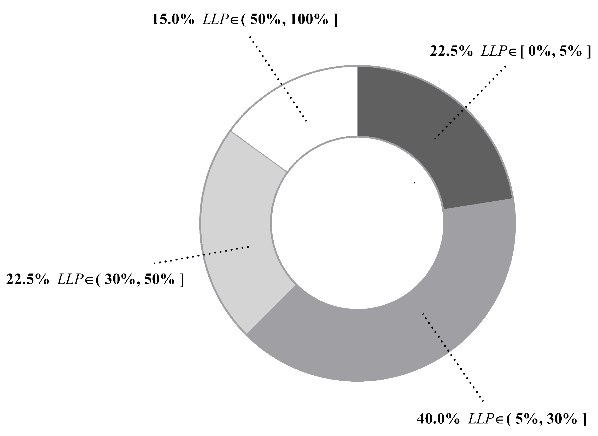
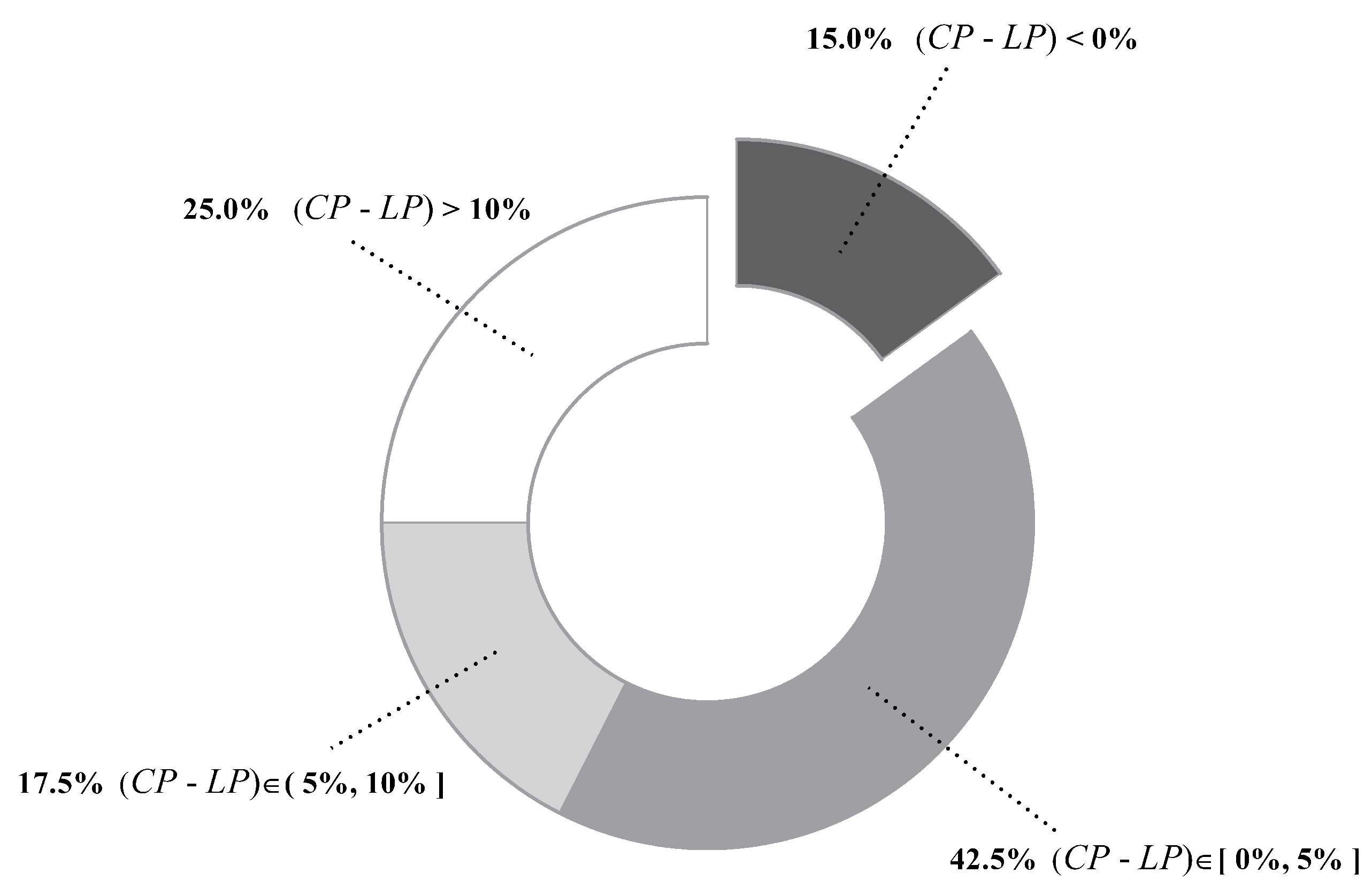
Figure 6 presents values of all datasets. We can see that differs greatly from dataset to dataset, ranging from 0.01% of Mushrooms (No. 29) to 99.86% of Poker-hand (No. 39). To give an intuitive illustration, percentages of datasets whose values fall in different ranges are depicted in Figure 7. The chart shows that, for 85% of datasets, less than half of testing instances are reconsidered and, for 62.5% of datasets, less than 30% of testing instances are reconsidered. These facts suggest that, in many datasets, a large portion of testing instances just simply employ a TAN classifier. Therefore, the label-driven learning framework will not incur too much computation overhead. Although the framework is applied to less than 30% of testing instances on 62.5% of datasets, it still manages to improve the classification accuracy of TAN significantly on 17 out of 25 such datasets. The values on six datasets are greater than 50%. An extreme example is Poker-hand, whose is surprisingly high (99.86%). Almost all of the testing instances in Poker-hand are reconsidered, dramatically reducing the classification error of TAN by 31.23% at the cost of computational efficiency.
The above LLP analysis shows that our label-driven learning framework can offer a trade-off between computational efficiency and classification accuracy. However, the LLP analysis is not sufficient. As specified above, BNCs tend to misclassify testing instances where some labels bear high confidence degrees close to that of the predicted label. Such instances are included in R, which is defined in Equation (21). Our framework is intended to alleviate this problem. To determine whether it is successful at this goal, we propose two new criteria: correction percentage () and loss percentage (). They can evaluate the ability of the framework to correct misclassifications of the generalist and meanwhile avoid causing offsetting errors in R. and are defined as follows:
Definition 10.
The correction percentage () for a dataset measures the proportion of instances in R, which are misclassified by the generalist, but correctly classified by the label-driven learning framework. It can be calculated by
where is the true class label ofx, and is the label predicted by TAN and LTAN, respectively.
Definition 11.
The loss percentage () for a dataset measures the proportion of instances in R, which are correctly classified by the generalist, but misclassified by the label-driven learning framework. It can be calculated by
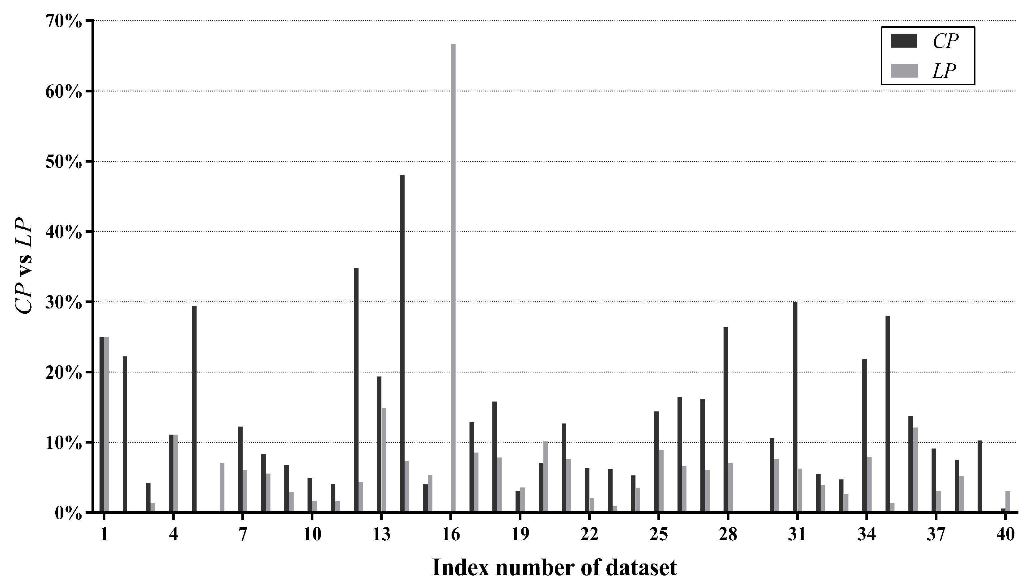
Figure 8 compares with on each dataset. In addition, percentages of datasets whose values fall in different ranges are summarized in Figure 9. For the majority of datasets (85%), is higher than , suggesting that our label-driven learning framework can correct incorrect predictions of TAN more often than making new mistakes in R. Most notably, is evidently higher than for over 10% in 10 datasets. In all 10 of these datasets, LTAN obtains significantly lower error than TAN. A notable case is Cylinder-bands (No. 14), where the learning framework reduces the classification error of TAN by 39.85% with a difference of 40.67% between and . For 17.5% of datasets, although the difference between and is less obvious (5% to 10%), similar results that LTAN wins on all these datasets in terms of zero-one loss are still observed. For 42.5% of datasets, is slightly higher than , resulting in 10 wins out of 17 datasets with respect to zero-one loss. However, there are 15% of datasets whose is lower than . TAN is affected negatively by the learning framework on these datasets. A typical example is Syncon (No. 16). Disappointingly, its reaches 66.67% with a 0% value. However, we must notice that the value of Syncon is only 0.5%, indicating that merely 3 out of its 600 instances are reconsidered. Among these three instances, two instances are misclassified by LTAN although TAN can correctly classify them. Considering the outstanding performance of our learning framework on other datasets, failures for two instances of Syncon are tolerable.
The above results prove that our framework can alleviate the misclassification problem of the generalist TAN and meanwhile make a few new mistakes on testing instances in R, leading to the substantially higher classification accuracy of LTAN over TAN.
4.3.1. Effects of the Label Filtering Stage
In the label filtering stage, our framework removes labels that are highly unlikely to be the true label, reducing the label space from to . As specified in Section 3.4, for reconsidered testing instances, the time complexity of LTAN at classification time is , where n is the number of attributes, v is the maximum number of values that an attribute may take and . With n and v in both determined by a dataset, the number of remaining labels, r, plays a vital role in the classification time complexity. In this subsection, we will discuss r in detail.
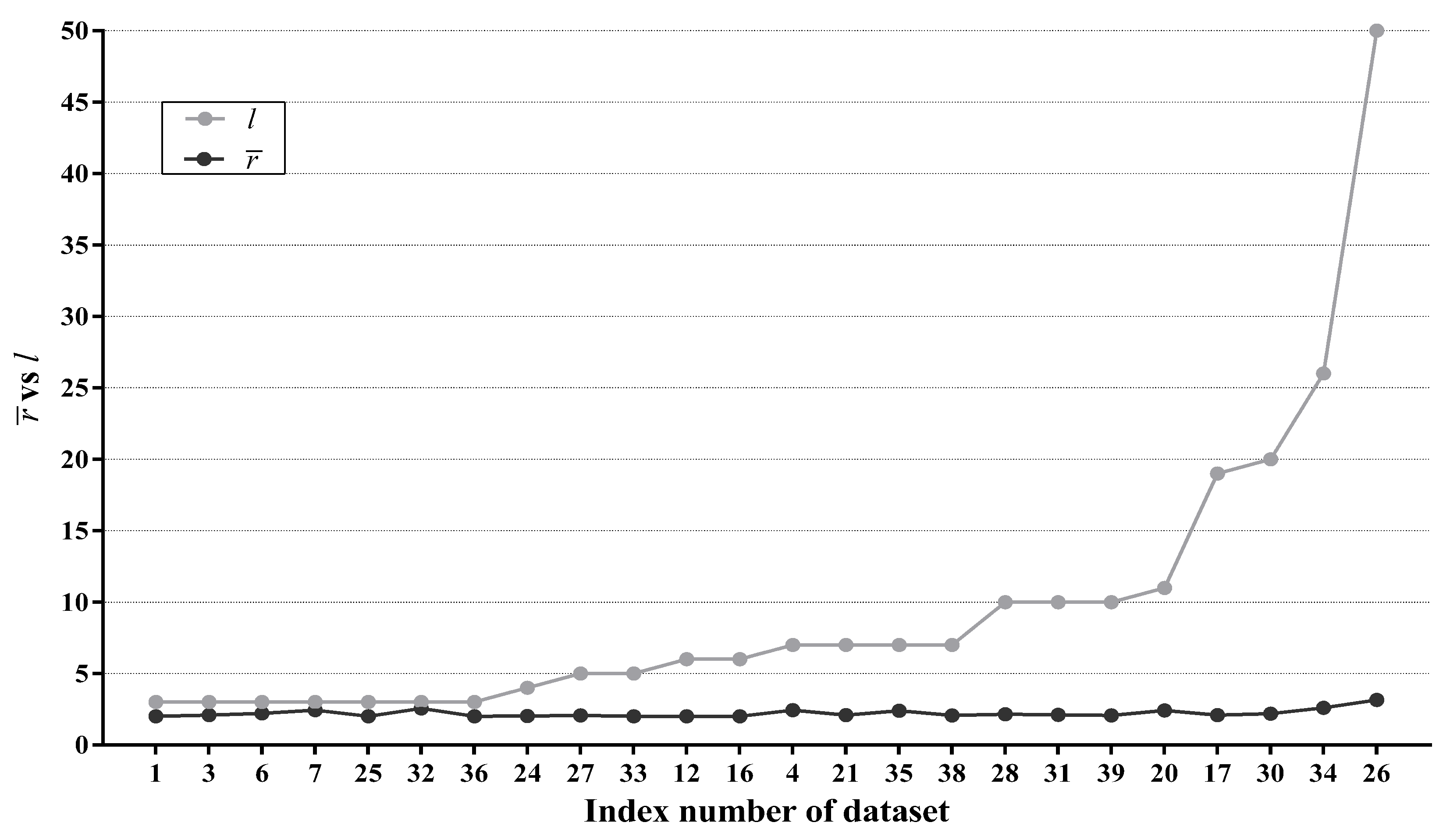
It is worth mentioning that, for binary classification problems, LTAN either degrades to TAN when , or removes no labels at all in the opposite situation. Thus, for a binary classification problem, r is always equal to 2. For each multi-class dataset, we compute the average r value of reconsidered testing instances, denoted as . Figure 10 presents the result along with the original number of class labels l for each multi-class dataset. Note that the 24 multi-class datasets in Figure 10 are ordered according to l.
As shown in Figure 10, the growth rate of is not in proportion to the growth rate of l. Instead, fluctuates slightly between two and three regardless of how many labels a dataset originally has, indicating that, on average, only two or three labels require further discrimination. Especially for Phoneme (No. 26), only 3 out of 50 class labels survive the label filtering. Consequently, we can consider r as a constant, reducing the classification time complexity of LTAN for reconsidered testing instances from to . Although is still higher than of TAN, considering the superiority of LTAN over TAN from the viewpoint of classification accuracy, this computation overhead is reasonable.
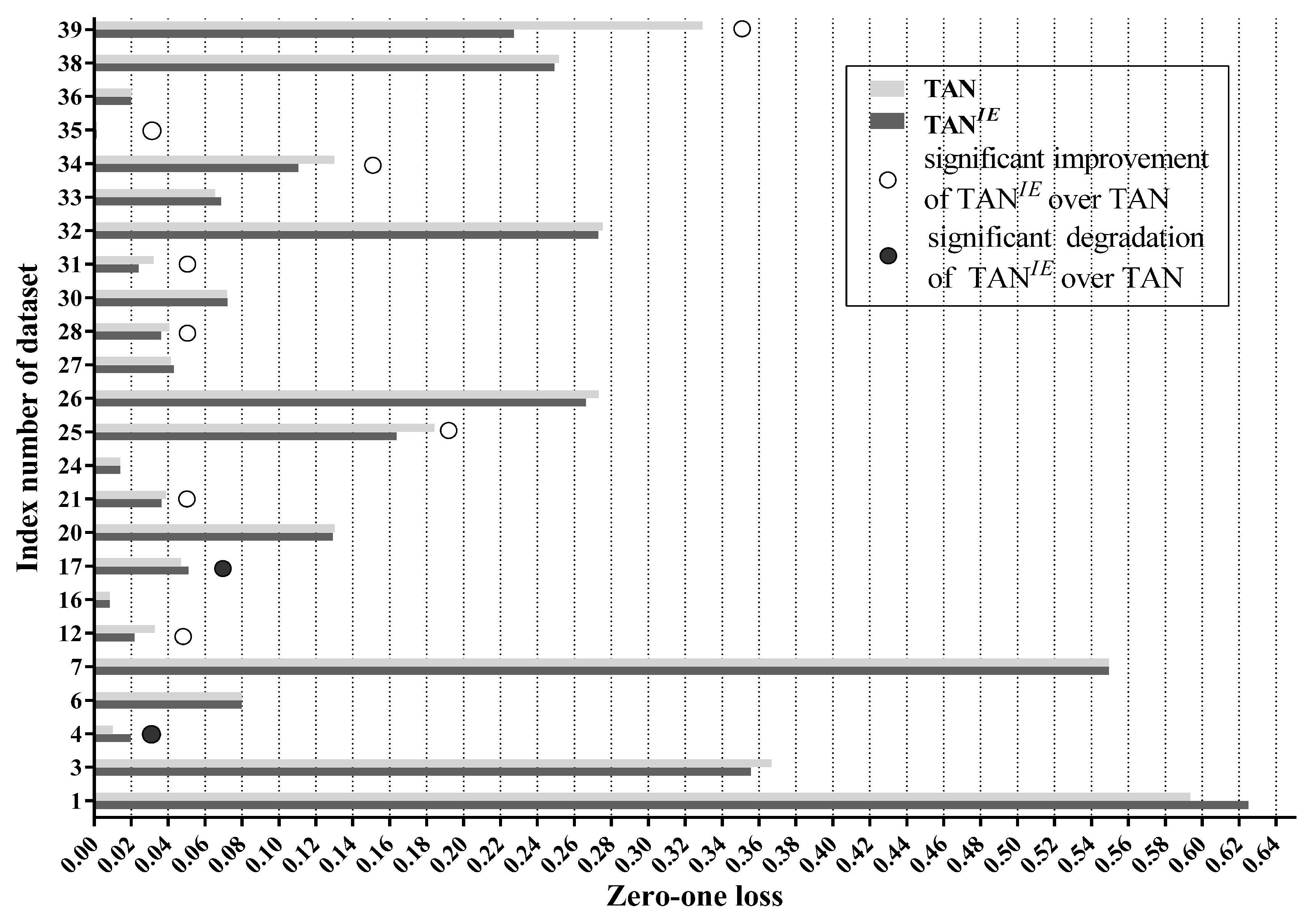
After filtering out low-confidence labels, TAN reconstructs the MST of TAN with information derived from remaining labels. For binary classification problems, no class labels of instances in R are deleted at all. As a result, TAN has exactly the same structure as TAN, leading to the same classification accuracy as TAN. We can thus conclude that the label filtering stage has no effect for binary classification problems. This, however, does not mean that our label-driven learning framework is invalid for binary classification problems. On the contrary, thanks to IBMC, LTAN achieves substantially lower error than TAN on 10 out of 16 binary-label datasets. To reveal whether the label filtering stage can really increase the classification accuracy of TAN on multi-class datasets, we compare the zero-one loss of TAN with that of TAN in Figure 11 in these datasets.
Figure 11 shows that the label filtering stage significantly improves the classification accuracy of TAN on 8 out of 24 multi-class datasets. A notable case is Poker-hand (No. 39) where the label filtering stage achieves a 31.02% zero-one loss improvement. In addition, the performance degradation of TAN over TAN is significant only in two datasets. The inferiority of TAN on Zoo (No. 4) and Soybean (No. 17) may result from lacking enough training data. TAN are trained using instances belonging to remaining labels only. The average number of remaining labels of reconsidered testing instances, namely , on Zoo is 2.4444. Zoo has 101 instances and 7 class labels. Hence, TAN of Zoo only has approximately 31.74 instances for training on average. Similarly, TAN of Soybean has 67.48 instances for training on average. Accurate estimations of edge weights of TAN, i.e., in Equation (16), is determined by precise probability estimation, which is hard to ensure with limited training data. Therefore, the reconstruction of MST is affected negatively by inaccurate estimations of on Zoo and Soybean, leading to unreasonable network structures. With 8 wins and 2 losses, we can infer that the label filtering stage can help reduce the classification error of TAN to some extent. For the rest of 24 datasets (14 datasets), the performance of TAN compared to TAN is similar, indicating that the label filtering stage has few effects on these datasets. The reason may be that some attributes are strongly related to each other. Eliminating information derived from low-confidence labels can not affect their dependence. Consequently, same dependence relations between these attributes may appear in both TAN and TAN. On datasets with such attributes, TAN and TAN may have similar structures and thus show equivalent performance.
4.3.2. Effects of the Label Specialization Stage
The label filtering stage has no effect on binary classification problems. To address this deficiency and further discriminate among high-confidence labels, our framework has an extra stage compared with the two-stage learning paradigm proposed in [13], namely the label specialization stage, wherein a set of experts is built. Then, LTAN, an ensemble of the refined generalist TAN and the expert set IBMC, is returned as the final classifier. To justify the addition of the label specialization stage, we investigate whether the experts can work as an effective complementary part of the refined generalist. For this purpose, the diversity between them can be an appropriate indicator. Diversity has long been recognized as a necessary condition for improving ensemble performance, since, if base classifiers are highly correlated, it is not possible to gain much by combining them [33]. Hence, the key to successful ensemble methods is to construct individual classifiers whose predictions are uncorrelated.
Since WATAN is also a TAN ensemble classifier, we can compare the diversity between TAN and IBMC with the diversity of the subclassifiers of WATAN. In order to measure diversity, we adopt the statistic [34], which is defined as follows:
Definition 12.
Given a pair of classifiers, and , the κ statistic measures their degree of agreement. Suppose there are l class labels, and let D be a square array such that contains the number of testing instances assigned to class label i by and into class label j by . Thus, the κ statistic can be calculated as:
where is the probability that the two classifiers agree, and is the probability that the two classifiers agree by chance; they are respectively defined as:
where m is the total number of testing instances. when the agreement of the two classifiers equals that expected by chance, and when the two classifiers agree on every example. Negative values occur when their agreement is weaker than expected by chance.
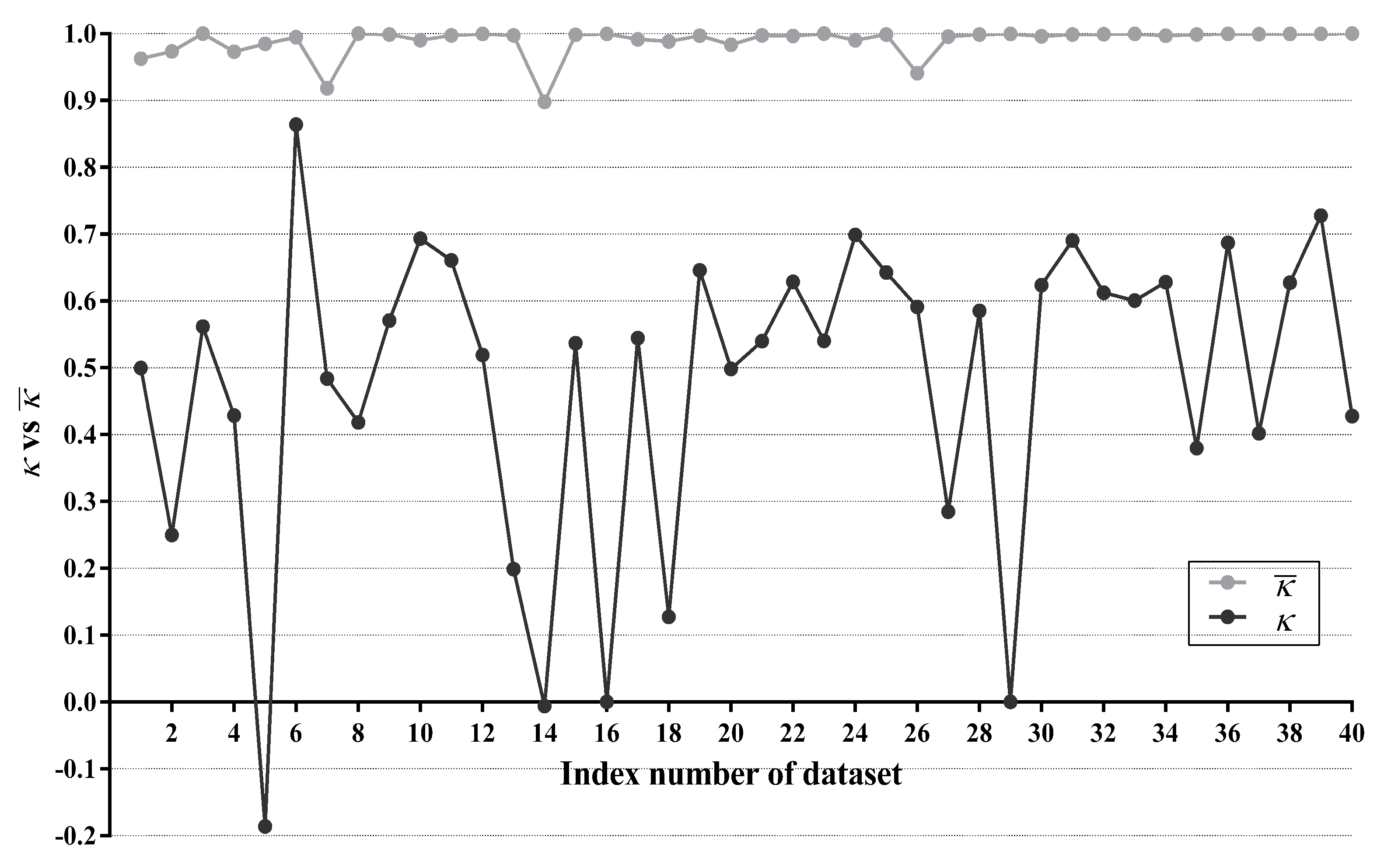
For WATAN, the average of statistics between every two subclassifiers is computed, denoted as . For LTAN, we calculate the statistic between TAN and IBMC using only testing instances in R, denoted as . Figure 12 compares with on each dataset.
As shown in Figure 12, values on 31 datasets (40 datasets in total) are higher than 0.99, which is very close to 1. The lowest is achieved on Cylinder-bands (No. 14). However, it is still as high as 0.898. It is evident that the subclassifiers of WATAN often reach very high agreement and demonstrate poor diversity. There is little chance for a subclassifier of WATAN to revise wrong predictions made by its counterparts. Owing to this reason, the zero-one loss improvement of WATAN over TAN is only marginal (5 wins out of 40 datasets). Obviously, TAN and IBMC have substantially larger diversity than the subclassifers of WATAN.On dataset Cylinder-bands (No. 14), Syncon (No. 16) and Mushrooms (No. 29), statistics are very close to 0, indicating that TAN and IBMC agree only by chance on these datasets. The statistic is negative (−0.186) on Promoters (No. 5). This suggests that TAN tends to disagree with IBMC on Promoters. By making different predictions, some misclassifications of TAN may be corrected by IBMC. As a matter of fact, experimental results in Section 4.3.1 show that TAN only wins on 8 out of 24 multi-class datasets compared with TAN. Moreover, TAN has the same network structures and same classification accuracy with TAN on 16 binary-label datasets. With the help of IBMC, LTAN, the ensemble of TAN and IBMC, wins on 17 out of 24 multi-class datasets and 10 out of 16 binary-label datasets. We can thus conclude that the classification accuracy of TAN can be significantly enhanced by the addition of IBMC.
The refined generalist TAN and the expert set IBMC often make different predictions and demonstrate large diversity. By making different predictions, misclassifications of the refined generalist may be corrected by the experts. Therefore, the experts can serve as an effective complementary part of the refined generalist. Jointly applying both the label filtering stage and the label specialization stage can achieve a significant improvement over TAN in terms of classification accuracy.
4.4. Time Comparisons of TAN, LTAN and AKDB
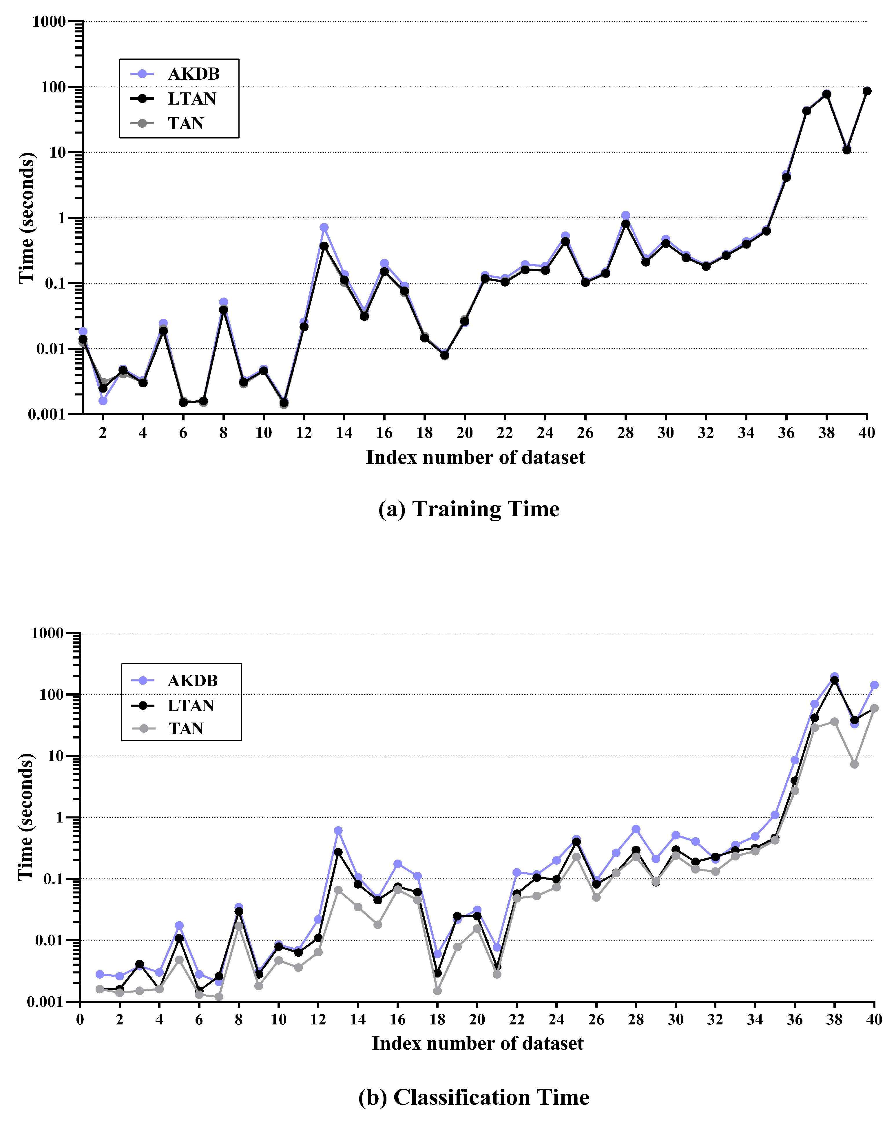
The label-driven learning framework leaves the training procedure of TAN unchanged and only extends the classification procedure. Classifying a reconsidered testing instance with the framework is of time complexity , which is higher than of TAN. For those testing instances which do not require reconsideration, the classification time complexity is identical to that of TAN. As introduced in Section 2.2.3, similar to LTAN, AKDB also adopts instance-based learning. AKDB with shares the same training time complexity as TAN. At classification time, AKDB with learns a one-dependence LKDB for each testing instance, a procedure with time complexity , which is usually a bit lower than . Figure 13 presents training time and classification time comparisons of TAN, LTAN and AKDB per dataset. These experiments have been conducted on a desktop computer with an Intel(R) Core(TM) i3-2310M CPU @ 2.10 GHz, 2.10 GHz, 64 bits and 8G of memory. No parallelization techniques have been used in any case. The reported training or classification time is averaged over five runs of 10-fold cross validation. It is important to note that logarithmic scale is used in Figure 13.
As shown in Figure 13a, LTAN requires almost the same training time as TAN. AKDB takes a bit more training time, due to its attribute ranking and parent assignment procedure. Although the time complexity of classifying a reconsidered testing instance and classifying a testing instance using AKDB are both quadratic with respect to the number of attributes n, as shown in Figure 13b, LTAN often enjoys advantages over AKDB in terms of classification time while suffering classification time disadvantages over TAN. The reason lies in that a large portion of testing instances on many datasets are not reconsidered, in other words, values (defined in Equation (22)) on many datasets are low. A typical example is Musk1 (No. 13), which has 166 attributes. On Musk1, AKDB requires substantially more classification time than TAN, 0.6139 s compared to 0.0658 s of TAN. As 14.08% of testing instances are reconsidered on Musk1, LTAN spends 0.2729 s, which is twice as fast as AKDB. Another outstanding example is Shuttle (No. 35). LTAN achieves a significant zero-one loss improvement on Shuttle by reconsidering only 0.25% of testing instances, which merely takes extra 0.0380 s. AKDB, however, spends 0.6808 more seconds than TAN. However, when is large, the computation overhead of applying the label-driven learning framework will be high. For example, almost all testing instances of Poker-hand (No. 39) are reconsidered. Hence, the classification time of TAN increases sharply from 7.2917 s to 38.5678 s, whereas AKDB spends 32.8171 s. On Covtype (No. 38) with 58.95% LLP and 54 attributes, it takes LTAN 170.1345 s and AKDB 196.6520 s to finish the classification procedure, while TAN only takes 36.1403 s. Fortunately, as specified in Section 4.3, for 85% of datasets, less than half of testing instances are reconsidered and for 62.5% of datasets, less than 30% of testing instances are reconsidered. Consequently, the negative effect of using an algorithm with classification time complexity quadratic in n can be greatly mitigated.
To conclude, compared to AKDB, LTAN not only has higher classification accuracy (although not statistically significant using the Nemenyi test), but also generally lower classification time. Compared to TAN, LTAN delivers significantly lower zero-one loss, without incurring too much computation overhead on average.
5. Discussion
On datasets from Table 6, the classification accuracy of LTAN degrades significantly compared to TAN. On these datasets, the label-driven learning framework makes new mistakes more often than correcting incorrect predictions of TAN, i.e., ( and are defined in Equations (23) and (24), respectively), and thus has negative effects . We believe that expert classifiers are responsible for this problem. Theoretically, experts can provide more accurate posterior probability estimations. However, in practice, their network structures are sometimes unreasonable due to lack of enough training data and hence their performance of probability calibration is poor.
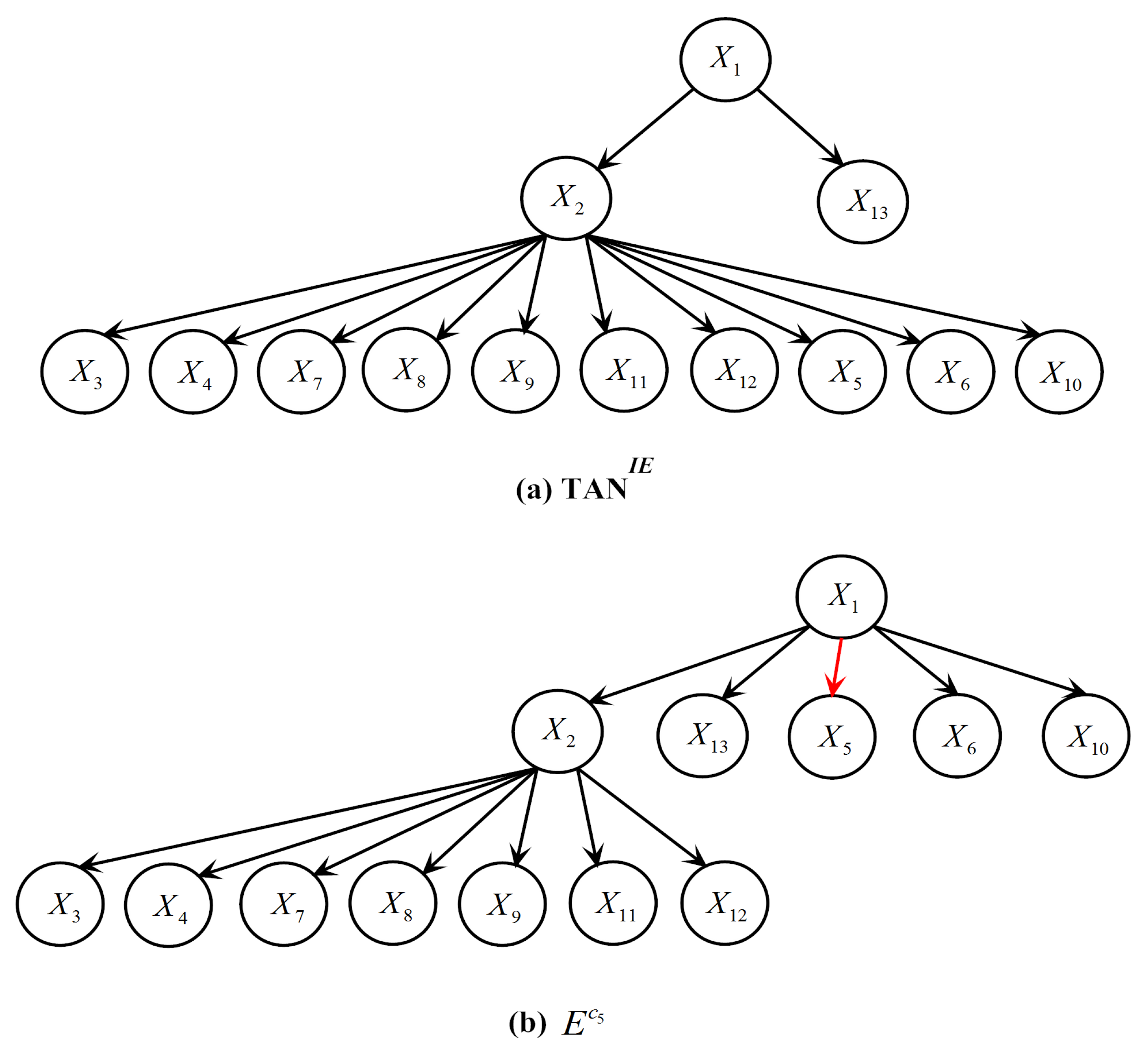
For ease of analysis, Table 7 presents a typical testing instance in Vowel that is misclassified by LTAN but correctly classified by TAN. Additionally, its class membership probabilities estimated by TAN, TAN, IBMC and LTAN are shown in Table 8. Similar testing instances with the same problem can be found in other datasets in Table 6. The true label of the testing instance in Table 7 is . The refined generalist TAN predicts a reasonable posterior probability for (0.8215). However, the probability produced by the expert E is surprisingly low (0.0185), making the average posterior probability for 0.42, which is smaller than that of . To investigate the reason for the incorrect probability estimation, the network structures of TAN and E for the testing instance are shown in Figure 14. Note that the class label is not depicted in Figure 14 for simplicity.
Figure 14 shows that the attributes (except , and ) have the same parents in the refined generalist and E, leading to the same probability terms. In addition, the differences between and or and are not large, where and denote the probabilities estimated by the refined generalist and the expert of respectively. However, is equal to 0.1267, whereas only has a value of 0.0028 because , where denotes the frequency of a combination appears in the training set. Consequently, having as the parent of causes the posterior probability of to drop sharply. The arc connecting and is highlighted in red in Figure 14. As a matter of fact, the between and is much greater than and any other attributes. Although Vowel has 990 testing instances, it has 11 labels and thus each expert has only 84 instances for training (Vowel is a balanced dataset). In the training set of E, only appears five times, resulting in a negative between and (the between and is 0). E severely underestimates the dependence between and . If given enough training data, E can detect their dependence relationship and provides an accurate posterior probability estimation for .
Similar to Vowel, experts on the Iris, Chess and Syncon datasets all suffer from the insufficient training data problem. Learning an expert per class instead of one overall structure requires enough training instances. When the dataset size is larger than 2000 instances, the label-driven learning framework corrects possible misclassifications of reconsidered testing instances without making too many offsetting errors.
6. Conclusions
To further discriminate among high-confidence labels, we develop the label-driven learning framework, which is composed of three components: the generalist, the refined generalist and the experts. They form a three-level hierarchy, with increasing degree of localisation. By providing solid empirical comparisons with several state-of-the-art single-structure BNCs (NB, TAN and KDB), as well as three established ensemble BNCs (AODE, WATAN and AKDB), we prove that this framework can help correct possible misclassifications of TAN without causing too many offsetting errors or incurring very high computation overhead.
There are two immediate directions for future work. Firstly, the label-driven learning framework can be homogeneous or heterogeneous. Immediate future work for homogeneous label-driven learning frameworks is to apply the framework to other BNCs like KDB. Heterogeneous label-driven learning frameworks that are more flexible fall outside the scope of this paper and will be studied in our future work. Furthermore, in our current work, the threshold for label filtering, i.e., in Equation (14), is pre-determined using an empirical study. To optimize the parameter on a particular dataset, we can randomly select a portion of the training data as a holdout set. After training the generalist using the remaining training data, the performance of all candidates will be tested on the holdout set and the one with the highest classification accuracy will be selected.
Acknowledgments
This work was supported by the National Science Foundation of China (Grant No. 61272209) and the Agreement of Science and Technology Development Project, Jilin Province (No. 20150101014JC).
Author Contributions
All authors have contributed to the study and preparation of the article. Yi Sun conceived the idea, derived equations and wrote the paper. Limin Wang and Minghui Sun did the analysis and finished the programming work. All authors have read and approved the final manuscript.
Conflicts of Interest
The authors declare no conflicts of interest.
References
- Bielza, C.; Larrañaga, P. Discrete bayesian network classifiers: A survey. ACM Comput. Surv. 2014, 47. [Google Scholar] [CrossRef]
- Friedman, N.; Geiger, D.; Goldszmidt, M. Bayesian network classifiers. Mach. Learn. 1997, 29, 131–163. [Google Scholar] [CrossRef]
- Sahami, M. Learning Limited Dependence Bayesian Classifiers. In Proceedings of the Second International Conference on Knowledge Discovery and Data Mining, Portland, Oregon, USA, 2–4 August 1996; pp. 335–338. [Google Scholar]
- Song, H.; Xu, Q.; Yang, H.; Fang, J. Interpreting out-of-control signals using instance-based Bayesian classifier in multivariate statistical process control. Commun. Stat. Simul. Comput. 2017, 46, 53–77. [Google Scholar] [CrossRef]
- Wang, L.; Zhao, H.; Sun, M.; Ning, Y. General and local: Averaged k-dependence bayesian classifiers. Entropy 2015, 17, 4134–4154. [Google Scholar] [CrossRef]
- Zheng, F.; Webb, G.I.; Suraweera, P.; Zhu, L. Subsumption resolution: An efficient and effective technique for semi-naive Bayesian learning. Mach. Learn. 2012, 87, 93–125. [Google Scholar] [CrossRef]
- Webb, G.I.; Boughton, J.R.; Wang, Z. Not so naive Bayes: Aggregating one-dependence estimators. Mach. Learn. 2005, 58, 5–24. [Google Scholar] [CrossRef]
- Jiang, L.; Cai, Z.; Wang, D.; Zhang, H. Improving tree augmented naive bayes for class probability estimation. Knowl. Based Syst. 2012, 26, 239–245. [Google Scholar] [CrossRef]
- Libal, U.; Hasiewicz, Z. Risk upper bound for a NM-type multiresolution classification scheme of random signals by Daubechies wavelets. Eng. Appl. Artif. Intell. 2017, 62, 109–123. [Google Scholar] [CrossRef]
- Das, N.; Sarkar, R.; Basu, S.; Saha, P.K.; Kundu, M.; Nasipuri, M. Handwritten bangla character recognition using a soft computing paradigm embedded in two pass approach. Pattern Recogn. 2015, 48, 2054–2071. [Google Scholar] [CrossRef]
- Liu, K.-H.; Yan, S.; Kuo, C.-C.J. Age estimation via grouping and decision fusion. IEEE Trans. Inf. Forensics Secur. 2015, 10, 2408–2423. [Google Scholar] [CrossRef]
- Grossi, G.; Lanzarotti, R.; Lin, J. Robust face recognition providing the identity and its reliability degree combining sparse representation and multiple features. Int. J. Pattern Recogn. 2016, 30, 1656007. [Google Scholar] [CrossRef]
- Godbole, S.; Sarawagi, S.; Chakrabarti, S. Scaling multi-class support vector machines using inter-class confusion. In Proceedings of the Eighth ACM SIGKDD International Conference on Knowledge Discovery and Data Mining, Edmonton, AB, Canada, 23–25 July 2002; pp. 513–518. [Google Scholar]
- Bache, K.; Lichman, M. UCI Machine Learning Repository. Available online: https://archive.ics.uci.edu/ml/datasets.html (accessed on 1 December 2017).
- Shannon, C. A mathematical theory of communications, I and II. Bell Syst. Tech. J. 1948, 27, 379–423. [Google Scholar] [CrossRef]
- Chen, S.; Martínez, A.M.; Webb, G.I.; Wang, L. Selective AnDE for large data learning: A low-bias memory constrained approach. Knowl. Inf. Syst. 2017, 50, 475–503. [Google Scholar] [CrossRef]
- Peng, H.; Fan, Y. Feature selection by optimizing a lower bound of conditional mutual information. Inf. Sci. 2017, 418, 652–667. [Google Scholar] [CrossRef]
- Cover, T.M.; Thomas, J.A. Elements of Information Theory, 2nd ed.; Wiley: Hoboken, NJ, USA, 2012; pp. 1–22. [Google Scholar]
- Liu, H.; Zhou, S.; Lam, W.; Guan, J. A new hybrid method for learning Bayesian networks: Separation and reunion. Knowle. Based Syst. 2017, 121, 185–197. [Google Scholar] [CrossRef]
- Bartlett, M.; Cussens, J. Integer linear programming for the Bayesian network structure learning problem. Artif. Intell. 2017, 244, 258–271. [Google Scholar] [CrossRef]
- Prim, R.C. Shortest connection networks and some generalizations. Bell Syst. Tech. J. 1957, 36, 1389–1401. [Google Scholar] [CrossRef]
- Martínez, A.M.; Webb, G.I.; Chen, S.; Zaidi, N.A. Scalable learning of bayesian network classifiers. J. Mach. Learn. Res. 2016, 17, 1515–1549. [Google Scholar]
- Pensar, J.; Nyman, H.; Lintusaari, J.; Corander, J. The role of local partial independence in learning of Bayesian networks. Int. J. Approx. Reason. 2016, 69, 91–105. [Google Scholar] [CrossRef]
- Dan, G.; Heckerman, D. Knowledge representation and inference in similarity networks and Bayesian multinets. Artif. Intell. 1996, 82, 45–74. [Google Scholar]
- Huang, K.; King, I.; Lyu, M.R. Discriminative training of Bayesian chow-liu multinet classifiers. In Proceedings of the International Joint Conference on Artificial intelligence, Acapulco, Mexico, 19–25 August 2003; pp. 484–488. [Google Scholar]
- Chow, C.; Liu, C. Approximating discrete probability distributions with dependence trees. IEEE Trans. Inf. Theory 1968, 14, 462–467. [Google Scholar] [CrossRef]
- Fayyad, U.M.; Irani, K.B. Multi-interval Discretization of Continuous-Valued Attributes for Classification Learning. In Proceedings of the 13th International Joint Conference on Artificial Intelligence, Chambery, France, 28 August–3 September 1993; pp. 1022–1029. [Google Scholar]
- Zaidi, N.A.; Cerquides, J.; Carman, M.J.; Webb, G.I. Alleviating naive bayes attribute independence assumption by attribute weighting. J. Mach. Learn. Res. 2013, 14, 1947–1988. [Google Scholar]
- Cestnik, B. Estimating probabilities: a crucial task in machine learning. In Proceedings of the Ninth European Conference on Artificial Intelligence, Stockholm, Sweden, 6–10 August 1990; pp. 147–149. [Google Scholar]
- Friedman, M. The use of ranks to avoid the assumption of normality implicit in the analysis of variance. J. Am. Stat. Assoc. 1937, 32, 675–701. [Google Scholar] [CrossRef]
- Demřar, J. Statistical comparisons of classifiers over multiple data sets. J. Mach. Learn. Res. 2006, 7. Available online: http://dl.acm.org/citation.cfm?id=1248547.1248548 (accessed on 1 December 2017).
- Nemenyi, P. Distribution-Free Multiple Comparisons. Ph.D. Thesis, Princeton University, Princeton, NJ, USA, 1963. [Google Scholar]
- Özöğür-Akyüz, S.; Windeatt, T.; Smith, R. Pruning of error correcting output codes by optimization of accuracy-diversity trade off. Mach. Learn. 2015, 101, 253–269. [Google Scholar] [CrossRef] [Green Version]
- Díez-Pastor, J.-F.; García-Osorio, C.; Rodríguez, J.J. Tree ensemble construction using a grasp-based heuristic and annealed randomness. Inf. Fusion. 2014, 20, 189–202. [Google Scholar] [CrossRef]
Figure 1.
Examples of network structures with four attributes for the following BN classifiers: (a) NB; (b) TAN; (c) KDB (k = 2).
Figure 1.
Examples of network structures with four attributes for the following BN classifiers: (a) NB; (b) TAN; (c) KDB (k = 2).

Figure 2.
An example of a BMC with two local BNs.

Figure 3.
Architecture of the label-driven learning framework.

Figure 4.
The average zero-one loss of LTAN across 40 datasets with different values.

Figure 5.
Zero-one loss comparison with the Nemenyi test. .
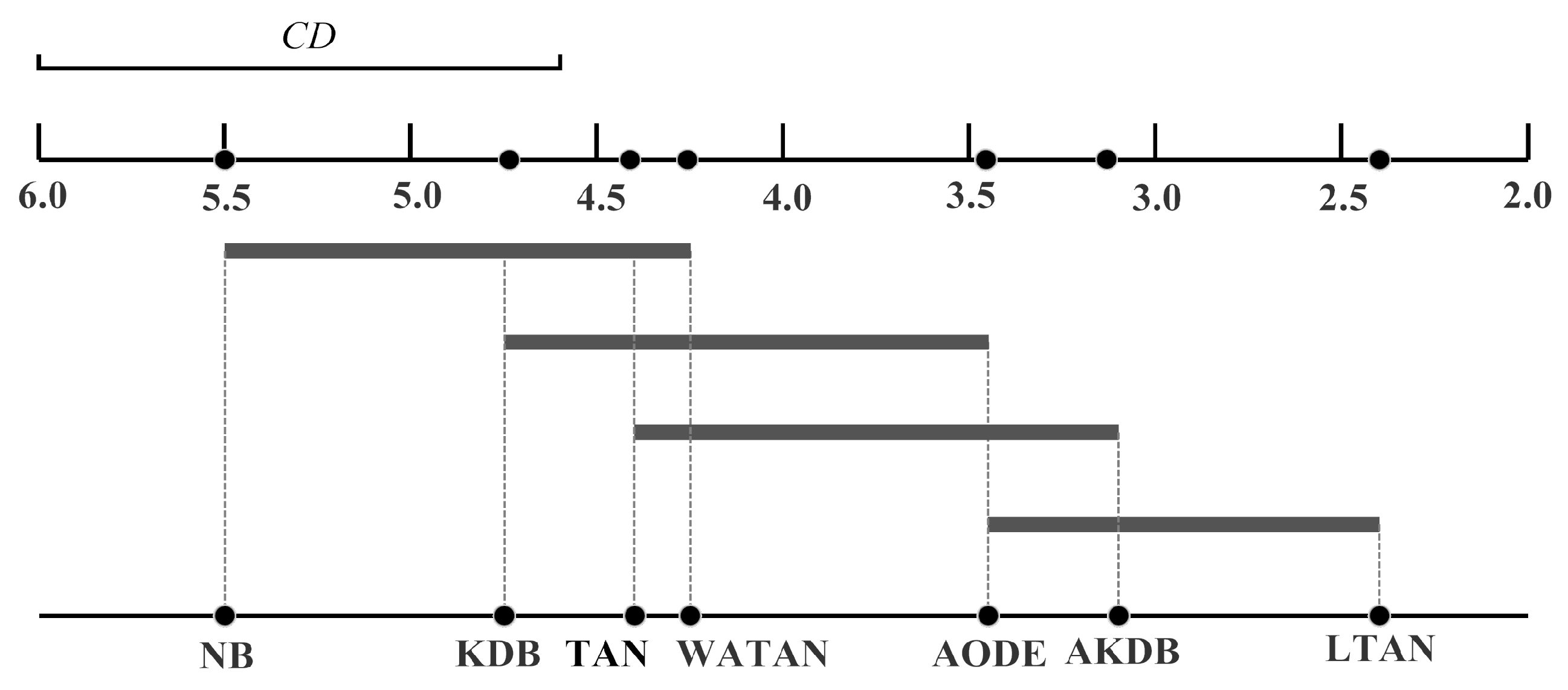
Figure 6.
The value of each dataset.

Figure 7.
Distribution of datasets whose values fall in a certain range.

Figure 8.
Comparisons of against per dataset.

Figure 9.
Distribution of datasets whose values fall in a certain range.

Figure 10.
Comparisons of l against per multi-class dataset.

Figure 11.
Zero-one loss comparisons between TAN and TAN per multi-class dataset.

Figure 12.
Comparisons of against per dataset.

Figure 13.
Time comparisons of TAN, LTAN and AKDB per dataset. TAN: tree-augmented naive Bayes. LTAN: label-driven TAN. AKDB: averaged k-dependence Bayesian classifier. (a) training time; (b) classification time.
Figure 13.
Time comparisons of TAN, LTAN and AKDB per dataset. TAN: tree-augmented naive Bayes. LTAN: label-driven TAN. AKDB: averaged k-dependence Bayesian classifier. (a) training time; (b) classification time.

Figure 14.
Network structures of TAN and E on the testing instance in Table 7: (a) TAN; (b) E.
Figure 14.
Network structures of TAN and E on the testing instance in Table 7: (a) TAN; (b) E.

Table 1.
Two testing instances in the Nursery dataset.
| No. | |
|---|---|
| 1 | |
| 2 |
Table 2.
The class membership probabilities of the testing instances in Table 1 estimated by TAN.
Table 2.
The class membership probabilities of the testing instances in Table 1 estimated by TAN.
| No. | |||||||
|---|---|---|---|---|---|---|---|
| 1 | 2.8394×10 | 1.7242×10 | 5.8891×10 | 1.2269×10 | 0.9984 | ||
| 2 | 3.9812×10 | 2.5073×10 | 5.3492×10 | 0.5051 | 0.4945 |
is a TAN model, is the label predicted by and is the true label of x.
Table 3.
Datasets.
| No. | Dataset | Instance | Att. | Class | No. | Dataset | Instance | Att. | Class |
|---|---|---|---|---|---|---|---|---|---|
| 1 | Lung Cancer | 32 | 56 | 3 | 21 | Segment | 2310 | 19 | 7 |
| 2 | Labor-negotiations | 57 | 16 | 2 | 22 | Hypothyroid | 3163 | 25 | 2 |
| 3 | Post-operative | 90 | 8 | 3 | 23 | Kr-vs-Kp | 3196 | 36 | 2 |
| 4 | Zoo | 101 | 16 | 7 | 24 | Hypo | 3772 | 29 | 4 |
| 5 | Promoters | 106 | 57 | 2 | 25 | Waveform-5000 | 5000 | 40 | 3 |
| 6 | Iris | 150 | 4 | 3 | 26 | Phoneme | 5438 | 7 | 50 |
| 7 | Teaching-ae | 151 | 5 | 3 | 27 | Page-blocks | 5473 | 10 | 5 |
| 8 | Sonar | 208 | 60 | 2 | 28 | Optdigits | 5620 | 64 | 10 |
| 9 | Heart | 270 | 13 | 2 | 29 | Mushrooms | 8124 | 22 | 2 |
| 10 | Hungarian | 294 | 13 | 2 | 30 | Thyroid | 9169 | 29 | 20 |
| 11 | Heart-disease-c | 303 | 13 | 2 | 31 | Pendigits | 10,992 | 16 | 10 |
| 12 | Dermatology | 366 | 34 | 6 | 32 | Sign | 12,546 | 8 | 3 |
| 13 | Musk1 | 476 | 166 | 2 | 33 | Nursery | 12,960 | 8 | 5 |
| 14 | Cylinder-bands | 540 | 39 | 2 | 34 | Letter-recog | 20,000 | 16 | 26 |
| 15 | Chess | 551 | 39 | 2 | 35 | Shuttle | 58,000 | 9 | 7 |
| 16 | Syncon | 600 | 60 | 6 | 36 | Waveform | 100,000 | 21 | 3 |
| 17 | Soybean | 683 | 35 | 19 | 37 | Census-income | 299,285 | 41 | 2 |
| 18 | Breast-cancer-w | 699 | 9 | 2 | 38 | Covtype | 581,012 | 54 | 7 |
| 19 | Tic-Tac-Toe | 958 | 9 | 2 | 39 | Poker-hand | 1,025,010 | 10 | 10 |
| 20 | Vowel | 990 | 13 | 11 | 40 | Donation | 5,749,132 | 11 | 2 |
Table 4.
Experimental results of zero-one loss.
| No. | Dataset | LTAN | NB | TAN | KDB | AODE | WATAN | AKDB |
|---|---|---|---|---|---|---|---|---|
| 1 | Lung Cancer | 0.5938 | 0.4375 | 0.5938 | 0.5938 | 0.4688 | 0.6250 | 0.6562 |
| 2 | Labor-negotiations | 0.0702 ∘ | 0.0702 | 0.1053 | 0.0351 | 0.0526 | 0.1053 | 0.0702 |
| 3 | Post-operative | 0.3444 ∘ | 0.3444 | 0.3667 | 0.3444 | 0.3444 | 0.3667 | 0.3333 |
| 4 | Zoo | 0.0099 | 0.0297 | 0.0099 | 0.0495 | 0.0198 | 0.0198 | 0.0297 |
| 5 | Promoters | 0.0849 ∘ | 0.0755 | 0.1321 | 0.1321 | 0.1038 | 0.1132 | 0.0943 |
| 6 | Iris | 0.0867 • | 0.0867 | 0.0800 | 0.0867 | 0.0867 | 0.0800 | 0.0867 |
| 7 | Teaching-ae | 0.5099 ∘ | 0.4967 | 0.5497 | 0.5430 | 0.4570 | 0.5364 | 0.5033 |
| 8 | Sonar | 0.2115 | 0.2308 | 0.2212 | 0.2308 | 0.2260 | 0.2212 | 0.2212 |
| 9 | Heart | 0.1778 ∘ | 0.1778 | 0.1926 | 0.1963 | 0.1704 | 0.1926 | 0.2037 |
| 10 | Hungarian | 0.1565 ∘ | 0.1599 | 0.1701 | 0.1701 | 0.1667 | 0.1735 | 0.1497 |
| 11 | Heart-disease-c | 0.1980 | 0.1815 | 0.2079 | 0.2079 | 0.1947 | 0.2046 | 0.2013 |
| 12 | Dermatology | 0.0137 ∘ | 0.0191 | 0.0328 | 0.0301 | 0.0219 | 0.0328 | 0.0219 |
| 13 | Musk1 | 0.1071 ∘ | 0.1660 | 0.1134 | 0.1113 | 0.1366 | 0.1134 | 0.1071 |
| 14 | Cylinder-bands | 0.1704 ∘ | 0.2148 | 0.2833 | 0.2278 | 0.1889 | 0.2463 | 0.2148 |
| 15 | Chess | 0.0980 • | 0.1125 | 0.0926 | 0.0998 | 0.1053 | 0.0926 | 0.0998 |
| 16 | Syncon | 0.0117 • | 0.0283 | 0.0083 | 0.0100 | 0.0133 | 0.0083 | 0.0150 |
| 17 | Soybean | 0.0425 ∘ | 0.0893 | 0.0469 | 0.0644 | 0.0542 | 0.0527 | 0.0498 |
| 18 | Breast-cancer-w | 0.0372 ∘ | 0.0258 | 0.0415 | 0.0486 | 0.0386 | 0.0415 | 0.0300 |
| 19 | Tic-Tac-Toe | 0.2328 | 0.3069 | 0.2286 | 0.2463 | 0.2683 | 0.2265 | 0.2683 |
| 20 | Vowel | 0.1394 • | 0.4242 | 0.1303 | 0.2343 | 0.1747 | 0.1263 | 0.2182 |
| 21 | Segment | 0.0364 ∘ | 0.0788 | 0.0390 | 0.0403 | 0.0329 | 0.0394 | 0.0385 |
| 22 | Hypothyroid | 0.0092 ∘ | 0.0149 | 0.0104 | 0.0107 | 0.0130 | 0.0104 | 0.0092 |
| 23 | Kr-vs-Kp | 0.0576 ∘ | 0.1214 | 0.0776 | 0.0544 | 0.0854 | 0.0776 | 0.0507 |
| 24 | Hypo | 0.0130 ∘ | 0.0138 | 0.0141 | 0.0077 | 0.0106 | 0.0130 | 0.0087 |
| 25 | Waveform-5000 | 0.1630 ∘ | 0.2006 | 0.1844 | 0.1820 | 0.1462 | 0.1844 | 0.1644 |
| 26 | Phoneme | 0.2378 ∘ | 0.2615 | 0.2733 | 0.2120 | 0.2100 | 0.2345 | 0.1885 |
| 27 | Page-blocks | 0.0369 ∘ | 0.0619 | 0.0415 | 0.0433 | 0.0322 | 0.0418 | 0.0347 |
| 28 | Optdigits | 0.0345 ∘ | 0.0767 | 0.0407 | 0.0416 | 0.0278 | 0.0406 | 0.0400 |
| 29 | Mushrooms | 0.0001 | 0.0196 | 0.0001 | 0.0006 | 0.0002 | 0.0001 | 0.0006 |
| 30 | Thyroid | 0.0681 ∘ | 0.1111 | 0.0720 | 0.0693 | 0.0719 | 0.0723 | 0.0674 |
| 31 | Pendigits | 0.0225 ∘ | 0.1181 | 0.0321 | 0.0362 | 0.0187 | 0.0328 | 0.0286 |
| 32 | Sign | 0.2659 | 0.3586 | 0.2755 | 0.2881 | 0.2822 | 0.2752 | 0.2826 |
| 33 | Nursery | 0.0590 ∘ | 0.0973 | 0.0654 | 0.0654 | 0.0733 | 0.0654 | 0.0633 |
| 34 | Letter-recog | 0.1043 ∘ | 0.2525 | 0.1300 | 0.1285 | 0.0863 | 0.1300 | 0.1203 |
| 35 | Shuttle | 0.0009 ∘ | 0.0039 | 0.0015 | 0.0015 | 0.0011 | 0.0014 | 0.0010 |
| 36 | Waveform | 0.0195 | 0.0220 | 0.0202 | 0.0226 | 0.0180 | 0.0202 | 0.0200 |
| 37 | Census-income | 0.0542 ∘ | 0.2363 | 0.0628 | 0.0619 | 0.1013 | 0.0628 | 0.0513 |
| 38 | Covtype | 0.2378 ∘ | 0.3158 | 0.2517 | 0.2451 | 0.2385 | 0.2516 | 0.2445 |
| 39 | Poker-hand | 0.2266 ∘ | 0.4988 | 0.3295 | 0.3291 | 0.4812 | 0.3295 | 0.0763 |
| 40 | Donation | 0.0000 | 0.0002 | 0.0000 | 0.0000 | 0.0002 | 0.0000 | 0.0000 |
LTAN: label-driven tree-augmented naive Bayes. NB: naive Bayes. TAN: tree-augmented naive Bayes. KDB: k-dependence Bayesian classifier. AODE: averaged one-dependence estimators. WATAN: weighted averaged TAN. AKDB: averaged KDB. ∘, • denote significant improvement or degradation of LTAN over TAN. All results are rounded to four decimal places.
Table 5.
Win/Draw/Loss records of zero-one loss on all datasets.
| W/D/L | NB | TAN | KDB | AODE | WATAN | AKDB |
|---|---|---|---|---|---|---|
| TAN | 26/3/11 | |||||
| KDB | 26/4/10 | 7/22/11 | ||||
| AODE | 28/7/5 | 21/4/15 | 20/8/12 | |||
| WATAN | 28/1/11 | 5/33/2 | 13/20/7 | 13/7/20 | ||
| AKDB | 27/7/6 | 21/9/10 | 20/15/5 | 16/8/16 | 22/10/8 | |
| LTAN | 30/6/4 | 27/9/4 | 26/9/5 | 22/6/12 | 25/11/4 | 18/15/7 |
Significant () win/draw/loss records are shown in bold.
Table 6.
Datasets where the classification accuracy of LTAN degrades significantly compared to TAN.
| No. | Dataset | Instance | Class | ||
|---|---|---|---|---|---|
| 1 | Iris | 150 | 3 | 0.00% | 7.14% |
| 2 | Chess | 551 | 2 | 4.05% | 5.41% |
| 3 | Syncon | 600 | 6 | 0.00% | 66.67% |
| 4 | Vowel | 900 | 11 | 7.09% | 10.14% |
Table 7.
A testing instance in Vowel which is misclassified by LTAN but correctly classified by TAN.
Table 7.
A testing instance in Vowel which is misclassified by LTAN but correctly classified by TAN.
| x = (1,14,1, (−2.3195,−2.1045], >3.1765, ≤0.4725, ≤−0.0225, (−0.7345,0.4995], ≤1.2250, (−1.1270,−0.6575], (−0.5970,0.1185], ≤−0.9465,known) |
Numerical attributes are discretized using MDL. is the true label of x.
Table 8.
The class membership probabilities of the testing instance in Table 7 estimated by TAN, TAN, IBMC and LTAN.
Table 8.
The class membership probabilities of the testing instance in Table 7 estimated by TAN, TAN, IBMC and LTAN.
| Classifier | |||
|---|---|---|---|
| TAN | 0.7783 | 0.1691 | |
| TAN | 0.8215 | 0.1785 | |
| IBMC | 0.0185 | 0.9815 | |
| LTAN | 0.4200 | 0.5800 |
is a classifier, is the label predicted by . For TAN, only posterior probabilities of and are shown. After the label filtering, only and remain.
© 2017 by the authors. Licensee MDPI, Basel, Switzerland. This article is an open access article distributed under the terms and conditions of the Creative Commons Attribution (CC BY) license (http://creativecommons.org/licenses/by/4.0/).
Share and Cite
MDPI and ACS Style
Sun, Y.; Wang, L.; Sun, M. Label-Driven Learning Framework: Towards More Accurate Bayesian Network Classifiers through Discrimination of High-Confidence Labels. Entropy 2017, 19, 661. https://doi.org/10.3390/e19120661
AMA Style
Sun Y, Wang L, Sun M. Label-Driven Learning Framework: Towards More Accurate Bayesian Network Classifiers through Discrimination of High-Confidence Labels. Entropy. 2017; 19(12):661. https://doi.org/10.3390/e19120661
Chicago/Turabian StyleSun, Yi, Limin Wang, and Minghui Sun. 2017. "Label-Driven Learning Framework: Towards More Accurate Bayesian Network Classifiers through Discrimination of High-Confidence Labels" Entropy 19, no. 12: 661. https://doi.org/10.3390/e19120661
Note that from the first issue of 2016, this journal uses article numbers instead of page numbers. See further details here.