Tsallis Entropy Theory for Modeling in Water Engineering: A Review


1
Department of Biological and Agricultural Engineering, Texas A&M University, College Station, TX 77843-2117, USA
2
Zachry Department of Civil Engineering, Texas A&M University, College Station, TX 77843-2117, USA
3
School of Civil and Environmental Engineering, The University of New South Wales, Sydney, NSW 2052, Australia
4
Department of Land, Air and Water Resources, University of California, Davis, CA 95616, USA
5
Key Laboratory of Land Surface Pattern and Simulation, Institute of Geographic Sciences and Natural Resources Research, Chinese Academy of Sciences, Beijing 100101, China
*
Authors to whom correspondence should be addressed.
Entropy 2017, 19(12), 641; https://doi.org/10.3390/e19120641
Submission received: 15 September 2017
/
Revised: 15 November 2017
/
Accepted: 23 November 2017
/
Published: 27 November 2017
(This article belongs to the Special Issue Entropy Applications in Environmental and Water Engineering)
Abstract
:Water engineering is an amalgam of engineering (e.g., hydraulics, hydrology, irrigation, ecosystems, environment, water resources) and non-engineering (e.g., social, economic, political) aspects that are needed for planning, designing and managing water systems. These aspects and the associated issues have been dealt with in the literature using different techniques that are based on different concepts and assumptions. A fundamental question that still remains is: Can we develop a unifying theory for addressing these? The second law of thermodynamics permits us to develop a theory that helps address these in a unified manner. This theory can be referred to as the entropy theory. The thermodynamic entropy theory is analogous to the Shannon entropy or the information theory. Perhaps, the most popular generalization of the Shannon entropy is the Tsallis entropy. The Tsallis entropy has been applied to a wide spectrum of problems in water engineering. This paper provides an overview of Tsallis entropy theory in water engineering. After some basic description of entropy and Tsallis entropy, a review of its applications in water engineering is presented, based on three types of problems: (1) problems requiring entropy maximization; (2) problems requiring coupling Tsallis entropy theory with another theory; and (3) problems involving physical relations.
1. Introduction
Water resources systems serve a multitude of human needs. They are needed for water supply, water transfer, water diversion, irrigation, land reclamation, drainage, flood control, hydropower generation, river training, navigation, coastal protection, pollution abatement, transportation and recreation, among others. Many of the systems (e.g., channels, culverts, impoundments) have been with us since the birth of human civilization. Some (e.g., spillways, small dams, levees) are several centuries old, while some others (e.g., large dams, long-distance water transfer structures) are of more recent origin. In the beginning, systems were designed more or less empirically. Then, engineering and economics constituted the sole foundation of design. About fifty years ago, planning and design of hydraulic structures went through a dramatic metamorphosis. These days, they are based on both engineering and non-engineering aspects. Engineering aspects encompass planning, development, design, operation and management, while non-engineering aspects include environmental impact assessment, socio-economic analysis, policy making and impact on society.
For designing water engineering systems (e.g., channels, levees, bridge piers, drainage structures, dams, reservoirs, spillways), some key questions that need to be addressed relate to the following, among others: peak discharge; velocity distribution; sediment yield, concentration and discharge; pollutant load, concentration and transport; river bed profile, meandering and braiding; downstream and at-a-point hydraulic geometry; flow depth, discharge and velocity routing; and seepage through a dam. For water supply systems, the key questions are concerned with, among others: reliability; loss of energy in the distribution system; and pipe sizes. In addition, pollutant concentration and transport as well as pollution abatement are also now considered as essential components of water resources system design. In a similar manner, because of increased public awareness, primarily triggered by environmental movement, non-engineering aspects of hydraulic design, dubbed under “socio-economic analyses,” play a critical role. Besides engineering feasibility and economic viability, issues related to public health, political support, legal and judicial restrictions and social acceptability determine, to a large extent, if the water resources project will go off the ground.
A survey of the water engineering literature shows that there are myriad techniques for addressing questions pertaining to the design of water resources systems. The techniques range from empirical to semi-empirical to physically-based ones. Empirical techniques are data-based; examples are regression, time series analysis and other statistical methods. Semi-empirical methods, also sometimes referred to as conceptual or systems-based techniques, employ mass conservation and some empirical relationship or hypothesis; a good example is the unit hydrograph theory. Physically-based methods employ the laws of conservation of mass, momentum and energy; an example is the use of St. Venant’s equations for flow routing or Richards’ equation for computing infiltration. Strictly speaking, even physically-based methods also employ empirical parameters and, thus, are not entirely “physically-based.” Indeed, all these three types of techniques employ some physics through data or hypotheses or laws. Extensive details of these methods are already well-documented in the literature [1,2,3,4,5,6]. A more recent and comprehensive account of these methods and applications is also presented in [7].
Because of the large diversity of these techniques, based on different hypotheses and assumptions, it is difficult to present the developments in any subject or field of interest in a unified and coherent manner. This becomes particularly challenging when undertaking water resources system engineering design. There are, of course, some theories that do apply to a wide variety of problems, such as kinematic wave theory and diffusion wave theory [8,9]. These theories can be applied to solve a wide variety of problems where the movement of water, sediment and/or pollutant is involved. However, many problems in water engineering design require a statistical treatment. For addressing such problems, entropy theory can serve as a unifying theory. During the past three decades, entropy theory has been applied to address a wide spectrum of problems in water engineering, including rainfall-runoff [1,3,8], infiltration [2], soil moisture [2], network design [10], velocity distributions [11,12,13,14], sediment concentration and discharge [15,16,17], hydraulic geometry [18,19,20,21,22] and reliability [23], among others. For recent comprehensive accounts of entropy theory applications in water and environmental engineering, see [24,25,26].
The origin of entropy theory is in the second law of thermodynamics. Koutsoyiannis [27] has presented a nice account of the historical background of entropy. The most commonly used measure of entropy is the Boltzmann-Gibbs-Shannon (BGS) entropy [28], which is often referred simply as the Shannon entropy [29]. Tsallis [30] introduced a more general entropy function for complex systems, which is now referred to as the Tsallis entropy. Tsallis entropy specializes in the Shannon entropy. During the last two decades or so, Tsallis entropy theory has found many applications in water and environmental engineering and there is certainly a great potential to extend the applications to a much wider spectrum of water systems and associated problems.
This paper aims to provide a review of the applications of Tsallis entropy theory in water engineering. It revisits the Tsallis entropy theory, presents a general methodology for application of the theory, shows how entropy theory couples statistical information with physical laws and how it can be employed to derive useful physical constructs in time and/or space and provides a review of physical applications of the Tsallis entropy theory in water engineering.
The rest of the paper is organized as follows. Section 2 reviews the Tsallis entropy theory. Section 3, Section 4, Section 5 and Section 6 review the applications of the Tsallis entropy theory in water engineering. Section 3 presents an overview of three types of problems in water engineering. Section 4 reviews problems requiring entropy maximization. Section 5 reviews coupling entropy theory with another theory. Section 6 reviews physical relations. Section 7 draws some conclusions.
2. Tsallis Entropy Theory
2.1. Definition of Entropy
The concept of entropy is closely linked with the concept of uncertainty, information, chaos, disorder, surprise or complexity. Indeed, there are often different interpretations of entropy in different fields [24,25,26,31,32,33]. For instance, in statistics, entropy is regarded as a measure of randomness, objectivity or unbiasedness, dependence, or departure from the uniform distribution. In ecology, it is a measure of diversity of species or lack of concentration. In water engineering, it is a measure of information of uncertainty. In industrial engineering, it is a measure of complexity. In manufacturing, it is a measure of interdependence. In management, it is a measure of similarity. In social sciences, it is measure of equality. This may be illustrated as follows.
Consider a random variable X that takes on values that occur with probabilities If pi = 1 (the event is certain to occur), pj = 0 (the event is certain not to occur), then it can be said that there is no surprise about the occurrence or non-occurrence of event X = xi and the occurrence or non-occurrence of this event provides no information. The system that produces such an event has no complexity and is not chaotic or disorderly. On the other hand, if an event xi occurs with very small probability pi, say 0.01, then our anticipation of event xi is highly uncertain and if xi does indeed occur, then there will be a great deal of surprise about its occurrence. The occurrence of this event provides a great deal of information and the system producing such an event is complex, chaotic and disorderly. Intuitively, the information content of event xi or the anticipatory uncertainty of xi prior to the observation decreases as the value of probability p(xi) increases [24,26]. It may be noted that information is gained only if the variable takes on different values. The value that occurs with a higher probability conveys less information and vice versa.
It is logical to deduce that if a system has more uncertainty, then more information will be needed to characterize it and vice versa. That is, information reduces uncertainty, meaning that, for a system, more information means less uncertainty. Uncertainty increases the need for more information; that is, more uncertainty means more information is needed. Shannon [29] formulated entropy as the expected value of the probabilities of values that a variable or event may take on. The information gained is indirectly measured as the amount of reduction of uncertainty. Thus, entropy is defined as a measure of disorder, chaos, uncertainty, surprise, or information.
From an informational perspective, the information gain from the occurrence of any event xi, can be expressed as:
Equation (1) says that the information gained is minus the logarithm of the inverse of the probability of occurrence. For N events, the average or expected information gain, Hs, is the weighted average of Equation (1):
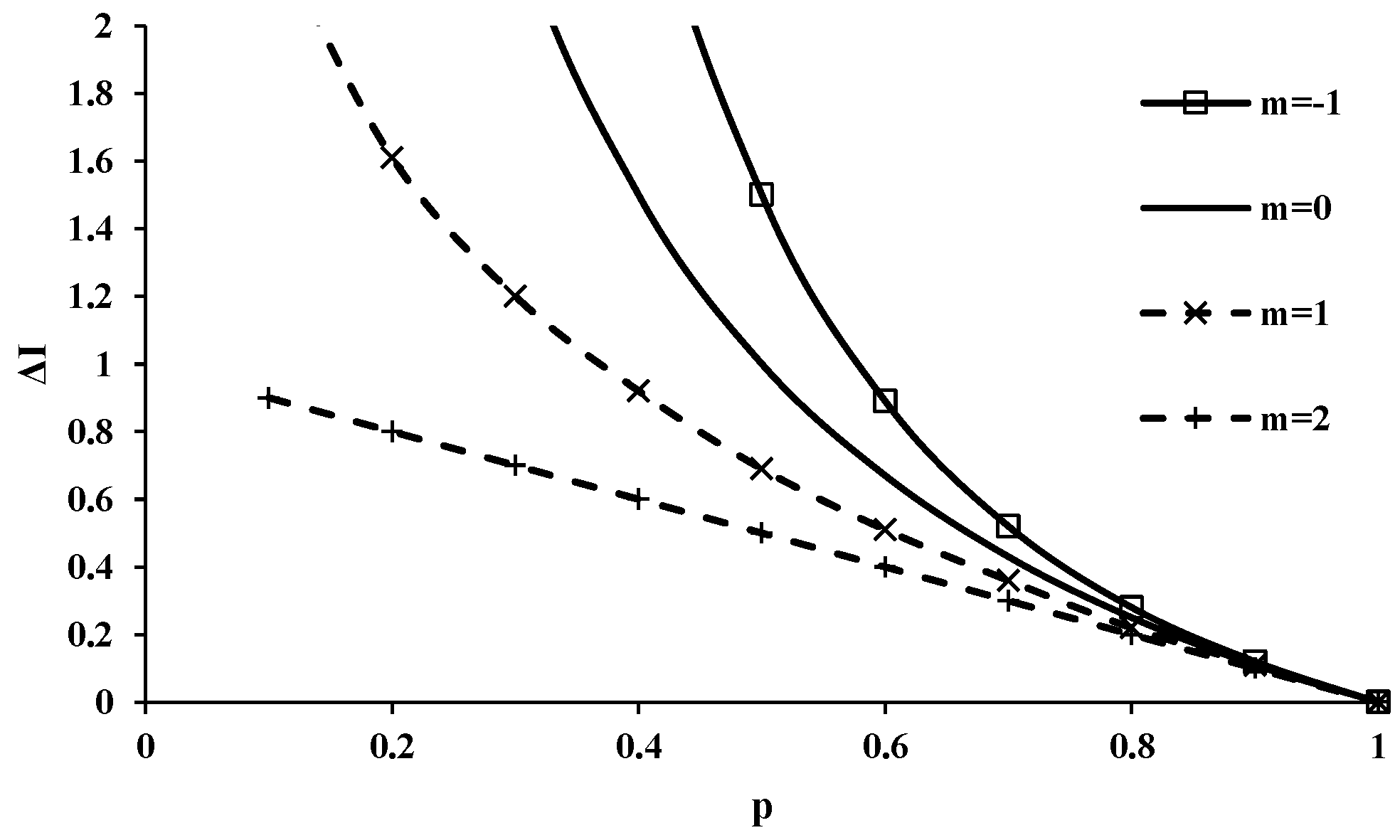
Equation (2) is the Shannon entropy [29], also called informational entropy. Equation (1) shows that the information gain is directly a function of probability and is, hence, called gain function. Equation (1) can be generalized by expressing it as a power function, given by:
where ΔI(xi) is the gain in information from an event i which occurs with probability pi and m is any real number. The gain function computed from Equation (3) for m = −1, 0, 1 and 2, as shown in Figure 1, decreases with an increase in the probability value regardless of the value of m. For increasing value of m, the gain function diminishes for the same probability value. The gain function has a much longer tail, showing very low values of gain as the probability increases.
Analogous to Shannon entropy, the average or expected gain function for N events, Hm, is the weighted average of Equation (3), given by:
where Hm is designated as the Tsallis entropy or m-entropy [30], which is often referred to as the non-extensive statistic, m-statistic, or Tsallis statistic. It can be shown that as Tsallis entropy converges to Shannon entropy. The quantity m is often referred to as the non-extensivity index, Tsallis entropy index, or simply entropy index and its value can be positive or negative. Entropy index m reflects the microscopic dynamics and the degree of nonlinearity of the system. Since almost all real systems (e.g., water systems) are inherently nonlinear in nature, the Tsallis entropy has a clear advantage when compared to the Shannon entropy. Tsallis [34] noted that super-extensivity, extensivity and sub-extensivity occur when m < 1, m = 1 and m > 1, respectively. Interestingly, if corresponds to the rare events and m > 1 corresponds to frequent events [35,36], pointing to the stretching or compressing of the entropy curve to lower or higher maximum entropy positions.
If random variable X is non-negative continuous with a probability density function (PDF), f(x), then the Shannon entropy can be written as:
From now onwards, subscript m will be deleted and Hm will be simply denoted by H.
A plot of H versus p for m = −1, −0.5, 0, 0.5, 1 and 2 is given in Figure 2. For m < 0, the Tsallis entropy is concave; and for m > 0, it becomes convex. For m = 0, H = (N − 1) for all pi’s. For m = 1, it converges to Shannon entropy. For all cases, the Tsallis entropy decreases as m increases.
2.2. Properties of Tsallis Entropy
As mentioned earlier, the concept of entropy is closely linked with the concept of uncertainty, information, chaos, disorder, surprise or complexity. Tsallis entropy has some interesting properties [30,40] that are briefly summarized here.
(1) m-entropy: The m-surprise or m-unexpectedness is defined as logm(1/pi), where the logarithm is the base m. Hence, the m-entropy can be defined as:
which coincides with the Tsallis entropy:
in which E is the expectation.
(2) Maximum value: Equation (4) attains an extreme value for all values of m when all pi’s are equal, i.e., pi = 1/N. For m > 0, it attains a maximum value and for m < 0 it attains a minimum value. The extremum of H becomes
(3) Concavity: For two probability distributions and corresponding to a unique set of N possibilities, an intermediate probability distribution can be defined for a real a, such that 0 < a < 1, as:
for all i’s. It can be shown that for m > 0,
and for m < 0,
Functional if m > 0 and is, hence, concave; H(G) = 0 if m = 0; and if m < 0 and is, therefore, convex.
(4) Additivity: For two independent systems A and B with ensembles of configurational possibilities with probability distribution and configurational possibilities with probability distribution one can express the union of two systems and their corresponding ensembles of possibilities If represents the corresponding probabilities, then, by virtue of independence, the joint probability will be equal to the product of individual probabilities, i.e., or , for all i and j. One can write the entropy of the union of two systems A and B as:
Equation (13) describes the additivity property, which can be extended to any number of systems. In all cases, (non-negativity property). If systems A and B are correlated, then
for all (i, j). One may define mutual information of the two systems or transinformation S as:
Considering Equation (15), T(pij) = 0 for all m, if A and B are independent and Equation (15) will reduce to Equation (13). For correlated A and B, T(pij) < 0 for m = 1 and for m = 0. For arbitrary values of m, it will be sensitive to pij; it can take on negative or positive values for both m < 1 and m > 1 with no particular regularity and can exhibit more than one extremum.
(5) Composability: The entropy H(A + B) of a system comprised of two sub-systems A and B can be computed from the entropies of sub-systems, H(A) and H(B) and the entropy index m.
(6) Interacting sub-systems: Consider a set of N possibilities arbitrarily separated into two sub-systems with W1 and W2 possibilities, where W = W1 + W2. Defining and , , it can be shown that
where and are the conditional probabilities. Note that for m < 1 and for m > 1. Hence, m < 1 corresponds to rare events and m > 1 to frequent events [41]. This property can be extended to any number R of interacting sub-systems: Then, defining , Equation (16) can be generalized as:
Here,
2.3. Principle of Maximum Entropy
Quite often, some information may be known about the random variable X. Then, it seems logical to choose a PDF of X that is consistent with the known information. Since there can be more than one PDF that may satisfy this condition, Jaynes [42,43] formulated the principle of maximum entropy (POME), which states that one should choose the distribution that has the highest entropy, subject to the given information. This distribution will be the least-biased distribution. Furthermore, it is equivalent to the minimum relative (cross) entropy condition when no prior is given, which is also called as the Kullback-Leibler principle [44]. The implication here is that POME takes into account all of the given information and, at the same time, avoids consideration of any information that is not given. This is consistent with Laplace’s principle of insufficient reason (or principle of indifference), according to which all outcomes of an experiment should be considered equally likely unless there is information to the contrary. Therefore, POME enables entropy theory to achieve the probability distribution of a given random variable.
The procedures for applications of POME entails the following steps [24,26]: (1) definition of Tsallis entropy; (2) specification of constraints; (3) maximization of entropy, in accordance with POME, using of the method of Lagrange multipliers; (4) derivation of the probability distribution in terms of constraints; (5) determination of Lagrange multipliers; and (6) determination of the maximum entropy. Since the definition of entropy has already been reviewed earlier, it will not be repeated here. The remaining steps, (2)–(6), are briefly discussed here.
2.3.1. Specification of Constraints
For deriving the PDF of a random variable X using POME, appropriate constraints need to be defined. Papalexiou and Koutsoyiannis [28] suggested three considerations for defining constraints: (1) Simplicity and physical meaningfulness; (2) little variability in the future; and (3) definition in terms of laws of physics—mass, momentum and energy conservation and constitutive laws—as far as possible. For simplicity, constraints are often defined in terms of statistical moments and, fortunately, the moments are related to the laws of physics.
Let Ci denote the i-th constraint, i = 0, 1, 2, …, n, where n is the number of constraints. Let gr(x) be an arbitrary function of X. Then, constraints Cr, r = 0, 1, 2, …, n, can be defined as:
where g0(x) = 0; gr(x), r = 1, 2, …, n, represents some function of x and is the expectation of gr(x). Equation (18) states the total probability theorem that the PDF must satisfy. If r = 1 (first moment) and g1(x) = x, then Equation (19) represents the mean ; likewise, for r = 2 (second moment) and , it denotes the variance (σ2) of X. The first moment corresponds to the conservation of mass and the second moment to the conservation of momentum. Similarly, r = 3 (third moment), measuring skewness, corresponds to the conservation of energy. It is noticed that the order of moments higher than 3 may be unreliable [45]. In water engineering, two or three constraints usually suffice.
2.3.2. Entropy Maximizing Using Lagrange Multipliers
Tsallis entropy, given by Equation (6), can be maximized, subject to constraints defined by Equations (18) and (19), using the method of Lagrange multipliers [42,43]. Therefore, the Lagrangian function L can be expressed as:
where λi, i = 0, 1, 2, …, M, are the Lagrange multipliers. Note that −1/(m − 1) is added to the zeroth Lagrange multiplier for algebraic simplification. Using the Euler-Lagrange calculus of variation, differentiating Equation (20) with respect to f(x) and equating the derivative to zero, we obtain:
2.3.3. Determination of Probability Distribution
Equation (21) yields the least-biased probability distribution of X:
Integrating Equation (22), the cumulative distribution function F(x) is obtained as:
The properties of the probability distribution will depend on the value of m, Lagrange multipliers, functions gi(x) and M.
2.3.4. Determination of the Lagrange Multipliers
Equation (22) contains M unknown Lagrange multipliers that can be determined with the use of Equations (18) and (19). Substituting Equation (22) in Equations (18) and (19), the result is, respectively:
Solution of Equations (24) and (25) yields the unknown Lagrange multipliers It may be noted from Equation (24) that λ0 can be expressed as a function of other Lagrange multipliers and, therefore, the unknown multipliers are λi, i = 1, 2, …, M. Except for simple cases, Equations (24) and (25) do not have an analytical solution but can be solved numerically.
2.3.5. Determination of Maximum Entropy
Substitution of Equation (24) in Equation (6) leads to the maximum Tsallis entropy:
Equation (26) shows that the entropy of the probability distribution of X depends only on the specified constraints, since the Lagrange multipliers themselves can be expressed in terms of the specified constraints.
3. Applications in Water Engineering: Overview
The problems that can be addressed using the Tsallis entropy theory can be classified into three groups. The first group consists of problems that only require the maximization of the Tsallis entropy, which can be accomplished using POME. Examples of such problems include frequency analysis, parameter estimation, network evaluation and design, spatial and inverse spatial analysis, geomorphologic analysis, grain size distribution analysis, flow forecasting, complexity analysis and clustering [46,47,48,49,50,51,52].
The types of problems included in the second group require coupling with another theory, such as the theory of stream power or theory of minimum energy dissipation rate. Examples of problems in this group include hydraulic geometry [19,20] and evaporation [53]. Also included in this group are problems wherein first relations between entropy and design variables are derived and then relations between design variables and system characteristics are established. Examples include geomorphologic relations for elevation, slope and fall; and evaluation of water distribution systems [54,55].
The third group includes problems that require deriving a physical relation either in time or in space. This means, the domain of analysis requires a shift from the probability domain to a real domain (space or time), which is accomplished by invoking a relation between the cumulative probability distribution function and the design variable. Examples of such problems are infiltration capacity, soil moisture movement in vadose zone, groundwater head distribution, velocity distribution, rainfall-runoff relation, channel geometry, rating curve, flow-duration curve, erosion and sediment yield, sediment concentration and discharge, debris flow, longitudinal river profile, hydraulic geometry, channel cross-section shape and rating curve [19,20,21,22,56,57,58,59,60,61]. The objective in this class of problems is to derive a relation of the design variable as a function of time or space.
These three kinds of problems are further detailed in the following sections, with examples from water engineering.
4. Problems Requiring Entropy Maximization
Fundamental to solving problems that only require entropy maximization is the derivation of probability distribution. A multitude of problems in water engineering involve essentially data analysis for deriving either a probability distribution or computing entropy.
4.1. Frequency Distributions
The procedure for deriving a maximum entropy-based frequency distribution has been discussed above. The procedure is illustrated here using only two constraints: mean (first moment) and second moment. For any probability density function, f(x), of a random variable X, the total probability must equal one, i.e.,
The first and second moments can be defined, respectively, as:
and
In order to obtain the least-biased f(x), subject to Equations (27)–(29), Equation (6) can be maximized for m > 0 using the method of Lagrange multipliers. The Lagrange function L can be written as:
Differentiating L with respect to f(x) and equating the derivative to zero, one obtains:
Equation (32) is the entropy-based probability density function of power type.
The Lagrange multipliers, λi, i = 0, 1, 2 and, consequently, , can be estimated using Equations (27) to (29). For simplification, let λ2 be assumed as 0. Then, Equation (32) becomes:
whose parameters are estimated using Equations (27) and (28). Substituting Equation (33) in Equation (27), one obtains:
or
The other Lagrange multiplier can be determined by inserting Equation (33) in Equation (28) and is given as:
By solving Equations (34) or (35) with (36), Lagrange multipliers α1 and α0 can be determined. Inserting Equation (34) in Equation (33), one obtains
Let
Using Equation (38), Equation (37) becomes
Equation (39) is a two-parameter generalized Pareto distribution.
Let
Equation (39) then becomes
Equation (41) is a two-parameter Pareto distribution. If k → 0, then Equation (41) leads to an exponential distribution:
Koutsoyiannis [37,38] proposed a generalization, following which Equation (32) can be expressed as:
where c1 and c2 are shape parameters. Equation (43) has four parameters: scale parameter α1 and shape parameters k and c1 and c2. Note that α0 is not a parameter, because it is a constant based on the satisfaction of Equation (27). It is, however, not clear as to what led to the generalized form of Equation (43). Koutsoyiannis [37] suggested that random variable would have Beta Prime (also referred to as Beta of the second kind) distribution [62]. Then, the distribution of X would be referred to as the power-transformed Beta Prime (PBP). Koutsoyiannis [37] showed that Equation (43) can specialize into several exponential and power-type probability distributions, such as PBP-L1 , gamma , Weibull , Pareto , Beta Prime , PBP-L2 and others.
4.2. Network Evaluation and Design
Hydrometric data are required for an efficient planning, design, development, operation and management of water engineering systems. Many studies have applied the Shannon entropy theory to assess and optimize data collection networks (e.g., water quality, rainfall, streamflow, hydrometric, elevation, landscape, etc.) [63,64] but not the Tsallis entropy theory. The basic idea for developing a methodology for data collection network design is that it must take into account the information of each gaging station or potential gaging station in the network. A station with a higher information content is given a higher priority over other stations that have lower information content but the information content of a station must be tempered with the degree of use. That is, a station that is used by one user might be given a lower priority than a station that has diverse uses.
A framework for network design or evaluation considers a range of factors, such as: (a) objectives of sampling; (b) variables to be sampled; (c) locations of measurement stations; (d) frequency of sampling; (e) duration of sampling; (f) uses and users of data; and (g) socio-economic considerations. A network design has two modes: (1) number of gages and their locations (space evaluation); and (2) time interval for measurement (time evaluation).
Let there be two stations A and B with ensembles of configurational possibilities with probability distribution and configurational possibilities with probability distribution Then, the union of the two stations and their corresponding ensembles of possibilities are If represents the corresponding probabilities, then the mutual information or transinformation S can be expressed as:
From Equation (44), T(pij) = 0 for all m, if X and Y are independent. For correlated X and Y, T(pij) < 0 for m = 1 and for m = 0. For arbitrary values of m, it will be sensitive to pij; it can take on negative or positive values for both m < 1 and m > 1 with no particular regularity and can exhibit more than one extremum.
4.3. Directional Information Transfer Index
By dividing by the marginal entropy, the mutual information T can be normalized [65] as:
where HLost is the amount of information lost. The ratio of T by H is called the Directional Information Transfer (DIT) index. Mogheir and Singh [66] called it as the Information Transfer Index (ITI). The DIT varies from zero to unity and denotes the fraction of information transferred from one station to another. A zero value of DIT corresponds to the case where sites are independent and, therefore, no information is transmitted. A value of unity for DIT corresponds to the case where sites are fully dependent and no information is lost. Since DITXY = T/H(X) is not the same as DITYX = T/H(Y), DIT is not symmetrical. The term DITXY describes the fractional information inferred by station X about station Y, whereas DITYX describes the fractional information inferred by station Y about station X. Between two stations, the station with the higher DIT should be given higher priority because of its greater capability in inferring (predicting) the information at other sites. The DIT can be applied for regionalization of the network or watersheds.
4.4. Reliability of Water Distribution Networks
A water distribution system can be designed by minimizing head losses, costs, risks and departures from specified values of water quantity, pressure and quality and also maximizing reliability [67]. Thus, it becomes a multi-objective optimization problem. However, it is not uncommon to formulate the design problem as a single-objective optimization problem, where the system capital and operational costs are minimized and, at the same time, the laws of hydraulics are satisfied and the targets of water quantity and pressure at demand nodes are met. Fundamental to either type of optimization is reliability [68,69,70].
To develop a Tsallis entropy-based redundancy measure of the network with N nodes, where the nodes may be considered to constitute sub-systems, the Tsallis entropy of a node j can now be expressed in terms of Wij as:
where m is the entropy index and is a real number and Sj is an entropic measure of redundancy at node j and is local redundancy. Maximizing Sj would maximize redundancy of node j and is equivalent to maximizing entropy at node j. The maximum value of Sj is achieved when all Wij’s or qij/Qj’s are equal. This occurs when all qij’s are equal. For the entire water distribution network, redundancy is a function of redundancies Sj’s of individual nodes in the network.
The overall network redundancy can be assessed in two ways. First, the network redundancy can be assessed by the relative importance of a link to its node and its importance recognized by qij/Qj. In this case, the redundancy is maximized at each node. It may, however, be noted that the network redundancy is not a sum of nodal redundancies. Second, the network redundancy can be assessed by the relative importance of a link to the total flow and its importance recognized by qij/Q0. Here, the proposition is that the importance of a link relative to the local flow is not as important as it is to the total flow. In this case too, the network redundancy is not a sum of nodal redundancies. In order to acknowledge the relative importance of a link to the entire network, the nodal redundancy Sj* can be expressed as:
It may be noted that Sj*, given by Equation (47), is similar to the Sj given by Equation (46). In this case too, the maximum value of Sj* will occur when the qij values are equal at the j-th node. It can also be shown that the maximum network redundancy will be achieved when all the qij values are equal. It may, however, be noted that
This is because,
Therefore, in the second approach, Equation (47) can be used in the spirit of Tsallis entropy or considering it via partial Tsallis entropy [36].
The network redundancy for N nodes is a function of redundancies of individual nodes, Sj’s, in the network. However, it will not be a simple summation of these nodal redundancies, because of the non-extensive property of the Tsallis entropy. For the first approach, it can be shown that the network redundancy (with N nodes) can be expressed as:
In order to develop an appreciation for Equation (47), it will be instructive to expand Equation (47) in terms of flow quantities. Equation (47) is just the sum of nodal redundancies.
For the second approach, the network redundancy (with N nodes: 1, 2, …, N) can be expressed as:
It can be seen that Equation (51) for network redundancy with the second approach is significantly different from Equation (50) with the first approach.
5. Problems Requiring Coupling with another Theory
There are some problems where the entropy theory can only be part of the solution methodology and needs to be coupled with another theory. Consider, for example, hydraulic geometry of a river or channel, which is defined by the relations between discharge and each of hydraulic variables (e.g., flow width, depth, velocity under bankfull conditions) and each of geometric variables (e.g., bed roughness, slope). Hydraulic geometry is of two types: (1) downstream; and (2) at-a-point. For either type, the values of hydraulic and geometric variables are average annual values corresponding to the equilibrium or stable condition of the river. At this condition, the river will try to spend the least amount of energy for transporting water and sediment. In response to the influx of water and sediment coming from the watershed, the river will adjust these variables or characteristics in order to attain the stable condition. This means, the river will spread the adjustment as equitably as the environment will allow and will follow the theory of minimum energy dissipation rate. The equal rate of adjustment can be described by the principle of maximum entropy (POME) that the river will follow. In this manner, the theory of minimum energy dissipation rate and entropy theory are combined for determining the hydraulic geometry of a river or designing a stable canal. The advantage of the entropy theory is that it explicitly allows to incorporate the constraints imposed by the watershed and the design. For example, if a river is leveed, then it cannot adjust its width and the adjustment will be shared by depth and velocity. Likewise, if a canal is lined, it cannot adjust its width, slope and roughness and will have to adjust its depth and velocity. In this manner, a whole hierarchy of hydraulic geometry relations can be obtained, depending on the constraints imposed. The other existing theories do not allow this flexibility. In what follows, some specific examples of problems requiring coupling entropy theory with other theories are presented.
5.1. Hydraulic Geometry
Hydraulic geometry is defined by relations between discharge (Q) and each of channel width (B), flow depth (d), flow velocity (V), slope (S) and roughness factor (say Manning’s n). Hydraulic geometry is either downstream hydraulic geometry or at-a-station hydraulic geometry [71]. Langbein [72] and Yang et al. [73] reasoned that hydraulic geometry relations correspond to the equilibrium state of the channel. In order to attain this state, the channel adjusts its hydraulic variables and the adjustment is shared equally among these variables. In practice, the channel is seldom in equilibrium, meaning that the adjustment among hydraulic variables will be unequal. This, then, suggests that there will be a family of hydraulic geometry relations, depending on the adjustment of hydraulic variables and the adjustment should explain the variability in the parameters of hydraulic geometry relations. For downstream hydraulic geometry, Singh et al. [19,20] hypothesized that, for a given influx of discharge from the watershed, the channel would minimize its stream power by adjusting three controlling variables: depth, width and friction.
Coupling the theory of minimum energy dissipation rate with the principle of maximum entropy, three possibilities can occur corresponding to the spatial rate of adjustment of friction, the spatial rate of adjustment of width and the spatial rate of adjustment of flow depth. These possibilities then lead to the formulation of, respectively, the proportion of the adjustment of stream power (SP) by friction, the proportion of the adjustment of SP by channel width and the proportion of the adjustment of SP by flow depth and, hence, to four sets of hydraulic geometry relations, as follows: (1) the spatial change in SP is accomplished by an equal spatial adjustment between flow width B and resistance expressed by Manning’s n; (2) the spatial variation in SP is accomplished by an equal spatial adjustment between flow depth and flow width; (3) the spatial variation in SP is accomplished by an equal spatial adjustment between flow depth and resistance; and (4) the spatial variation in SP is accomplished by an equal spatial adjustment between flow depth, flow width and resistance. These four possibilities can occur in the same river in different reaches or in the same reach at different times, or in different rivers at the same time or at different times.
The hydraulic geometry relations are expressed as:
where a, c, k, N and s are parameters; and b, f, m, p and y are exponents. Values of these exponents and parameters depend upon the possibility under consideration and the entropy theory permits explicit expressions for the exponents and parameters. Singh et al. [19,20] showed that most of the downstream hydraulic geometry relations reported in the literature can be derived as special cases of the entropy-based equations.
For at-a-station hydraulic geometry, when discharge changes, a river cross-section can adjust its width, depth, velocity, roughness and slope or a combination thereof. Singh and Zhang [21,22] reasoned that the channel cross-section will adjust or minimize its SP by adjusting these four variables: (1) PB can be interpreted as the proportion of the temporal change of SP due to the temporal rate of adjustment of width; (2) Ph as the proportion of the temporal change of SP due to the temporal rate of adjustment of depth; (3) Pα as the proportion of the temporal change of SP due to the temporal rate of adjustment of friction; and (4) PS as the proportion of the temporal change of SP due to the temporal rate of adjustment of slope. These cases involve probabilities of four variables, meaning that any adjustment in hydraulic variables in combinations of two, three or four may occur. These give rise to different configurations of adjustment that do indeed occur in nature [74]. Thus, the equality among four probabilities yields 11 possibilities and, hence, leads to 11 sets of equations: (1) PB = Ph; (2) PB = Pα; (3) PB = PS; (4) Ph = Pα; (5) Ph = PS; (6) Pα = PS; (7) PB = Ph = Pα; (8) PB = Pα = PS; (9) PB = Ph = PS; (10) Ph = Pα = PS; and (11) PB = Ph = Pα = PS. It should be noted that all eleven possibilities can occur in the same river cross-section at different times, or in different river cross-sections at the same time or at different times. Williams [75] explored 11 cases, which are similar to the above 11 possibilities. The resulting hydraulic geometry relations are of the same form as Equation (52) but expression for exponents and parameters therein are different.
5.2. Evaporation
Evaporation is a process by which liquid water is converted into water vapor. The process of evaporation entails four elements [76]: (1) supply of energy; (2) supply of water; (3) tendency of liquid water molecules to escape; and (4) turbulent transport. The source of energy that is needed for evaporation to occur from land surfaces is solar radiation, which can be defined by radiative flux. The supply of water can be from precipitation or irrigation, determining soil wetness, which is characterized by soil moisture. Fugacity refers to the tendency of water molecules to escape and is expressed by the saturated vapor pressure at the liquid-vapor interface. The turbulent transport of water vapor and heat is determined by wind speed and thermal instability of the surface layer and is defined by turbulent sensible heat flux into the atmosphere. Wang et al. [76] argued that, under thermodynamic equilibrium, thermal and hydrologic states of the land surface resulting from the interaction between land and atmospheric processes tend to maximize evaporation.
For a given radiative energy flux, the rate of evaporation depends on the combination of surface soil moisture, surface soil temperature and sensible heat flux, as well as the dynamic feedbacks among them at the land surface. There can be many combinations of ground and sensible heat fluxes, evaporation rate and net radiation that can satisfy the energy balance. Wang et al. [76] hypothesized that the preferred combination is the one that maximizes evaporation. Denoting the rate of evaporation by E, surface soil moisture by w, surface soil temperature by T, sensible heat flux into the atmosphere by H, ground heat flux by G and net radiative by Rn at the surface, maximizing evaporation, subject to the energy balance, the result is:
for all combinations of independent variables w, T and H. Wang et al. [76] investigated three cases: (1) representing the turbulent energy budget, as described by the Bowen ratio; (2) corresponding to the partitioning of the net radiation into latent, sensible and ground heat fluxes; and (3) representing the budget of all surface energy fluxes. These cases express land-atmosphere interactions.
6. Problems Involving Physical Relations
In water engineering, we often need to determine physical relationships, such as infiltration rate as a function of time, runoff or discharge as a function of time, soil moisture as a function of depth from the soil surface, velocity as a function of flow depth measured from the bottom, sediment concentration as a function of flow depth and sediment discharge as a function of time. For deriving physical relationships, the probability domain and the physical domain need to be concatenated and this can be done by hypothesizing the cumulative distribution function (CDF) of a design (dependent) variable (e.g., flux, say discharge) in terms of independent (concentration) variable (e.g., stage of flow).
6.1. Hypotheses on Cumulative Probability Distribution Function
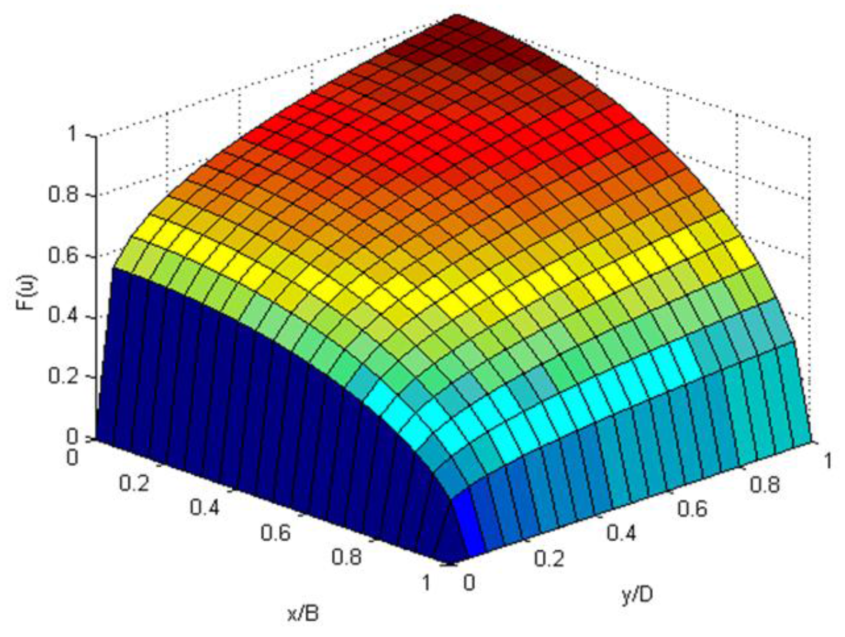
Different types of hypotheses have been formulated when applying entropy theory to derive relationships for design variables. Examples of a linear hypothesis include velocity distribution as a function of flow depth, wind velocity as a function of height, sediment concentration profile along the flow depth, rating curve and groundwater discharge along the horizontal direction of flow. It is noted that the CDF should have a one-to-one relation with the design variable (i.e., random variable) of interest and its value should only be between 0 and 1; 0 for the minimum value of the random variable and 1 for the maximum value. For deriving a two-dimensional velocity (u) distribution, Cui and Singh [77] hypothesized a general form of the CDF as:
in which y is the vertical dimension, x is the transverse direction, a and b are shape parameters and B and D act as scale parameters or normalizing quantities. The CDF given by Equation (54) has a one-to-one relationship with the velocity value u; in other words, the CDF is unique on each isovel I(u) and has a value of 0 at I(0) and 1 at I(umax). Also, CDF is 0 at x = B or y = 0 and is 1 at x = 0 and y = D (Figure 3). It is continuous and differentiable in both x and y.
The two-dimensional (2-D) velocity distribution can also be expressed by transforming the Cartesian coordinates [vertical (y) and transverse (x)] into curvilinear s-r coordinate system in which r has a unique, one-to-one relation with a value of velocity and s (coordinate) curves are their orthogonal trajectories [56]. Then, the CDF of velocity in a channel cross section can be expressed as:
where r is a coordinate between r0 and rmax and corresponds to y.
For the one-dimensional (1-D) form of Equation (54) with b = 0, it is seen from Equation (54) that the CDF will remain between 0 and 1 when 0 ≤ x ≤ B and 0 ≤ y ≤ D. Thus, the CDF for 1-D velocity distribution can be simplified as:
This equation implies that the shape parameter a is critical. If a = 1, then
In cases where the design variable is maximum at y = 0 and minimum at maximum y (i.e., y = D), as is the case for suspended sediment concentration, it is distributed from a maximum value at the channel bed and decreases towards the water surface. Hence, the CDF should be assumed in a way so that it is 1 at the channel bed (y = 0) and 0 at the water surface (y = D). The CDF of sediment concentration can then be expressed as:
It is seen from Equation (58) that F(c) will be between 0 and 1 if 0 ≤ y ≤ D.
6.2. One-Dimensional Velocity Distribution
Velocity distribution is needed for determining flow discharge, scour around bridge piers, erosion and sediment transport, pollutant transport, energy and momentum distribution coefficients, hydraulic geometry, watershed runoff and river behavior. Velocity distributions have been derived using experimental, hydrodynamic, or entropy methods. Shannon entropy has been applied to derive one- and two-dimensional velocity distributions [26]. Singh and Luo [11,78] and Luo and Singh [12] employed Tsallis entropy to derive the 1-D velocity distribution. The Tsallis entropy-based velocity distribution has been shown to have an advantage over the Shannon entropy-based distribution. However, in these entropy-based velocity distributions, the CDF has been assumed to be linear, meaning the velocity is equally likely along the vertical from the channel bed to the water surface. This assumption is fundamental to the derivation of velocity distributions but has not been adequately scrutinized. Further, this assumption is weak and may partly explain the reason why these velocity distributions do not accurately describe the velocity near the channel bed.
For deriving 1-D velocity distribution, the constraint equation is derived using the continuity equation such that g1(u) = u and limits of integration are 0 and uD (maximum velocity at the surface or flow depth D). The entropy theory then yields the probability density function of velocity u:
where .
Following Cui and Singh [77], the CDF of u can be hypothesized as Equation (56). Then, a general velocity distribution based on the Tsallis entropy theory [14] is obtained as:
Equation (60) can be simplified by defining a dimensionless parameter G as:
Parameter G can be regarded as an index of the velocity distribution uniformity. Equation (60) can be cast as:
Equation (62) shows that for a given m value, the velocity distribution can be obtained with only two parameters: a and G. A bigger G value tends to slow the growth of the velocity from the channel bed to the water surface, while the parameter a has an opposite effect. A lower value of G tends to linearize the velocity distribution and a higher value non-linearize. The opposite is the case for exponent a. The velocity distribution is more sensitive to a than to G.
6.3. Two-Dimensional Velocity Distribution
For two-dimensional (2-D) velocity distribution, Chiu [56] proposed a transformation that converts the Cartesian coordinates [vertical (y) and transverse (z)] into curvilinear s-r coordinate system, in which r has a unique, one-to-one relation with a value of velocity and s (coordinate) curves are orthogonal trajectories to r. Following the coordinate system of Chiu [56], Luo and Singh [12] employed the Tsallis entropy. Then, expressing the CDF of velocity in a channel cross section by Equation (57), the velocity distribution becomes
Defining entropy parameter , the dimensionless velocity distribution can be expressed as:
The Tsallis entropy-based approach of Luo and Singh [12] was either superior or comparable to Chiu’s distribution for the data sets used therein for testing. However, due to the complexity of the coordinate system and a large number of parameters used, the application of these methods may be limited. Later, using normal x-y coordinate system, Cui and Singh [13] obtained the 2-D velocity distribution equation as:
where the CDF, F(u), is defined as Equation (54). As defined in the case of one-dimensional velocity distribution, the dimensionless entropy parameter G is also used here as:
Parameter G is found to be related to the ratio of mean and maximum velocity and a quadratic relation is obtained by computing from observed mean and maximum velocity values as [13]:
Now, with the use of Equation (67), the general velocity distribution Equation (65) can be cast as:
Equation (68) is the general 2-D velocity distribution equation in terms of parameter G and maximum velocity.
6.4. Suspended Sediment Concentration
The sediment concentration distribution can also be derived using Tsallis entropy. For deriving the one-dimensional sediment concentration distribution, the constraint equation is derived using the mean concentration, such that g1(c) = c and limits of integration are a = c0 (maximum concentration at the bed surface or flow depth D = 0) and b = 0 at the water surface, as [16]:
where . Equation (69) is the least-biased entropy-based probability density function of sediment concentration, which is fundamental to determining the sediment concentration distribution. The dimensionless sediment concentration can then be obtained as:
where N is a dimensionless parameter as a function of maximum concentration and the Lagrange multipliers expressed as:
By plotting the empirical observations of the mean over the maximum concentration values and corresponding N values, the implicit function can be regressed as a quadratic polynomial as:
with a coefficient of determination as 0.99. Thus, N can be used for deriving sediment concentration distribution instead of solving nonlinear equations for λ1 and .
6.5. Sediment Discharge
The suspended sediment discharge can be computed simultaneously by integrating sediment concentration and velocity over the cross-section where the velocity distribution and sediment concentration can be obtained empirically as well as using the Tsallis entropy theory. That is, suspended sediment discharge can be derived using different combinations of entropy-based and empirical methods for velocity and sediment concentration distributions. Thus, the suspended sediment discharge can be computed with the use of entropy in three ways: (1) velocity distribution by a standard formula and concentration distribution by an entropy-based equation; (2) velocity distribution by an entropy-based equation and concentration distribution by a standard formula; and (3) velocity distribution and concentration distribution both by entropy-based equations. In the discussion that follows, only the combination where both are derived using Tsallis entropy is considered.
The Tsallis entropy-based velocity distribution [13], given by Equation (68) and sediment concentration [16], given by Equation (70), are integrated from bottom of the channel to the water surface to obtain the suspended sediment discharge, as:
To get an explicit solution of Equation (73) is difficult; however, it can be simplified with the use of mean values. The first term in the integration can be replaced by mean sediment concentration and the second term can be replaced by mean velocity, such that Equation (73) reduces to
which provides a simple method to compute sediment discharge. Entropy parameters G and N are fixed for each channel cross-section [17]. Thus, once the entropy parameters have been obtained for some known cross-section, with observed maximum velocity and sediment concentration, the sediment discharge can be obtained with ease.
6.6. Flow-Duration Curve
The flow-duration curve (FDC) is used for predicting the distribution of future flows, forecasting of future recurrence frequencies, determining low-flow thresholds for defining droughts, generating hydropower, constructing load-duration curves, determining power-duration curves and comparing watersheds. For deriving an FDC, it is assumed that temporally-averaged discharge Q is a random variable, varying from a minimum value Qmin to a maximum value Qmax, with a probability density function (PDF) denoted as f(Q). The time interval for which the discharge is averaged depends on the purpose of constructing an FDC but it is often taken as one day. Considering g1(x) = mean Q = Qmean, the PDF of Q can be derived as [79]:
It is interesting to note that at Q = 0, f(Q) becomes Similar to velocity distribution, a dimensionless parameter M can be defined as:
It was found [79] that M is linearly related to the ratio between the mean flow and the maximum flow, which, using regression, can be written as:
with the squared correlation coefficient of 0.9972. The FDC can be expressed as:
7. Conclusions
A survey of the literature shows that the Tsallis entropy theory has great potential to address a wide range of problems in water engineering and in many other fields, as reviewed in this paper; see also [80,81,82,83,84,85] for some more recent studies. As generalization of the Shannon entropy, the Tsallis entropy can be applied in generalized equilibrium and statics in physics. The advantage of using the theory is that it can combine statistical information with physical laws, permits deriving physical relations as functions of time or space and derives probability distributions in terms of the specified constraints. However, analysis using the Tsallis entropy theory becomes complicated when one or two constraints are involved and it is more difficult to obtain the analytical expressions. Besides, the m-statistic must be carefully chosen when applying the Tsallis entropy, since it sometimes involves complex operations. Although entropy is a thermodynamic quantity, development of the thermodynamic basis of entropy-based relations has not been accomplished yet. Until now, the Tsallis entropy has been applied to determine frequency distributions, network evaluation, hydraulic geometry, evaporation, velocity distribution, sediment concentration distribution, flow duration curves and several other problems, as reviewed above. The outcomes are certainly encouraging. Until now, as we have reviewed in this paper, the Tsallis entropy theory has been applied in water engineering particularly with the principle of maximum entropy (POME). There is, however, also potential to combine the Tsallis entropy with the minimum relative (cross) entropy, for the condition that prior assumptions can be made. There is no question that the Tsallis entropy theory has a much greater potential to study a wide spectrum of problems in water engineering. It is hoped that this review will stimulate further interest in this fascinating field.
Acknowledgments
Bellie Sivakumar acknowledges the financial support from the Australian Research Council (ARC) through the Future Fellowship grant (FT110100328). Huijuan Cui acknowledges the financial support from Key Research Program of the Chinese Academy of Sciences (ZDRW-ZS-2016-6-4).
Author Contributions
All three authors substantially contributed to the article. Vijay P. Singh conceived the ideas for this review article; Vijay P. Singh, Bellie Sivakumar and Huijuan Cui had detailed discussions about the contents, structure and organization of the manuscript; Vijay P. Singh prepared the initial draft; Bellie Sivakumar and Huijuan Cui contributed to modifications and improvements; Vijay P. Singh, Bellie Sivakumar and Huijuan Cui contributed to the responses to the review comments and manuscript revision.
Conflicts of Interest
The authors declare no conflict of interest.
Notation
| B | channel width |
| c | sediment concentration |
| Cr | constraint |
| D | water depth |
| E | evaporation |
| f(x) | probability density function |
| G | ground heat flux |
| H | entropy |
| ΔI(xi) | gain in information |
| k = (1 − m)/m | |
| m | Tsallis entropy index |
| n | Manning’s n |
| N | natural number representative |
| pi | probability |
| Q | flow |
| qs | sediment discharge |
| R | net radiative |
| Sj | entropic measure of redundancy |
| u | velocity |
| x | transverse direction |
| y | vertical dimension |
| σ2 | variance |
| λi | Langrange multiplier |
| μ1 | first moment |
| μ2 | second moment |
| w | surface soil moisture |
References
- Singh, V.P. Hydrologic Systems: Vol. 1. Rainfall-Runoff Modeling; Prentice Hall: Englewood Cliffs, NJ, USA, 1988. [Google Scholar]
- Singh, V.P. Hydrologic Systems: Vol. 2. Watershed Modeling; Prentice Hall: Englewood Cliffs, NJ, USA, 1989. [Google Scholar]
- Singh, V.P. (Ed.) Computer Models of Watershed Hydrology; Water Resources Publications: Highland Ranch, CO, USA, 1995. [Google Scholar]
- Salas, J.D.; Delleur, J.W.; Yevjevich, V.; Lane, W.L. Applied Modeling of Hydrologic Time Series; Water Resources Publications: Littleton, CO, USA, 1995. [Google Scholar]
- Beven, K.J. Rainfall-Runff Modelling: The Primer; Wiley: Chichester, UK, 2001. [Google Scholar]
- Sivakumar, B.; Berndtsson, R. Advances in Data-Based Approaches for Hydrologic Modeling and Forecasting; World Scientific Publishing Company: Singapore, 2010. [Google Scholar]
- Singh, V.P. Handbook of Applied Hydrology, 2nd ed.; McGraw-Hill Education: New York, NY, USA, 2017. [Google Scholar]
- Singh, V.P. Kinematic Wave Modeling in Water Resources: Surface Water Hydrology; John Wiley & Sons: New York, NY, USA, 1995. [Google Scholar]
- Singh, V.P. Kinematic Wave Modeling in Water Resources: Environmental Hydrology; John Wiley & Sons: New York, NY, USA, 1996. [Google Scholar]
- Harmancioglu, N.B.; Fistikoglu, O.; Ozkul, S.D.; Singh, V.P.; Alpaslan, M.N. Water Quality Monitoring Network Design; Kluwer Academic Publishers: Boston, MA, USA, 1999; p. 299. [Google Scholar]
- Singh, V.P.; Luo, H. Entropy theory for distribution of one-dimensional velocity in open channels. J. Hydrol. Eng. 2011, 16, 725–735. [Google Scholar] [CrossRef]
- Luo, H.; Singh, V.P. Entropy theory for two-dimensional velocity distribution. J. Hydrol. Eng. 2011, 16, 303–315. [Google Scholar] [CrossRef]
- Cui, H.; Singh, V.P. Two-dimensional velocity distribution in open channels using the Tsallis entropy. J. Hydrol. Eng. 2013, 18, 331–339. [Google Scholar] [CrossRef]
- Cui, H.; Singh, V.P. One-dimensional velocity distribution in open channels using Tsallis entropy. J. Hydrol. Eng. 2014, 19, 290–298. [Google Scholar] [CrossRef]
- Simons, D.B.; Senturk, F. Sediment Transport Technology; Water Resources Publications: Highland Ranch, CO, USA, 1976. [Google Scholar]
- Cui, H.; Singh, V.P. Suspended sediment concentration in open channels using Tsallis entropy. J. Hydrol. Eng. 2014, 19, 966–977. [Google Scholar] [CrossRef]
- Cui, H.; Singh, V.P. Computation of suspended sediment discharge in open channels by combining Tsallis entropy-based methods and empirical formulas. J. Hydrol. Eng. 2014, 19, 18–25. [Google Scholar] [CrossRef]
- Singh, V.P. On the theories of hydraulic geometry. Int. J. Sediment Res. 2003, 18, 196–218. [Google Scholar]
- Singh, V.P.; Yang, C.T.; Deng, Z.Q. Downstream hydraulic geometry relations: 1. Theoretical development. Water Resour. Res. 2003, 39, 1337. [Google Scholar] [CrossRef]
- Singh, V.P.; Yang, C.T.; Deng, Z.Q. Downstream hydraulic geometry relations: 2. Calibration and testing. Water Resour. Res. 2003, 39, 1338. [Google Scholar] [CrossRef]
- Singh, V.P.; Zhang, L. At-a-station hydraulic geometry: I. Theoretical development. Hydrol. Process. 2008, 22, 189–215. [Google Scholar] [CrossRef]
- Singh, V.P.; Zhang, L. At-a-station hydraulic geometry: II. Calibration and testing. Hydrol. Process. 2008, 22, 216–228. [Google Scholar] [CrossRef]
- Singh, V.P.; Oh, J. A Tsallis entropy-based redundancy measure for water distribution network. Physica A 2014, 421, 360–376. [Google Scholar] [CrossRef]
- Singh, V.P. Entropy Theory and Its Application in Environmental and Water Engineering; John Wiley & Sons: Sussex, UK, 2013. [Google Scholar]
- Singh, V.P. Entropy Theory in Hydraulic Engineering: An Introduction; ASCE Press: Reston, VA, USA, 2014. [Google Scholar]
- Singh, V.P. Entropy Theory in Hydrologic Science and Engineering; McGraw-Hill Education: New York, NY, USA, 2015. [Google Scholar]
- Koutsoyiannis, D. Physics of uncertainty, the Gibbs paradox and indistinguishable particles. Stud. Hist. Philos. Mod. Phys. 2013, 44, 480–489. [Google Scholar] [CrossRef]
- Papalexiou, S.M.; Koutsoyiannis, D. Entropy based derivation of probability distributions: A case study to daily rainfall. Adv. Water Resour. 2012, 45, 51–57. [Google Scholar] [CrossRef]
- Shannon, C.E. The mathematical theory of communications, I and II. Bell Syst. Tech. J. 1948, 27, 379–423. [Google Scholar] [CrossRef]
- Tsallis, C. Possible generalization of Boltzmann-Gibbs statistics. J. Stat. Phys. 1988, 52, 479–487. [Google Scholar] [CrossRef]
- Singh, V.P. The use of entropy in hydrology and water resources. Hydrol. Process. 1997, 11, 587–626. [Google Scholar] [CrossRef]
- Singh, V.P. Hydrologic synthesis using entropy theory: Review. J. Hydrol. Eng. 2011, 16, 421–433. [Google Scholar] [CrossRef]
- Singh, V.P. Introduction to Tsallis Entropy Theory in Water Engineering; CRC Press/Taylor and Francis: Boca Raton, FL, USA, 2016. [Google Scholar]
- Tsallis, C. Entropic nonextensivity: A possible measure of complexity. Chaos Solitons Fractals 2002, 12, 371–391. [Google Scholar] [CrossRef]
- Tsallis, C. On the fractal dimension of orbits compatible with Tsallis statistics. Phys. Rev. E 1998, 58, 1442–1445. [Google Scholar] [CrossRef]
- Niven, R.K. The constrained entropy and cross-entropy functions. Physica A 2004, 334, 444–458. [Google Scholar] [CrossRef]
- Koutsoyiannis, D. Uncertainty, entropy, scaling and hydrological stochastics. 1. Marginal distributional properties of hydrological processes and state scaling. Hydrol. Sci. J. 2005, 50, 381–404. [Google Scholar] [CrossRef]
- Koutsoyiannis, D. Uncertainty, entropy, scaling and hydrological stochastics. 2. Time dependence of hydrological processes and time scaling. Hydrol. Sci. J. 2005, 50, 405–426. [Google Scholar] [CrossRef]
- Koutsoyiannis, D. A toy model of climatic variability with scaling behavior. J. Hydrol. 2005, 322, 25–48. [Google Scholar] [CrossRef]
- Tsallis, C. Nonextensive statistical mechanics: Construction and physical interpretation. In Nonextensive Entropy-Interdisciplinary Applications; Gell-Mann, M., Tsallis, C., Eds.; Oxford University Press: New York, NY, USA, 2004; pp. 1–52. [Google Scholar]
- Tsallis, C. Nonextensive statistical mechanics and thermodynamics: Historical background and present status. In Nonextensive Statistical Mechanics and Its Applications; Abe, S., Okamoto, Y., Eds.; Series Lecture Notes in Physics; Springer: Berlin, Germany, 2001. [Google Scholar]
- Jaynes, E.T. Information theory and statistical mechanics, I. Phys. Rev. 1957, 106, 620–630. [Google Scholar] [CrossRef]
- Jaynes, E.T. Information theory and statistical mechanics, II. Phys. Rev. 1957, 108, 171–190. [Google Scholar] [CrossRef]
- Kullback, S.; Leibler, R.A. On information and sufficiency. Ann. Math. Stat. 1951, 22, 79–86. [Google Scholar] [CrossRef]
- Lombardo, F.; Volpi, E.; Koutsoyiannis, D.; Papalexiou, S.M. Just two moments! A cautionary note against use of high-order moments in multifractal models in hydrology. Hydrol. Earth Syst. Sci. 2014, 18, 243–255. [Google Scholar] [CrossRef]
- Krstanovic, P.F.; Singh, V.P. A univariate model for longterm streamflow forecasting: I. Development. Stoch. Hydrol. Hydraul. 1991, 5, 173–188. [Google Scholar] [CrossRef]
- Krstanovic, P.F.; Singh, V.P. A univariate model for longterm streamflow forecasting: II. Application. Stoch. Hydrol. Hydraul. 1991, 5, 189–205. [Google Scholar] [CrossRef]
- Krstanovic, P.F.; Singh, V.P. A real-time flood forecasting model based on maximum entropy spectral analysis: I. Development. Water Resour. Manag. 1993, 7, 109–129. [Google Scholar] [CrossRef]
- Krstanovic, P.F.; Singh, V.P. A real-time flood forecasting model based on maximum entropy spectral analysis: II. Application. Water Resour. Manag. 1993, 7, 131–151. [Google Scholar] [CrossRef]
- Krasovskaia, I. Entropy-based grouping of river flow regimes. J. Hydrol. 1997, 202, 173–191. [Google Scholar] [CrossRef]
- Krasovskaia, I.; Gottschalk, L. Stability of river flow regimes. Nordic Hydrol. 1992, 23, 137–154. [Google Scholar]
- Singh, V.P. Entropy-Based Parameter Estimation in Hydrology; Kluwer Academic Publishers: Boston, MA, USA, 1998; p. 365. [Google Scholar]
- Wang, J.; Bras, R.L. A model of evapotranspiration based on the theory of maximum entropy production. Water Resour. Res. 2011, 47, W03521. [Google Scholar] [CrossRef]
- Yang, C.T. Unit stream power and sediment transport. J. Hydraul. Div. ASCE 1972, 98, 1805–1826. [Google Scholar]
- Fiorentino, M.; Claps, P.; Singh, V.P. An entropy-based morphological analysis of river-basin networks. Water Resour. Res. 1993, 29, 1215–1224. [Google Scholar] [CrossRef]
- Chiu, C.L. Entropy and 2-D velocity distribution in open channels. J. Hydraul. Eng. ASCE 1988, 114, 738–756. [Google Scholar] [CrossRef]
- Cao, S.; Knight, D.W. Design of threshold channels. Hydra 2000. In Proceedings of the 26th IAHR Congress, London, UK, 11–15 September 1995. [Google Scholar]
- Cao, S.; Knight, D.W. New Concept of hydraulic geometry of threshold channels. In Proceedings of the 2nd Symposium on the Basic Theory of Sedimentation, Beijing, China, 30 October–2 November 1995. [Google Scholar]
- Cao, S.; Knight, D.W. Entropy-based approach of threshold alluvial channels. J. Hydraul. Res. 1997, 35, 505–524. [Google Scholar] [CrossRef]
- Singh, V.P. Entropy theory for movement of moisture in soils. Water Resour. Res. 2010, 46, 1–12. [Google Scholar] [CrossRef]
- Singh, V.P. Tsallis entropy theory for derivation of infiltration equations. Trans. ASABE 2010, 53, 447–463. [Google Scholar] [CrossRef]
- Evans, M.; Hastings, N.; Peacock, B. Statistical Distributions; John Wiley & Sons: New York, NY, USA, 2000. [Google Scholar]
- Krstanovic, P.F.; Singh, V.P. Evaluation of rainfall networks using entropy: 1. Theoretical development. Water Resour. Manag. 1992, 6, 279–293. [Google Scholar] [CrossRef]
- Krstanovic, P.F.; Singh, V.P. Evaluation of rainfall networks using entropy: 2. Application. Water Resour. Manag. 1992, 6, 295–314. [Google Scholar] [CrossRef]
- Yang, Y.; Burn, D.H. An entropy approach to data collection network design. J. Hydrol. 1994, 157, 307–324. [Google Scholar] [CrossRef]
- Mogheir, Y.; Singh, V.P. Application of information theory to groundwater quality monitoring networks. Water Resour. Manag. 2002, 16, 37–49. [Google Scholar] [CrossRef]
- Perelman, L.; Ostfeld, A.; Salomons, E. Cross entropy multiobjective optimization for water distribution systems design. Water Resour. Res. 2008, 44, W09413. [Google Scholar] [CrossRef]
- Goulter, I.C. Current and future use of systems analysis in water distribution network design. Civ. Eng. Syst. 1987, 4, 175–184. [Google Scholar] [CrossRef]
- Goulter, I.C. Assessing the reliability of water distribution networks using entropy based measures of network redundancy. In Entropy and Energy Dissipation in Water Resources; Singh, V.P., Fiorentino, M., Eds.; Kluwer Academic Publishers: Dordrecht, The Netherlands, 1992; pp. 217–238. [Google Scholar]
- Walters, G. Optimal design of pipe networks: A review. In Proceedings of the 1st International Conference Computational Water Resources, Rabat, Morocco, 14–18 March 1988; Computational Mechanics Publications: Southampton, UK, 1988; pp. 21–31. [Google Scholar]
- Leopold, L.B.; Maddock, T.J. Hydraulic Geometry of Stream Channels and Some Physiographic Implications; US Government Printing Office: Washington, DC, USA, 1953; p. 55.
- Langbein, W.B. Geometry of river channels. J. Hydraul. Div. ASCE 1964, 90, 301–311. [Google Scholar]
- Yang, C.T.; Song, C.C.S.; Woldenberg, M.J. Hydraulic geometry and minimum rate of energy dissipation. Water Resour. Res. 1981, 17, 1014–1018. [Google Scholar] [CrossRef]
- Wolman, M.G. The Natural Channel of Brandywine Creek, Pennsylvania; US Government Printing Office: Washington, DC, USA, 1955.
- Williams, G.P. Hydraulic Geometry of River Cross-Sections-Theory of Minimum Variance; US Government Printing Office: Washington, DC, USA, 1978.
- Wang, J.; Salvucci, G.D.; Bras, R.L. A extremum principle of evaporation. Water Resour. Res. 2004, 40, W09303. [Google Scholar] [CrossRef]
- Cui, H.; Singh, V.P. ON the cumulative distribution function for entropy-based hydrologic modeling. Trans. ASABE 2012, 55, 429–438. [Google Scholar] [CrossRef]
- Singh, V.P.; Luo, H. Derivation of velocity distribution using entropy. In Proceedings of the IAHR Congress, Vancouver, BC, Canada, 9–14 August 2009; pp. 31–38. [Google Scholar]
- Singh, V.P.; Byrd, A.; Cui, H. Flow duration curve using entropy theory. J. Hydrol. Eng. 2014, 19, 1340–1348. [Google Scholar] [CrossRef]
- Weijs, S.V.; van de Giesen, N.; Parlange, M.B. HydroZIP: How hydrological knowledge can be used to improve compression of hydrological data. Entropy 2013, 15, 1289–1310. [Google Scholar] [CrossRef] [Green Version]
- Chen, J.; Li, G. Tsallis wavelet entropy and its application in power signal analysis. Entropy 2014, 16, 3009–3025. [Google Scholar] [CrossRef]
- Furuichi, S.; Mitroi-Symeonidis, F.-C.; Symeonidis, E. On some properties of Tsallis hypoentropies and hypodivergences. Entropy 2014, 16, 5377–5399. [Google Scholar] [CrossRef]
- Lenzi, E.K.; da Silva, L.R.; Lenzi, M.K.; dos Santos, M.A.F.; Ribeiro, H.V.; Evangelista, L.R. Intermittent motion, nonlinear diffusion equation and Tsallis formalism. Entropy 2017, 19, 42. [Google Scholar] [CrossRef]
- Evren, A.; Ustaoğlu, E. Measures of qualitative variation in the case of maximum entropy. Entropy 2017, 19, 204. [Google Scholar] [CrossRef]
- Kalogeropoulos, N. The Legendre transform in non-additive thermodynamics and complexity. Entropy 2017, 19, 298. [Google Scholar] [CrossRef]
Figure 1.
Gain function for m = −1, 0, 1 and 2.

Figure 2.
Plot of H for m = −1, –0.5, 0, 0.5, 1 and 2.
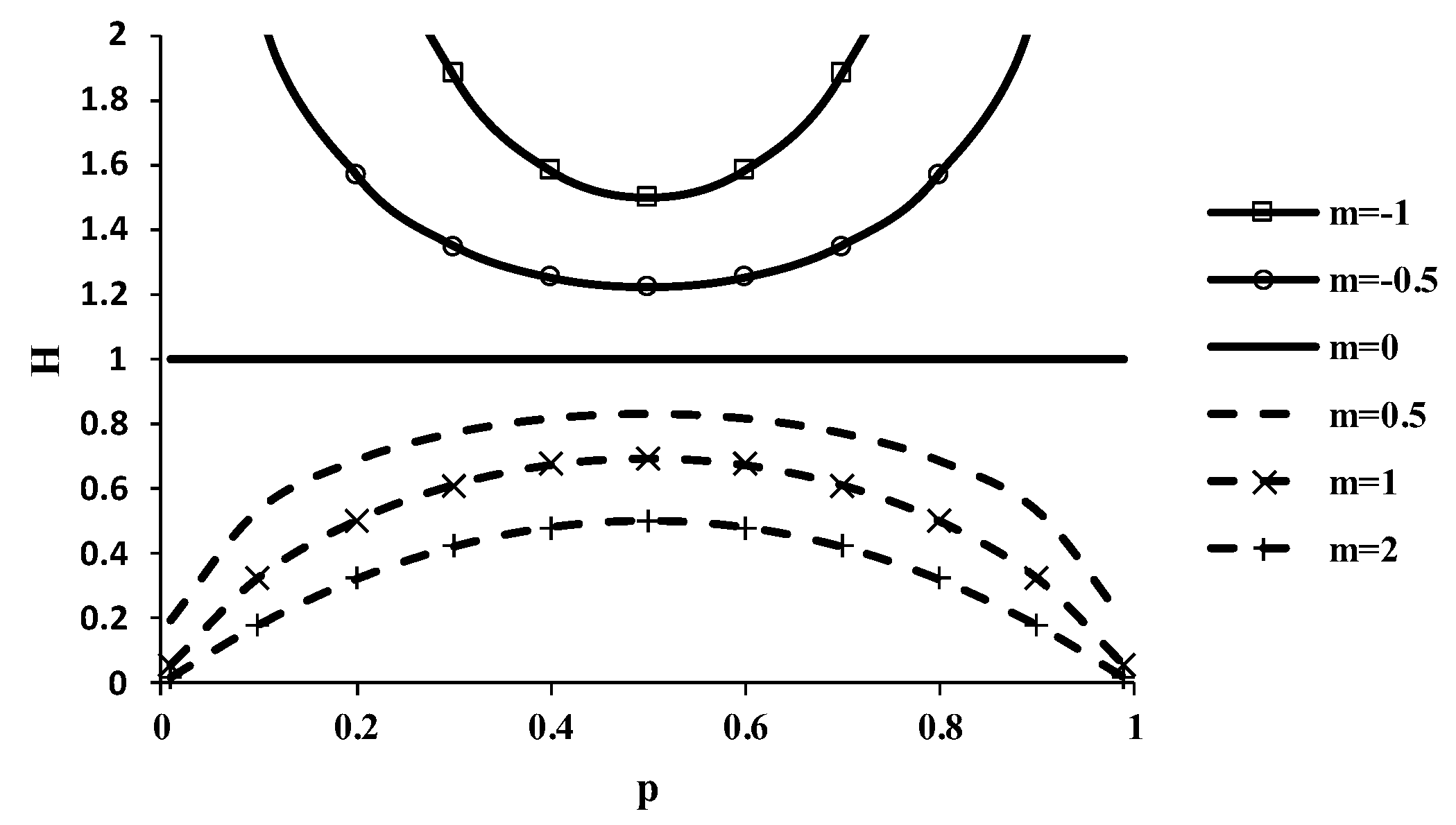
Figure 3.
CDF of 2-D velocity distribution with a = 0.5, b = 0.2 in the idealized cross-section.

© 2017 by the authors. Licensee MDPI, Basel, Switzerland. This article is an open access article distributed under the terms and conditions of the Creative Commons Attribution (CC BY) license (http://creativecommons.org/licenses/by/4.0/).
Share and Cite
MDPI and ACS Style
Singh, V.P.; Sivakumar, B.; Cui, H. Tsallis Entropy Theory for Modeling in Water Engineering: A Review. Entropy 2017, 19, 641. https://doi.org/10.3390/e19120641
AMA Style
Singh VP, Sivakumar B, Cui H. Tsallis Entropy Theory for Modeling in Water Engineering: A Review. Entropy. 2017; 19(12):641. https://doi.org/10.3390/e19120641
Chicago/Turabian StyleSingh, Vijay P., Bellie Sivakumar, and Huijuan Cui. 2017. "Tsallis Entropy Theory for Modeling in Water Engineering: A Review" Entropy 19, no. 12: 641. https://doi.org/10.3390/e19120641
Note that from the first issue of 2016, this journal uses article numbers instead of page numbers. See further details here.