Information Theory to Probe Intrapartum Fetal Heart Rate Dynamics
by

Carlos Granero-Belinchon
1, 
Stéphane G. Roux
1,
Patrice Abry
1,
Muriel Doret
2 and
Nicolas B. Garnier
1,* 1
Laboratoire de Physique, CNRS, Universitè Claude Bernard Lyon 1, ENS de Lyon, Universitè de Lyon, F-69342 Lyon, France
2
Hôpital Femme Mère Enfant, Universitè Lyon I, F-69677 Bron, France
*
Author to whom correspondence should be addressed.
Entropy 2017, 19(12), 640; https://doi.org/10.3390/e19120640
Submission received: 18 October 2017
/
Revised: 21 November 2017
/
Accepted: 21 November 2017
/
Published: 25 November 2017
(This article belongs to the Special Issue Entropy and Cardiac Physics II)
Abstract
:Intrapartum fetal heart rate (FHR) monitoring constitutes a reference tool in clinical practice to assess the baby’s health status and to detect fetal acidosis. It is usually analyzed by visual inspection grounded on FIGO criteria. Characterization of intrapartum fetal heart rate temporal dynamics remains a challenging task and continuously receives academic research efforts. Complexity measures, often implemented with tools referred to as approximate entropy (ApEn) or sample entropy (SampEn), have regularly been reported as significant features for intrapartum FHR analysis. We explore how information theory, and especially auto-mutual information (AMI), is connected to ApEn and SampEn and can be used to probe FHR dynamics. Applied to a large (1404 subjects) and documented database of FHR data, collected in a French academic hospital, it is shown that (i) auto-mutual information outperforms ApEn and SampEn for acidosis detection in the first stage of labor and continues to yield the best performance in the second stage; (ii) Shannon entropy increases as labor progresses and is always much larger in the second stage; (iii) babies suffering from fetal acidosis additionally show more structured temporal dynamics than healthy ones and that this progressive structuration can be used for early acidosis detection.
1. Introduction
Intrapartum fetal heart rate monitoring:
Because it is likely to provide obstetricians with significant information related to the health status of the fetus during delivery, intrapartum fetal heart rate (FHR) monitoring is a routine procedure in hospitals. Notably, it is expected to permit detection of fetal acidosis, which may induce severe consequences for both the baby and the mother and thus requires a timely and relevant decision for rapid intervention and operative delivery [1]. In daily clinical practice, FHR is mostly inspected visually, through training by clinical guidelines formalized by the International Federation of Gynecology and Obstetrics (FIGO) [2,3]. However, it has been well documented that such visual inspection is prone to severe inter-individual variability and even shows a substantial intra-individual variability [4]. This reflects both that FHR temporal dynamics are complex and hard to assess and that FIGO criteria lead to a demanding evaluation, as they mix several aspects of FHR dynamics (baseline drift, decelerations, accelerations, long- and short-term variabilities). Difficulties in performing objective assessment of these criteria has led to a substantial number of unnecessary Caesarean sections [5]. This has triggered a large amount of research world wide aiming both to compute in a reproducible and objective way the FIGO criteria [2] and to devise new signal processing-inspired features to characterize FHR temporal dynamics (cf. [6,7] for reviews).
Related works:
After the seminal contribution in the analysis of heart rate variability (HRV) in adults [8], spectrum estimation has been amongst the first signal processing tools that has been considered for computerized analysis of FHR, either constructed on models driven by characteristic time scales [9,10,11] or the scale-free paradigm [12,13,14]. Further, aiming to explore temporal dynamics beyond the mere temporal correlations, several variations of nonlinear analysis have been envisaged both for antepartum and intrapartum FHR [15], based, e.g., on multifractal analysis [13], scattering transforms [16], phase-driven synchronous pattern averages [17] or complexity and entropy measures [18,19,20]. Interested readers are referred to e.g., [6,7] for overviews. There has also been several attempts to combine features different in nature by doing multivariate classification using supervised machine learning strategies (cf. e.g., [6,21,22,23,24]).
Measures from complexity theory or information theory remain however amongst the most used tools to construct HRV characterization. They are defined independently from (deterministic) dynamical systems or from (random) stochastic process frameworks. The former led to standard references, both for adult and for antepartum and intrapartum fetal heart rate analysis: approximate entropy (ApEn) [18,25] and sample entropy (SampEn) [26], which can be regarded as practical approximations to Kolmogorov–Sinai or Eckmann–Ruelle complexity measures. The stochastic process framework leads to the definitions of Shannon and Rényi entropies and entropy rates. Both worlds are connected by several relations, cf., e.g., [27,28] for reviews. Implementations of ApEn and SampEn rely on the correlation integral-based algorithm (CI) [18,29], while that of Shannon entropy rates may instead benefit from the k-nearest neighbor (k-NN) algorithm [30], which brings robustness and improved performance to entropy estimation [31,32,33].
Labor stages:
Automated FHR analysis is complicated by the existence of two distinct stages during labor. The dilatation stage (Stage 1) consists of progressive cervical dilatation and regular contractions. The active pushing stage (Stage 2) is characterized by a fully-dilated cervix and expulsive contractions. The most common approaches in FHR analysis consist of not distinguishing stages and performing a global analysis [23,34] or of focusing on Stage 1 only, as it is better documented and usually shows data with better quality, cf., e.g., [24,35]. Whether or not temporal dynamics associated with each stage are different has not been intensively explored yet (see a contrario [36,37]). However, recently, some contributions have started to conduct systematic comparisons [38,39].
Goals, contributions and outline:
The present contribution remains in the category of works aiming to design new efficient features for FHR, here based on advanced information theoretic concepts. These new tools are applied to a high quality, large (1404 subjects) and documented FHR database collected across years in an academic hospital in France and described in Section 2. The database is split into two datasets associated each with one stage of labor, which enables us first to assess and compare acidosis detection performance achieved by the proposed features independently at each stage and second to address differences in FHR temporal dynamics between the two stages. Reexamining formally the definitions of entropy rates in information theory, Section 3.1 first establishes that they can be split into two components: Shannon entropy, which quantifies data static properties, and auto-mutual information (AMI), which characterizes temporal dynamics in data, combining both linear and nonlinear (or higher order) statistics. ApEn and SampEn, defined from complexity theory, are then explicitly related to entropy rates and, hence, to AMI (cf. Section 3.3). Estimation procedures for Shannon entropy, entropy rate and AMI, based on k-nearest neighbor (k-NN) algorithms [30], are compared to those of ApEn and SampEn, constructed on correlation integral algorithms [18,29,40]. Acidosis detection performances are reported in Section 4.1. Results are discussed in terms of quality versus analysis window size, k-NN or correlation integral-based procedures and differences between Stages 1 and 2. Further, a longitudinal study consisting of sliding analysis in overlapping windows across the delivery process permits showing that processes characterizing Stages 1 and 2 are different (Section 4.4).
2. Datasets: Intrapartum Fetal Heart Rate Times Series and Labor Stages
Data collection:
Intrapartum fetal heart rate data were collected at the academic Femme-Mère-Enfant hospital, in Lyon, France, during daily routine monitoring across the years 2000 to 2010. They were recorded using STAN S21 or S31 devices with internal scalp electrodes at 12-bit resolution, 500-Hz sampling rate (STAN, Neoventa Medical, Sweden). Clinical information was provided by the obstetrician in charge, reporting delivery conditions, as well as the health status of the baby, notably the umbilical artery pH after delivery and the decision for intervention due to suspected acidosis [41].
Datasets:
For the present study, subjects were included using criteria detailed in [24,41], leading to a total of 1404 tracings, lasting from 30 min to several hours. These criteria essentially aim to reject subjects with too low quality recording (e.g., too many missing data, too large gaps, too short recordings, etc.). As a result, for subjects in the database, the average fraction of data missing in the last 20 min before delivery is less than 5%. The first goal of the present work is to assess the relevance of new information theoretic measures; their robustness to poor quality data is postponed for future work.
The measurement of pH, performed by blood test immediately after delivery, is systematically documented and used as the ground-truth: When pH , the newborn is considered has having suffered from acidosis and is referred to as acidotic (A, pH ). Conversely, when pH , the newborn is considered not having suffered from acidosis during delivery and is termed normal (N, pH ). In order to have a meaningful pH indication, we retain only subjects for which the time between end of recording and birth is lower than or equal to 10 min.
Following the discussion above on labor stages, subjects are split into two different datasets. Dataset I consists of subjects for which delivery took place after a short Stage 2 (less than 15 min) or during Stage 1 (Stage 2 was absent). It contains 913 normal and 26 acidotic subjects. Dataset II gathers FHR for delivery that took place after more than 15 min of Stage 2. It contains 450 normal and 15 acidotic subjects.
Beats-per-minute time series and preprocessing:
For each subject, the collection device provides us with a digitalized list of RR-interarrivals in ms. In reference to common practice in FHR analysis and for the ease of comparisons amongst subjects, RR-interarrivals are converted into regularly-sampled beats-per-minute times series, by linear interpolation of the samples 36,000/. The sampling frequency has been set to Hz as FHR do not contain any relevant information above 3 Hz.
3. Methods
Outline:
We describe in this section the five features that we use to analyze heart rate signals. We propose to apply information theory, as defined by Shannon, to the analysis of cardiac signals. We do so by computing the Shannon entropy, the Shannon entropy rate and the auto-mutual information. The first section below is devoted to the definition of these quantities, which provides three features. The second section reports the definitions of two features rooted in complexity theory: approximate entropy (ApEn) and sample entropy (SampEn), which are classically used in cardiac signal analysis. Although we use them in practice only as benchmarks, we devote the last section to their relation with the new features we propose.
Information theory and complexity theory only differ in the nature of the objects under study. Information theory, on the one hand, aims to analyze random processes and defines functionals of probability densities. Complexity theory, on the other hand, aims to analyze signals produced by dynamical systems and assumes the existence of ergodic probability measures to describe the density of trajectories in phase space, so that they can be manipulated as probability densities. In this spirit, we consider throughout this paper the signals to analyze as random processes, although they indeed originate from a dynamical system.
Assumptions:
For the sake of simplicity in the description of the features and for practical use, we assume that signals are monovariate (unidimensional) and centered (zero mean) because the five features we use are independent of the first moment of the probability density function. We also assume that signals are stationary. Although this may seem at first a very strong assumption, it is very reasonable when examining time windows smaller than the natural time scale of the evolution between Stages 1 and 2, as we discuss in Section 4.4, and larger than events such as contractions. Finally, we also assume that the signals contain N points, sampled at a constant frequency. All estimates depend on N via finite size effects. In the following, we do not mention this dependence explicitly in the notations and only compare features computed over the same window size.
Time-embedding:
Because we are interested in the dynamics of the signal, we use the delay-embedding procedure introduced by Takens [42] in the context of dynamical systems. Its goal is to include time-correlations in the statistics. We construct, by sampling the initial process X every points in time, an m-dimensional time-embedded process as:
In practice, we have a finite number N of points in the time series, so there are well-defined embedded vectors.
3.1. Information Theory Features
We now briefly recall definitions from information theory introduced by Shannon [43]. This paradigm aims to describe processes in terms of information, and it can be applied to any experimental signals.
3.1.1. Shannon and Rényi Entropies
Shannon entropy of an m-dimensional embedded process is a functional of its joint probability density function [43]:
which does not depend on t, thanks to the stationarity of the signal. Shannon entropy measures the total information contained in the process . For embedding dimension , it is independent of the sampling parameter , and we write in the following .
Rényi q-order entropy is defined as another functional of the probability density [44]:
When , the Rényi q-order entropy converges to the Shannon entropy.
3.1.2. Entropy Rates
The Shannon entropy rate is defined as:
which can be shown to be equivalent to:
We define the m-order Shannon entropy rate as measuring how much the Shannon entropy increases between two consecutive time-embedding dimensions m and :
It quantifies the variation of the total information in the time-embedded process when the embedding dimension m is increased by 1. Interpreting Equation (6), it measures information in the coordinates of that is not contained in the m coordinates of . Following Equation (7), it can also be interpreted as the new information brought by the extra sample when the set of m samples, , is already known.
Rényi order-q entropy rate and m-order Rényi order-q entropy rate can be defined in the same way, replacing Shannon entropy H by Rényi order-q entropy in Equations (4) and (6), respectively. Nevertheless, it should be emphasized that Rényi order-q entropy is lacking the chain rule of conditional probabilities as soon as ; therefore, Equation (7) does not hold for Rényi order-q entropy, unless (Shannon entropy).
3.1.3. Mutual Information
The mutual information (MI) of two processes measures the information they share [43]. MI is the Kullback–Leibler divergence [45] between the joint probability function and the product of the marginals, which would express the joint probability function if the two processes were independent. For time-embedded processes and , it reads:
Mutual information is symmetrical with respect to its two arguments. If X and Y are stationary processes, the mutual information depends only on , the time difference between and .
Auto-mutual information:
If and , the MI measures the information shared by two consecutive chunks of the same process X, both sampled at . This quantity is sometimes called “information storage” [33,46,47], and we refer to it as the auto-mutual information (AMI) of the process X:
Remarking that the concatenation of and is nothing but the -dimensional embedded vector:
the AMI depends on the embedding dimensions and the sampling time only. AMI of order measures the shared information between consecutive m-points and p-points dynamics, i.e., by how much the uncertainty of future p-points dynamics is reduced if the previous m-points’ dynamics is known.
Thanks to the symmetry of the MI with respect to its two arguments and invoking the stationarity of X, the AMI is invariant when exchanging m and p:
We emphasize that the MI, and therefore AMI, are defined only for the Shannon entropy. The expression of the Rényi order-q mutual information is not unique as soon as , and we do not consider it here.
Special case :
If , the AMI is directly related to the Shannon entropy rate of order m:
or equivalently:
Interestingly, this splits the entropy rate into two contributions. The first one is the total entropy of the process, which only depends on the one-point statistics and so does not describe the dynamics of X. The second term is the AMI , which depends on the dynamics of the process X, irrespective of its variance [48].
Special case of a process with Gaussian distribution:
For illustration, if X is a stationary Gaussian process, hence fully defined by its variance and normalized correlation function , we have:
where is the correlation matrix of the process X; and . For the particular case , we have:
which clearly illustrates the decomposition of the entropy rate according to Equation (11): the first term depends only on the static (one-point) statistics (via ), and the second term depends on the temporal dynamics (and in this simple case, only on the dynamics, via the auto-correlation function ).
3.2. Features from Complexity Theory
In the 1960s, Kolmogorov and Sinai adapted Shannon’s information theory to the study of dynamical systems. The divergence of trajectories starting from different, but undistinguishable initial conditions can be pictured as creating uncertainty, so creating information. Kolmogorov complexity (KC), also known as the Kolmogorov–Sinai entropy and denoted in the following, measures the mean rate of creation of information by a dynamical system with ergodic probability measure . KC is constructed exactly as the Shannon entropy rate from information theory, using Equation (4) and the same functional form as in Equation (2), but using the density of trajectories in phase space instead of the probability density p. In the early 1980s, the Eckmann–Ruelle entropy [29,49] was introduced following the same steps, but using the functional form of the Rényi order-two entropy (Equation (3)). The interest of relies in its easier and hence faster computation from experimental time series, which was at the time a challenging issue.
Kolmogorov–Sinai and Eckmann–Ruelle entropies:
The ergodic theory of chaos provides a powerful framework to estimate the density of trajectories in the phase space of a chaotic dynamical system [49]. For an experimental or numerical signal, it amounts to assimilating the phase space average to the time average. Given a distance , usually defined with the or the norm, in the m-dimensional embedded space, the local quantity:
provides, up to a factor , an estimate of the local density in the m-dimensional phase space around the point . The following averages:
are then used to provide the following equivalent definitions of the complexity measures [49]:
3.2.1. Approximate Entropy
Approximate entropy (ApEn) was introduced by Pincus in 1991 for the analysis of babies’ heart rate [50]. It is obtained by relaxing the definition (21) of and working with a fixed embedding dimension m and a fixed box size , often expressed in units of the standard deviation of the signal as . ApEn is defined as:
On the practical side, and in order to have a well-defined in (19), the counting of neighbors in the definition (18) allows self-matches . This ensures that , which is required by (19). ApEn depends on the number of points N in the time series. Assuming N is large enough, we have:
We interpret ApEn as an estimate of the m-order Kolmogorov–Sinai entropy at finite resolution . The larger N, the better the estimate. More interesting is that the non-vanishing value of in its definition makes ApEn insensitive to details at scales lower than . On the one hand, this is very interesting when considering an experimental (therefore noisy) signal: choosing larger than the rms of the noise (if known) filters the noise, and ApEn is then expected to measure only the complexity of the underlying dynamics. This was the main motivation of Pincus and explains the success of ApEn. On the other hand, not taking the limits and makes ApEn an ill-defined quantity that has no reason to behave like . In addition, only very few analytical results have been reported on the bias and the variance of ApEn.
3.2.2. Sample Entropy
A decade after Pincus’s seminal paper, Richman and Moorman pointed out that ApEn contains in its very definition a source of bias and was lacking in some cases “relative consistency”. They defined sample entropy (SampEn) on the same grounds as ApEn:
So that:
On the practical side, the counting of neighbors in (18) does not allow self-matches. may vanish, but when averaging over all points in Equation (20), the correlation integral . In practice, SampEn is considered to improve on ApEn as it shows lower sensitivity to parameter tuning and data sample size than ApEn [52,53].
We interpret SampEn as an estimate of the m-order Eckmann–Ruelle entropy at finite resolution .
3.2.3. Estimation
We note by the following ApEn and SampEn the estimated values of ApEn and SampEn using our own MATLAB implementation, based on Physio-Net packages. We used the commonly-accepted value, , with the standard deviation of X, and . For all quantities, we used with Hz the cutoff frequency above which FHR times series essentially contain no relevant information [13]; this time delay corresponds to s.
3.3. Connecting Complexity Theory and Information Theory
We consider here for clarity only the relation between ApEn and m-order Shannon entropy rate, although the very same relation holds between SampEn and the m-order Rényi order-two entropy rate. In information theory terms, ApEn appears as a particular estimator of the m-order Shannon entropy rate that computes the probability density by counting, in the m-dimensional embedded space, the number of neighbors in a hypersphere of radius , which can be interpreted as a particular kernel estimation of the probability density.
3.3.1. Limit of Large Datasets and Vanishing : Exact Relation
When the size of the spheres tends to 0, the expected value of ApEn for a stochastic signal X with any smooth probability density is related, in the limit , to the m-order Shannon entropy rate [28]:
Both terms involve m-points correlations of the process X. This relation allows a quantitative comparison of ApEn with the m-order Shannon entropy rate . The difference corresponds to the paving, with hyperspheres of radius , of the continuous m-dimensional space over which the probability involved in Equation (2) is defined and, thus, . This paving defines a discrete phase space, over which Equations (18), (19) and (23) operate to define ApEn [54]. This illustrates that, for a stochastic signal, ApEn diverges logarithmically as the size approaches 0, as expected for . Fortunately, is fixed in the definition of ApEn, which allows one in practice to compute it for any signal/process.
3.3.2. New Features
Having recognized the success of ApEn and remembering its relation to , it seems interesting to probe other m-order Shannon entropy rate estimators. A straightforward improvement would be to consider a smooth, e.g., Gaussian, kernel of width instead of the step function used in (18). We prefer to reverse the perspective and use a k-nearest-neighbor (k-NN) estimate. Instead of counting the number of neighbors in a sphere of size , this approach searches for the size of the sphere that accommodates k neighbors. In practice, we compute the entropy H with the Kozachenko and Leonenko estimator [30,55], which we denote . We compute the auto-mutual information with the Kraskov et al. estimator [56], which we denote . We then combine the two according to Equation (11) to get an estimator of the m-order Shannon entropy rate. We use neighbors and set (see Section 3.2.3).
We report in the next section our results for the five features when setting and compare their performances in detecting acidosis. The dependance of the m-order entropy rate (and its estimators) on m is expected to give some insight into the dimension of the attractor of the underlying dynamical system, but as we have pointed out, the dynamics is indeed contained in the AMI part of the entropy rate. This is why we further explore the effect of varying the embedding dimensions m and p on the AMI estimator .
4. Results: Acidosis Detection Performance
4.1. Comparison of Features’ Performance, Using a Single Time Window, Just Before Delivery
Average features value for normal and abnormal subjects:
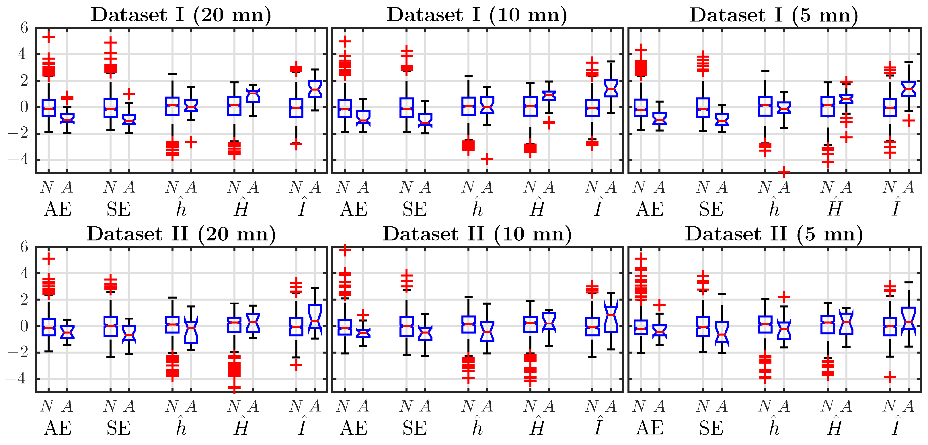
We compute the five features: ApEn, SampEn, , and for normal and acidotic (abnormal) subjects in Datasets I and II using data from the last mn before delivery, which are the most crucial. We use the classical values and for embedding dimensions. To compare the performance, we present the box plots of the five normalized (zero-mean, unit-variance) estimates in the left column of Figure 1.
For Dataset I, the average of ApEn and SampEn for acidotic subjects is smaller than for normal subjects, while the average of the Shannon entropy rate does not show any tendency. This is surprising as one might have expected for a behavior similar to ApEn and SampEn (see Section 3.3). Average values of and are larger for acidotic subjects.
The larger value of Shannon entropy H indicates that the acidotic FHR signals contain more information. The larger value of AMI indicates a stronger dependence structure in the dynamics of abnormal subjects.
For subjects in Dataset II, it is harder to find any tendency by looking at the average values.
Features performance:
Fetal acidosis detection performance is assessed with the p-value given by the classical Wilcoxon rank sum test. This non-parametric test of the null hypothesis, which corresponds to identical medians of the distributions of estimates in the normal and abnormal classes, is reported in Table 1.
We have added one ⋆ symbol when the p-value is less than 0.05, two when less than 0.01. We see that for Dataset I, ApEn, SampEn, and for discriminate normal and acidotic subjects, while does not. Out of the three estimates (ApEn, SampEn, ) based on entropy rates, the nearest-neighbors one for Shannon entropy rate is the poorest, although its decomposition into Shannon entropy (static one-point information) and AMI (which includes dynamic information) leads to two satisfying estimates Figure 1 and Table 1 both show that the best performing estimators are SampEn and . In Dataset II, although all features performs more poorly than in Dataset I, SampEn and AMI are again the best ones, with a p-value lower than 0.05. We focus on these two features in the following.
Receiver operating characteristics:
To compare the two best performing features, SampEn and AMI, we plot receiver operating characteristics (ROC) curves in Figure 2, both for Datasets I and II, using data from the last mn before delivery.
For Dataset I, AMI better discriminates acidotic subjects from normal ones. For Dataset II, AMI discrimination is only slightly better than SampEn. The area under the curve (AUC) of the ROC of the features is reported in Table 1, with bold font indicating the estimator with the largest AUC. Performance is much worse in Dataset II than in Dataset I: the AUC is reduced. Nevertheless, AMI is always the better performing estimator (its AUC reduces from to ), followed by SampEn (AUC reducing from to ).
4.2. Effect of Window Size on Performance
We investigate the robustness of the detection performance when the window size T is reduced, using data from and five minutes. Results are reported in Figure 1 and Table 2.
p-values and AUC both indicate that and SampEn provide robust discrimination in Dataset I even when the observation length is reduced. Again, performs better: its AUC is reduced from 0.84 to 0.83 when T is reduced from 20 mn to 5 mn, where the AUC of SampEn is reduced from 0.79 to 0.72. In Dataset II, once again, performance degrades, but AMI is still better at discriminating acidotic from normal subjects. In the following, we focus on AMI estimates only.
4.3. Effect of the Embedding Dimensions on the (Fetal Acidosis Detection) Performance of AMI
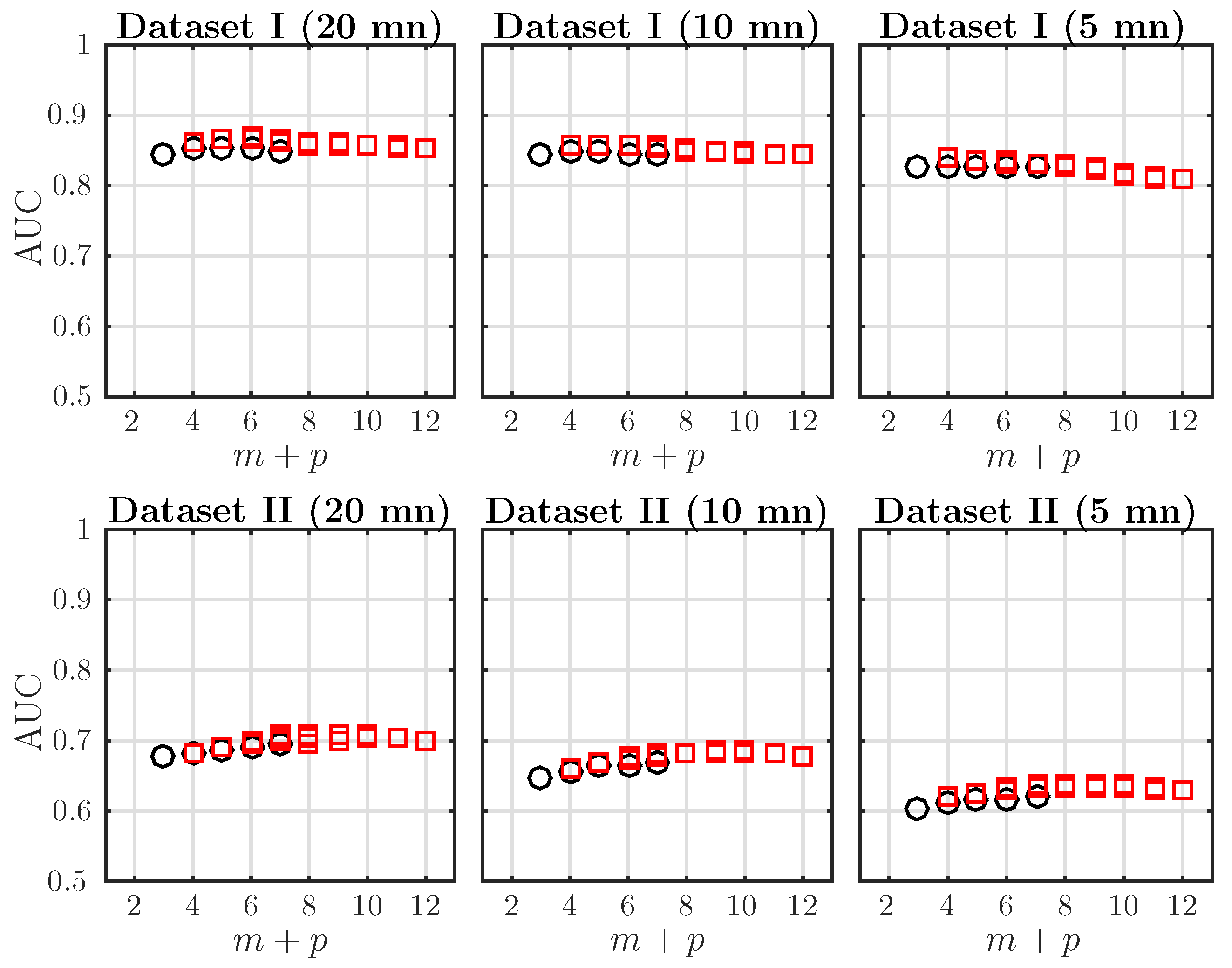
In order to improve the acidosis detection performance of the AMI, especially in Dataset II, we increase the embedding dimensions m and p used in computing . This way, we probe a higher order dependence structure in the dynamics. Because of the symmetry of AMI (Equation (10)) and aiming at probing the effect of increasing either m or p, we plot the AUC of ROC as a function of only. The dependence of AMI on is much smaller and not reported here. These computations have been done with a larger value in the k-NN algorithms, in order to accommodate the possibly large embedding dimensions ( up to 12). Results are presented in Figure 3.
For a fixed window size, the AUC increases when increases and reaches a maximum; it then remains constant or decreases slightly. This behavior is observed in both Datasets I and II and for any window size mn. Varying T dos not seem to change the location of the maximum of the AUC in a given dataset. The optimal embedding dimension is in Dataset I and in Dataset II. This hints at a difference in the dynamics of the FHR in the two datasets. Because both bias and computation time increase with the total dimensionality [57], the maximal embedding is restricted to . A reduction of the AUC is observed when the analysis window is reduced, but this is only significant for Dataset II.
We reported in Table 2 the AUC and p-values of the AMI for two embedding dimensions: and , for Datasets I and II and several window sizes. The best performing estimator is indicated in bold. For all observation windows and for the two datasets, achieves the best performance. Their AUC is always larger than the one obtained using SampEn or AMI with and .
4.4. Dynamical Analysis
We now explore how long before delivery the AMI can diagnose fetal acidosis on an FHR signal. To do so, we do not restrict our analysis to the last data points before delivery, but we apply it to an ensemble of windows scanning the first and second stages of labor. We examine the dynamics of , the best performing feature, for both normal and abnormal subjects.
4.4.1. Dataset I: Rapid Delivery
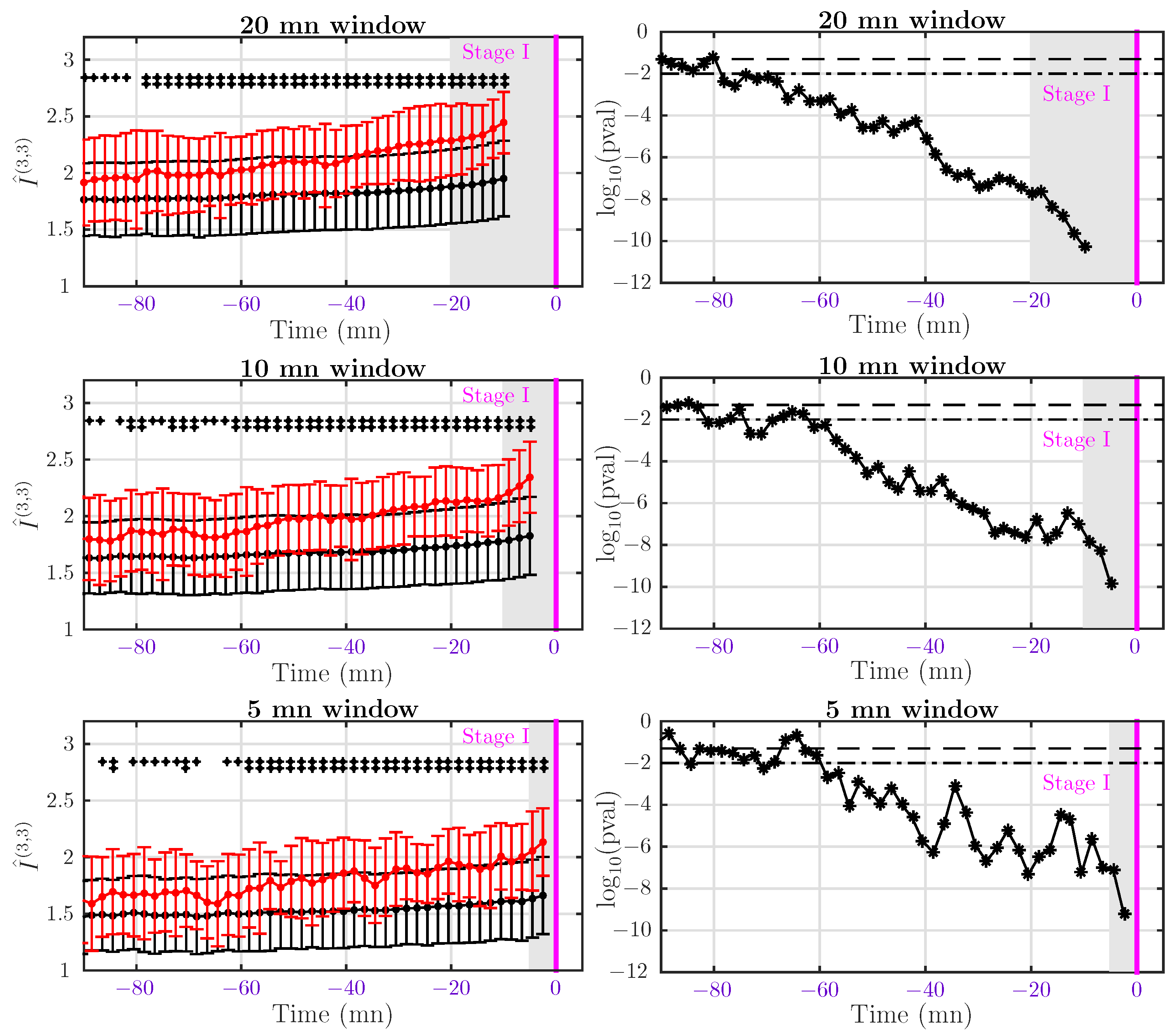
In this first section, we focus on Dataset I and probe Stage 1, including early labor, active labor and transition. Using the time at which Stage 1 ends as a reference (setting it at ), we compute for each subject in a set of time windows , of fixed size T ending at mn, so separated by 2 mn. We perform this analysis for three window sizes mn. The value of AMI computed in the i-th window is then assigned to time , at the center of the interval. By construction of Dataset I, delivery occurs less than 15 min after pushing started and can be as short as 1 mn, so we completely discard data from Stage 2. We then average the values of AMI over the population of normal subjects and over the population of acidotic subjects, respectively. Results, including p-values, are presented in Figure 4.
A first observation is that AMI is always larger for acidotic subjects than for normal subjects. As labor progresses, AMI increases in both populations, but the increase is stronger for acidotic subjects. As a consequence, the p-value of the test decreases clearly, so the feature performs better and better when approaching delivery. Detection of acidosis using the AMI feature and mn can be obtained in Dataset I as early as 80 min before entering the second stage. Using shorter windows, mn or 5 mn, detection is still reliable as early as one hour before Stage 2. We interpret this reduced forecast of acidosis detection in Dataset I as a direct consequence of the reduction of the statistics when the window size T is reduced.
4.4.2. Dataset II: Delivery after Pushing More Than 15 mn
For Dataset II, we performed the same dynamical analysis as in the previous section, using the end of Stage 1 as the reference time (). Because there is now enough data in the pushing stage, we also perform the analysis of this stage using the delivery time () as the reference. All results are presented in Figure 5.
At the end of Stage 1, we observe again that AMI is larger for acidotic subjects than for normal ones, but the difference is not significant in this group (see the corresponding p-value on the right of Figure 5). The situation is identical at the end of Stage 2, although we obtain a lower p-value in some windows. The p-value does not decrease clearly when approaching delivery time, as it was in Dataset I, see Figure 4. For subjects in Dataset II, it is very difficult to make an early detection of acidosis. However, we observe in Figure 5 that the average AMI is significantly larger at the end of Stage 2 than at the end of Stage 1. The increase of AMI is larger for abnormal subjects.
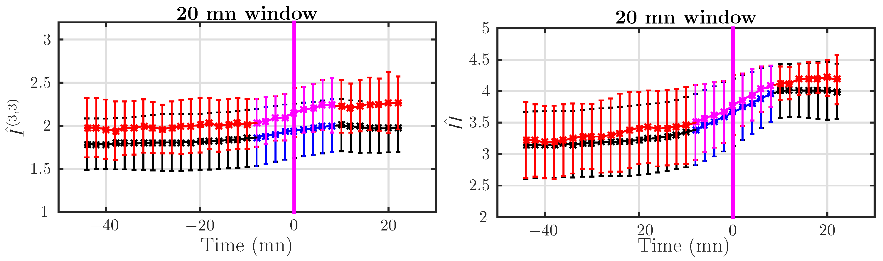
To examine more precisely the dynamical increase of AMI, especially when entering Stage 2, we computed over an ensemble of windows of size mn spanning continuously a large time interval that includes the end of the active labor and the beginning of the pushing stage. Results are reported in Figure 6.
We see a continuous increase of AMI values when evolving from Stage 1 to Stage 2. The increase is more important for abnormal subjects, which corroborates the findings in Figure 5. For smaller window sizes, the situation is less clear.
We also studied the dynamical evolution of the Shannon entropy estimate , which, together with the AMI, combines into the Shannon entropy rate (see Equation (11)). Changes in the Shannon entropy H indicate changes in the probability density of the signal. Results are presented in Figure 6, side by side with the AMI. We observe a dramatic rise of the value of when subjects evolve from Stage 1 to Stage 2. This increase is clearly observed for normal and abnormal subjects. No significant difference between normal and acidotic subjects is observed for this static quantity. The start of pushing implies a strong deformation of the probability density of the FHR, indicating strong perturbations of the FHR, for both normal and acidotic subjects.
5. Discussion, Conclusions and Perspectives
We now discuss the interpretation of Shannon entropy and AMI measurements in different stages of labor. The fetuses are classified as normal or acidotic depending on a post-delivery pH measurement, which gives a diagnosis of acidosis at delivery only. There is no information on the health of the fetuses during labor.
The physiological interpretation of a feature, and especially its relation to specific FHR patterns, e.g., like those detailed in [2,58], is a difficult task that is only scarcely reported in the literature [59,60]. In this article, we have averaged our results over large numbers of (normal or acidotic) subjects, which jeopardizes any precise interpretation in terms of a specific FHR pattern that may appear only intermittently.
5.1. Acidosis Detection in the First Stage
We can nevertheless suggest that the value of the Shannon entropy H is related to the frequency of decelerations in the FHR signals. Indeed, Shannon entropy strongly depends on the standard deviation of the signal (e.g., see Equation (15)), which in turn depends on the variability in the observation window. A larger number of decelerations in the observation window deforms the PDF of the FHR signal by increasing its lower tail; in particular, this increases the width of the PDF and hence increases the standard deviation and the Shannon entropy. This explains our findings in Figure 1 (for Dataset I).
When acidosis develops in the first stage of labor, the Shannon auto-mutual information estimator significantly outperforms all other quantities both in terms of p-value and AUC. The performance of AMI is robust when tuning either the size of the observation, and hence the number of points in the data, and the embedding dimensions . In addition, the performance slightly increases when the total embedding dimension increases; although one has to care about the curse of dimensionality.
For abnormal subjects from Dataset II, AMI is not able to detect acidosis using data from Stage 1. This suggests that acidosis develops later, in the second stage of labor.
For all datasets, AMI computed with s is always larger for acidotic subjects than for normal subjects. This is in agreement with results obtained with ApEn and SampEn, which are both lower for acidotic subjects. This shows that FHR classified as abnormal have a stronger dependence structure at a small scale than normal ones. We can relate this increase of the dependence structure of acidotic FHR to the short-term variability and to its coupling with particular large-scale patterns. For example, a sinusoidal FHR pattern [2], especially if its duration is long, should give a larger value of the AMI, because its large-scale dynamics is highly predictable. As another example, we expect variable decelerations (with an asymmetrical V-shape) and late decelerations (with a symmetrical U-shape and/or reduced variability) to impact AMI differently. Of course, the choice of the embedding parameter is then crucial, and this is currently under investigation.
AMI and entropy rates depend on the dynamics as they operate on time-embedded vectors. AMI focuses on nonlinear temporal dynamics, while being insensitive to the dominant static information. AMI is independent of the standard deviation, which on the contrary contributes strongly to the Shannon entropy. This explains why AMI performs better than entropy rate estimates, such as ApEn, SampEn and , which depend also on the standard deviation.
5.2. Acidosis Detection in Second Stage
The results reported for Stage 2 show a severe decrease in the performance of the five estimated quantities. Analyzing Stage 2 is far more challenging than analyzing Stage 1, which suggests that temporal dynamics in Stage 2 differ notably from those of Stage 1 [38] or simply that our database does not contain enough acidotic subjects in that case. achieves the best performance in terms of p-value and AUC; this clearly underlines that the analysis of nonlinear temporal dynamics is critical for fetal acidosis detection in Stage 2. As in Stage 1, the AMI is always larger in Stage 2 for acidotic subjects than for normal subjects.
Although the Shannon entropy computed from the last 20 mn of Stage 2 before delivery does not show a clear tendency in Figure 1 for Dataset II, looking at Figure 6 clearly shows that increases as labor progresses: this is probably related to the average increase of the number of decelerations, which is expected in both the normal and acidotic population.
SampEn is also able to perform discrimination in Stage 2. From these observations, one may envision the definition of a new estimator that would measure the auto-mutual information using the Rényi order-two entropy by applying Equation (12). Nevertheless, it should be emphasized that Rényi order-q entropy is lacking the chain rule of conditional probabilities as soon as , which may jeopardize any practical use of such an estimator.
5.3. Probing the Dynamics
Increasing the total embedding dimensions in AMI improves the performance in the detection of acidotic subjects, in both the first and second stages. The best performance is found for different total embedding dimension in the two datasets. This suggests that FHR dynamics is different in each stage.
As seen in Equation (11), the Shannon entropy rate can be split into two contributions: one that depends only on static properties (the Shannon entropy, estimated by ) and one that involves the signal dynamics (the auto-mutual information, estimated by ). By following the time evolution of these two parts, we were able to relate Shannon entropy with the evolution of the labor and AMI not only with the evolution of the labor, but also with possible acidosis. Looking at subjects for which the pushing phase is longer than 15 mn, it clearly appears that all fetuses are affected by the pushing, as evidenced by a large increase of the Shannon entropy and a small increase of AMI. Additionally, the increase of AMI is steeper for abnormal subjects than for normal ones, which may indicate different reactions to the pushing and can be related to specific pathological FHR patterns. When the pushing stage is long (Dataset II), fetuses reported as acidotic do not show any sign of acidosis until prolonged pushing. These fetuses appear as normal until delivery is near.
When acidosis develops during the first stage of labor, in Dataset I, we observe clearly that while AMI increases steadily till delivery for healthy fetuses, it increases faster for acidotic ones. This suggests that acidotic fetuses in Dataset I react to early labor, as early as one hour before pushing starts. This could not only indicate that some fetuses are prone to acidosis, but also may pave the way for an early detection of acidosis in this case.
Acknowledgments
This work was supported by the LabEx iMUST (Institute of MUltiscale Science and Technology) under grant ANR-10-LABX-0064 of Université de Lyon, within the program “Investissements d’Avenir” (grant ANR-11-IDEX-0007) operated by the French National Research Agency (ANR).
Author Contributions
Muriel Doret and Patrice Abry conceived the database; Nicolas B. Garnier developed the theoretical tools; Stéphane G. Roux and Nicolas B. Garnier designed the analysis tools; Carlos Granero-Belinchon, Stéphane G. Roux and Nicolas B. Garnier analyzed the data; Carlos Granero-Belinchon, Stéphane G. Roux, Patrice Abry and Nicolas B. Garnier wrote the paper.
Conflicts of Interest
The authors declare no conflict of interest.
References
- Chandraharan, E.; Arulkumaran, S. Prevention of birth asphyxia: Responding appropriately to cardiotocograph (CTG) traces. Best Pract. Res. Clin. Obstet. Gynaecol. 2007, 21, 609–624. [Google Scholar] [CrossRef] [PubMed]
- Ayres-de-Campos, D.; Spong, C.Y.; Chandraharan, E.; The FIGO Intrapartum Fetal Monitoring Expert Consensus Panel. FIGO consensus guidelines on intrapartum fetal monitoring: Cardiotocography. Int. J. Gynaecol. Obstet. 2015, 131, 13–24. [Google Scholar] [CrossRef] [PubMed] [Green Version]
- Rooth, G.; Huch, A.; Huch, R. Guidelines for the Use of Fetal Monitoring. Int. J. Gynaecol. Obstet. 1987, 25, 159–167. [Google Scholar]
- Hruban, L.; Spilka, J.; Chudáček, V.; Janků, P.; Huptych, M.; Burša, M.; Hudec, A.; Kacerovský, M.; Koucký, M.; Procházka, M.; et al. Agreement on intrapartum cardiotocogram recordings between expert obstetricians. J. Eval. Clin. Pract. 2015, 21, 694–702. [Google Scholar] [CrossRef] [PubMed]
- Alfirevic, Z.; Devane, D.; Gyte, G.M. Continuous cardiotocography (CTG) as a form of electronic fetal monitoring (EFM) for fetal assessment during labor. Cochrane Database Syst. Rev. 2006, 3. [Google Scholar] [CrossRef]
- Spilka, J.; Chudáček, V.; Koucký, M.; Lhotská, L.; Huptych, M.; Janků, P.; Georgoulas, G.; Stylios, C. Using nonlinear features for fetal heart rate classification. Biomed. Signal Process. Control 2012, 7, 350–357. [Google Scholar] [CrossRef]
- Haritopoulos, M.; Illanes, A.; Nandi, A. Survey on Cardiotocography Feature Extraction Algorithms for Fetal Welfare Assessment. In XIV Mediterranean Conference on Medical and Biological Engineering and Computing (MEDICON); Kyriacou, E., Christofides, S., Pattichis, C.S., Eds.; Springer International Publishing: Cham, Switzerland, 2016; pp. 1193–1198. [Google Scholar]
- Akselrod, S.; Gordon, D.; Ubel, F.A.; Shannon, D.C.; Berger, A.C.; Cohen, R.J. Power spectrum analysis of heart rate fluctuation: A quantitative probe of beat-to-beat cardiovascular control. Science 1981, 213, 220–222. [Google Scholar] [CrossRef] [PubMed]
- Gonçalves, H.; Rocha, A.P.; de Campos, D.A.; Bernardes, J. Linear and nonlinear fetal heart rate analysis of normal and acidemic fetuses in the minutes preceding delivery. Med. Biol. Eng. Comput. 2006, 44, 847–855. [Google Scholar] [CrossRef] [PubMed]
- Van Laar, J.; Porath, M.; Peters, C.; Oei, S. Spectral analysis of fetal heart rate variability for fetal surveillance: Review of the literature. Acta Obstet. Gynecol. Scand. 2008, 87, 300–306. [Google Scholar] [CrossRef] [PubMed]
- Siira, S.M.; Ojala, T.H.; Vahlberg, T.J.; Rosén, K.G.; Ekholm, E.M. Do spectral bands of fetal heart rate variability associate with concomitant fetal scalp pH? Early Hum. Dev. 2013, 89, 739–742. [Google Scholar] [CrossRef] [PubMed]
- Francis, D.P.; Willson, K.; Georgiadou, P.; Wensel, R.; Davies, L.; Coats, A.; Piepoli, M. Physiological basis of fractal complexity properties of heart rate variability in man. J. Physiol. 2002, 542, 619–629. [Google Scholar] [CrossRef] [PubMed]
- Doret, M.; Helgason, H.; Abry, P.; Gonçalvés, P.; Gharib, C.; Gaucherand, P. Multifractal analysis of fetal heart rate variability in fetuses with and without severe acidosis during labor. Am. J. Perinatol. 2011, 28, 259–266. [Google Scholar] [CrossRef] [PubMed]
- Doret, M.; Spilka, J.; Chudáček, V.; Gonçalves, P.; Abry, P. Fractal Analysis and Hurst Parameter for intrapartum fetal heart rate variability analysis: A versatile alternative to Frequency bands and LF/HF ratio. PLoS ONE 2015, 10, e0136661. [Google Scholar] [CrossRef] [PubMed] [Green Version]
- Echeverria, J.C.; Hayes-Gill, B.R.; Crowe, J.A.; Woolfson, M.S.; Croaker, G.D.H. Detrended fluctuation analysis: A suitable method for studying fetal heart rate variability? Physiol. Meas. 2004, 25, 763–774. [Google Scholar] [CrossRef] [PubMed]
- Chudáček, V.; Anden, J.; Mallat, S.; Abry, P.; Doret, M. Scattering Transform for Intrapartum Fetal Heart Rate Variability Fractal Analysis: A Case-Control Study. IEEE Trans. Biomed. Eng. 2014, 61, 1100–1108. [Google Scholar] [CrossRef] [PubMed]
- Magenes, G.; Signorini, M.G.; Arduini, D. Classification of cardiotocographic records by neural networks. Proc. IEEE-INNS-ENNS Int. Jt. Conf. Neural Netw. 2000, 3, 637–641. [Google Scholar]
- Pincus, S.M.; Viscarello, R.R. Approximate entropy: A regularity measure for fetal heart rate analysis. Obstet. Gynecol. 1992, 79, 249–255. [Google Scholar] [PubMed]
- Pincus, S. Approximate entropy (ApEn) as a complexity measure. Chaos 1995, 5, 110–117. [Google Scholar] [CrossRef] [PubMed]
- Lake, D.E.; Richman, J.S.; Griffin, M.P.; Moorman, J.R. Sample entropy analysis of neonatal heart rate variability. Am. J. Physiol. Regul. Integr. Comp. Physiol. 2002, 283, R789–R797. [Google Scholar] [CrossRef] [PubMed]
- Georgieva, A.; Payne, S.J.; Moulden, M.; Redman, C.W.G. Artificial neural networks applied to fetal monitoring in labor. Neural Comput. Appl. 2013, 22, 85–93. [Google Scholar] [CrossRef]
- Czabanski, R.; Jezewski, J.; Matonia, A.; Jezewski, M. Computerized analysis of fetal heart rate signals as the predictor of neonatal acidemia. Expert Syst. Appl. 2012, 39, 11846–11860. [Google Scholar] [CrossRef]
- Warrick, P.; Hamilton, E.; Precup, D.; Kearney, R. Classification of normal and hypoxic fetuses from systems modeling of intrapartum cardiotocography. IEEE Trans. Biomed. Eng. 2010, 57, 771–779. [Google Scholar] [CrossRef] [PubMed]
- Spilka, J.; Frecon, J.; Leonarduzzi, R.; Pustelnik, N.; Abry, P.; Doret, M. Sparse Support Vector Machine for Intrapartum Fetal Heart Rate Classification. IEEE J. Biomed. Health Inf. 2016, 21, 1–8. [Google Scholar] [CrossRef] [PubMed]
- Dawes, G.; Moulden, M.; Sheil, O.; Redman, C. Approximate entropy, a statistic of regularity, applied to fetal heart rate data before and during labor. Obstet. Gynecol. 1992, 80, 763–768. [Google Scholar] [PubMed]
- Richman, J.S.; Moorman, J.R. Physiological time-series analysis using approximate entropy and sample entropy. Am. J. Physiol. Heart Circ. Physiol. 2000, 278, H2039–H2049. [Google Scholar] [PubMed]
- Grünwald, P.; Vitányistard, P. Kolmogorov complexity and information theory. With an interpretation in terms of questions and answers. J. Log. Lang. Inf. 2003, 12, 497–529. [Google Scholar] [CrossRef]
- Lake, D.E. Renyi entropy measures of heart rate Gaussianity. IEEE Trans. Biomed. Eng. 2006, 53, 21–27. [Google Scholar] [CrossRef] [PubMed]
- Grassberger, P.; Procaccia, I. Estimation of the Kolmogorov-entropy from a Chaotic Signal. Phys. Rev. A 1983, 28, 2591–2593. [Google Scholar] [CrossRef]
- Kozachenko, L.F.; Leonenko, N.N. Sample Estimate of the Entropy of a Random Vector. Probl. Inf. Transm. 1987, 23, 95–101. [Google Scholar]
- Porta, A.; Bari, V.; Bassani, T.; Marchi, A.; Tassin, S.; Canesi, M.; Barbic, F.; Furlan, R. Entropy-based complexity of the cardiovascular control in Parkinson disease: Comparison between binning and k-nearest-neighbor approaches. In Proceedings of the IEEE Engineering in Medicine and Biology Society (EMBC), Osaka, Japan, 3–7 July 2013; pp. 5045–5048. [Google Scholar]
- Spilka, J.; Roux, S.; Garnier, N.; Abry, P.; Goncalves, P.; Doret, M. Nearest-neighbor based wavelet entropy rate measures for intrapartum fetal heart rate variability. In Proceedings of the IEEE Engineering in Medicine and Biology Society (EMBC), Chicago, IL, USA, 26–30 August 2014; pp. 2813–2816. [Google Scholar]
- Xiong, W.; Faes, L.; Ivanov, P.C. Entropy measures, entropy estimators, and their performance in quantifying complex dynamics: Effects of artifacts, nonstationarity, and long-range correlations. Phys. Rev. E 2017, 95, 062114. [Google Scholar] [CrossRef] [PubMed]
- Costa, A.; Ayres-de Campos, D.; Costa, F.; Santos, C.; Bernardes, J. Prediction of neonatal acidemia by computer analysis of fetal heart rate and ST event signals. Am. J. Obstet. Gynecol. 2009, 201, 464.e1–464.e6. [Google Scholar] [CrossRef] [PubMed]
- Georgieva, A.; Papageorghiou, A.T.; Payne, S.J.; Moulden, M.; Redman, C.W.G. Phase-rectified signal averaging for intrapartum electronic fetal heart rate monitoring is related to acidaemia at birth. BJOG 2014, 121, 889–894. [Google Scholar] [CrossRef] [PubMed]
- Spilka, J.; Abry, P.; Goncalves, P.; Doret, M. Impacts of first and second labor stages on Hurst parameter based intrapartum fetal heart rate analysis. In Proceedings of the IEEE Computing in Cardiology Conference (CinC), Cambridge, MA, USA, 7–10 September 2014; pp. 777–780. [Google Scholar]
- Lim, J.; Kwon, J.Y.; Song, J.; Choi, H.; Shin, J.C.; Park, I.Y. Quantitative comparison of entropy analysis of fetal heart rate variability related to the different stages of labor. Early Hum. Dev. 2014, 90, 81–85. [Google Scholar] [CrossRef] [PubMed]
- Spilka, J.; Leonarduzzi, R.; Chudáček, V.; Abry, P.; Doret, M. Fetal Heart Rate Classification: First vs. Second Stage of Labor. In Proceedings of the 8th International Workshop on Biosignal Interpretation, Osaka, Japan, 1–3 November 2016. [Google Scholar]
- Granero-Belinchon, C.; Roux, S.; Garnier, N.; Abry, P.; Doret, M. Mutual information for intrapartum fetal heart rate analysis. In Proceedings of the IEEE Engineering in Medicine and Biology Society (EMBC), Seogwipo, South Korea, 11–15 July 2017. [Google Scholar]
- Costa, M.; Goldberger, A.L.; Peng, C.K. Multiscale entropy analysis of complex physiologic time series. Phys. Rev. Lett. 2002, 89, 068102. [Google Scholar] [CrossRef] [PubMed]
- Doret, M.; Massoud, M.; Constans, A.; Gaucherand, P. Use of peripartum ST analysis of fetal electrocardiogram without blood sampling: A large prospective cohort study. Eur. J. Obstet. Gynecol. Reprod. Biol. 2011, 156, 35–40. [Google Scholar] [CrossRef] [PubMed]
- Takens, F. Detecting strange attractors in turbulence. Dyn. Syst. Turbul. 1981, 4, 366–381. [Google Scholar]
- Shannon, C. A Mathematical Theory of Communication. Bell Syst. Tech. J. 1948, 27, 388–427. [Google Scholar] [CrossRef]
- Rényi, A. On measures of information and entropy. In Proceedings of the Fourth Berkeley Symposium on Mathematical Statistics and Probability, Berkeley, CA, USA, 20 June–30 July 1960; pp. 547–561. [Google Scholar]
- Kullback, S.; Leibler, R. On information and sufficiency. Ann. Math. Stat. 1951, 22, 79–86. [Google Scholar] [CrossRef]
- Gomez, C.; Lizier, J.; Schaum, M.; Wollstadt, P.; Grutzner, C.; Uhlhaas, P.; Freitag, C.; Schlitt, S.; Bolte, S.; Hornero, R.; et al. Reduced predictable information in brain signals in autism spectrum disorder. Front. Neuroinf. 2014, 8. [Google Scholar] [CrossRef] [PubMed]
- Faes, L.; Porta, A.; Nollo, G. Information Decomposition in Bivariate Systems: Theory and Application to Cardiorespiratory Dynamics. Entropy 2015, 17, 277–303. [Google Scholar] [CrossRef]
- Granero-Belinchon, C.; Roux, S.G.; Garnier, N.B. Scaling of information in turbulence. EPL 2016, 115, 58003. [Google Scholar] [CrossRef]
- Eckmann, J.P.; Ruelle, D. Ergodic-Theory of Chaos and Strange Attractors. Rev. Mod. Phys. 1985, 57, 617–656. [Google Scholar] [CrossRef]
- Pincus, S.M. Approximate Entropy as a Measure of System-complexity. Proc. Natl. Acad. Sci. USA 1991, 88, 2297–2301. [Google Scholar] [CrossRef] [PubMed]
- Krstacic, G.; Krstacic, A.; Martinis, M.; Vargovic, E.; Knezevic, A.; Smalcelj, A.; Jembrek-Gostovic, M.; Gamberger, D.; Smuc, T. Non-linear analysis of heart rate variability in patients with coronary heart disease. Comput. Cardiol. 2002, 29, 673–675. [Google Scholar]
- Richman, J.; Moorman, R. Time series analysis using approximate entropy and sample entropy. Biophys. J. 2000, 78, 218A. [Google Scholar]
- Lake, D. Improved entropy rate estimation in physiological data. In Proceedings of the IEEE Engineering in Medicine and Biology Society (EMBC), Boston, MA, USA, 30 August–3 September 2011; pp. 1463–1466. [Google Scholar]
- Jaynes, E.T. Information Theory and Statistical Mechanics. Phys. Rev. 1957, 106, 620–630. [Google Scholar] [CrossRef]
- Singh, H.; Misra, N.; Hnizdo, V.; Fedorowicz, A.; Demchuk, E. Nearest neighbor estimates of entropy. Am. J. Math. Manag. Sci. 2003, 23, 301–321. [Google Scholar] [CrossRef]
- Kraskov, A.; Stogbauer, H.; Grassberger, P. Estimating mutual information. Phys. Rev. E 2004, 69, 066138. [Google Scholar] [CrossRef] [PubMed]
- Gao, W.; Oh, S.; Viswanath, P. Demystifying Fixed k-Nearest Neighbor Information Estimators. In Proceedings of the IEEE Information Theory (ISIT), Aachen, Germany, 25–30 June 2017. [Google Scholar]
- Freeman, R. Problems with intrapartum fetal heart rate monitoring interpretation and patient management. Obstet. Gynecol. 2002, 100, 813–826. [Google Scholar] [PubMed]
- Signorini, M.; Magenes, G.; Cerutti, S.; Arduini, D. Linear and nonlinear parameters for the analysis of fetal heart rate signal from cardiotocographic recordings. IEEE Trans. Biomed. Eng. 2003, 50, 365–374. [Google Scholar] [CrossRef] [PubMed]
- Gonçalves, H.; Henriques-Coelho, T.; Bernardes, J.; Rocha, A.; Nogueira, A.; Leite-Moreira, A. Linear and nonlinear heart-rate analysis in a rat model of acute anoxia. Physiol. Meas. 2008, 29, 1133–1143. [Google Scholar] [CrossRef] [PubMed]
Figure 1.
Box plot-based comparisons of the five different (normalized) estimates (ApEn (AE), SampEn (SE), Shannon entropy rate (), Shannon entropy () and auto-mutual information (AMI) ()) for normal (N) and pathological (A for “abnormal”) subjects, for Dataset I (top) and Dataset II (bottom). Each column corresponds to a different window size: 20 mn, 10 mn and 5 mn. All features are computed with , .

Figure 2.
Receiver operating characteristics (ROC) curves for SampEn (black) and AMI estimator (red), for subjects in Datasets I (left) and II (right). , .
Figure 2.
Receiver operating characteristics (ROC) curves for SampEn (black) and AMI estimator (red), for subjects in Datasets I (left) and II (right). , .
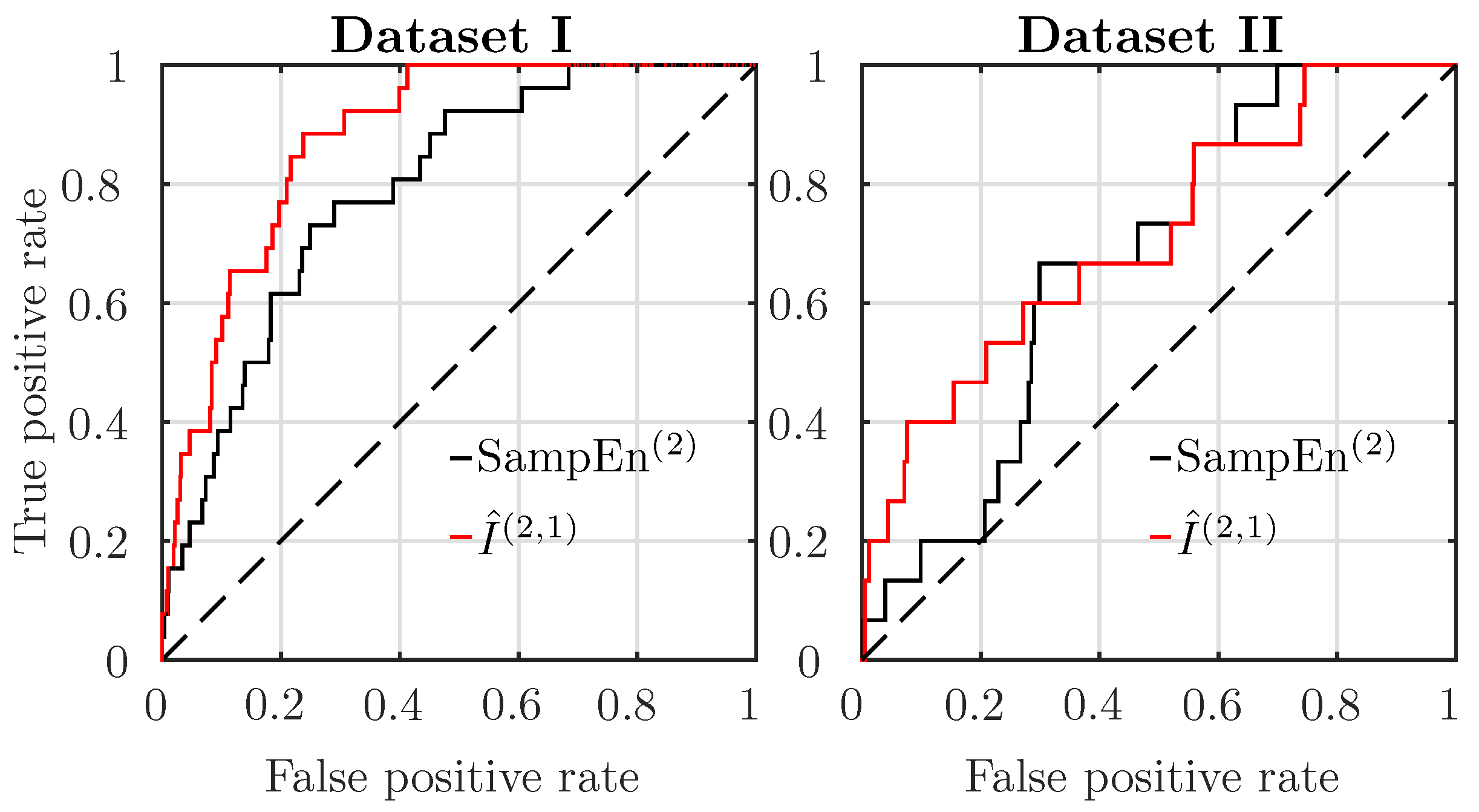
Figure 3.
AUC of ROC for as a function of the total embedding dimension , with , for time windows of size mn, for data in Dataset I (first line) and Dataset II (second line). Black circles indicate the special case corresponding to the classical definition of Shannon entropy rate (see Equation (11)). Red squares correspond to .

Figure 4.
Left: Average AMI for normal (black) and abnormal (red) subjects in Dataset I (delivery occurring less then 15 mn after pushing started). AMI is computed in windows of size mn (first line), 10 mn (second line) and 5 mn (third line) shifted by 2 mn. The vertical magenta line indicates the beginning of Stage 2 (pushing). Right: Corresponding p-value. A single black + symbol in the AMI plot indicates a p-value lower than 0.05, two ++ indicate a p-value lower than 0.01. The gray-shaded region represents the time window used to compute the last value of AMI.

Figure 5.
Left: Average AMI for normal (black) and abnormal (red) subjects in Dataset II (delivery occurring more then 15 mn after pushing started). AMI is computed in windows of size mn (first line), 10 mn (second line) and 5 mn (third line) shifted by 2 mn. The vertical magenta line indicates the beginning of Stage 2 (pushing), and the vertical blue line indicates delivery. Right: Corresponding p-value. Black + symbols in the AMI plot indicate a p-value lower than 5% (+) or lower than 1% (++). The gray-shaded region represents the time window used to compute the last value of AMI.

Figure 6.
Average behavior of AMI (left) and Shannon entropy (right) for normal (black) and acidotic (red) subjects in Dataset II (delivery occurring more than 15 mn after pushing started). Quantities are computed in windows of size mn. The vertical magenta line indicates the beginning of Stage 2 (pushing). We have used a different color code for windows spanning both Stages 1 and 3: blue for normal subjects and magenta for acidotic ones.


Table 1.
Area under Receiver Operational Characteristics curves (as shown in Figure 2) and p-value obtained from the Wilcoxon rank-sum test, for each of the five different estimates, all with .
Table 1.
Area under Receiver Operational Characteristics curves (as shown in Figure 2) and p-value obtained from the Wilcoxon rank-sum test, for each of the five different estimates, all with .
| Dataset I | Dataset II | |||
|---|---|---|---|---|
| AUC | p-Value | AUC | p-Value | |
| ApEn | 0.76 | 4.08 × 10⁻⁶ | 0.61 | 1.33 × 10⁻¹ |
| SampEn | 0.79 | 5.92 × 10⁻⁷ | 0.67 | 2.35 × 10⁻² ⋆ |
| 0.50 | 9.75 × 10⁻¹ | 0.39 | 1.36 × 10⁻¹ | |
| 0.76 | 8.36 × 10⁻⁶ | 0.56 | 4.23 × 10⁻¹ | |
| 0.84 | 2.00 × 10⁻⁹ | 0.68 | 1.69 × 10⁻² ⋆ | |
Table 2.
AUC and p-value of Wilcoxon test of SampEn and AMI in datasets I and II using data from the last 20, 10 or 5 mn before delivery.
Table 2.
AUC and p-value of Wilcoxon test of SampEn and AMI in datasets I and II using data from the last 20, 10 or 5 mn before delivery.
| SampEn | |||||||
|---|---|---|---|---|---|---|---|
| AUC | p-Value | AUC | p-Value | AUC | p-Value | ||
| Dataset I | 20 mn | 0.79 | 5.92 × 10⁻⁷ | 0.84 | 2.00 × 10⁻⁹ | 0.88 | 5.46 × 10⁻¹¹ |
| 10 mn | 0.76 | 1.22 × 10⁻⁷ | 0.84 | 2.22 × 10⁻⁹ | 0.87 | 1.40 × 10⁻¹⁰ | |
| 5 mn | 0.72 | 1.97 × 10⁻⁷ | 0.83 | 7.47 × 10⁻⁹ | 0.86 | 6.26 × 10⁻¹⁰ | |
| Dataset II | 20 mn | 0.67 | 2.35 × 10⁻² ⋆ | 0.68 | 1.69 × 10⁻² ⋆ | 0.71 | 5.36 × 10⁻³ |
| 10 mn | 0.62 | 1.56 × 10⁻² ⋆ | 0.64 | 5.87 × 10⁻² | 0.68 | 1.66 × 10⁻² ⋆ | |
| 5 mn | 0.62 | 5.16 × 10⁻² | 0.60 | 1.70 × 10⁻¹ | 0.64 | 7.29 × 10⁻² | |
© 2017 by the authors. Licensee MDPI, Basel, Switzerland. This article is an open access article distributed under the terms and conditions of the Creative Commons Attribution (CC BY) license (http://creativecommons.org/licenses/by/4.0/).
Share and Cite
MDPI and ACS Style
Granero-Belinchon, C.; Roux, S.G.; Abry, P.; Doret, M.; Garnier, N.B. Information Theory to Probe Intrapartum Fetal Heart Rate Dynamics. Entropy 2017, 19, 640. https://doi.org/10.3390/e19120640
AMA Style
Granero-Belinchon C, Roux SG, Abry P, Doret M, Garnier NB. Information Theory to Probe Intrapartum Fetal Heart Rate Dynamics. Entropy. 2017; 19(12):640. https://doi.org/10.3390/e19120640
Chicago/Turabian StyleGranero-Belinchon, Carlos, Stéphane G. Roux, Patrice Abry, Muriel Doret, and Nicolas B. Garnier. 2017. "Information Theory to Probe Intrapartum Fetal Heart Rate Dynamics" Entropy 19, no. 12: 640. https://doi.org/10.3390/e19120640
Note that from the first issue of 2016, this journal uses article numbers instead of page numbers. See further details here.