Sparse Coding Algorithm with Negentropy and Weighted ℓ1-Norm for Signal Reconstruction


Tianjin Key Laboratory of Optoelectronic Sensor and Sensing Network Technology, College of Electronic Information and Optical Engineering, Nankai University, Tianjin 300071, China
*
Author to whom correspondence should be addressed.
Entropy 2017, 19(11), 599; https://doi.org/10.3390/e19110599
Submission received: 20 September 2017
/
Revised: 24 October 2017
/
Accepted: 6 November 2017
/
Published: 8 November 2017
(This article belongs to the Section Information Theory, Probability and Statistics)
Abstract
:Compressive sensing theory has attracted widespread attention in recent years and sparse signal reconstruction has been widely used in signal processing and communication. This paper addresses the problem of sparse signal recovery especially with non-Gaussian noise. The main contribution of this paper is the proposal of an algorithm where the negentropy and reweighted schemes represent the core of an approach to the solution of the problem. The signal reconstruction problem is formalized as a constrained minimization problem, where the objective function is the sum of a measurement of error statistical characteristic term, the negentropy, and a sparse regularization term, -norm, for 0 < p < 1. The -norm, however, leads to a non-convex
optimization problem which is difficult to solve efficiently. Herein we treat the -norm as a
serious of weighted -norms so that the sub-problems become convex. We propose an optimized
algorithm that combines forward-backward splitting. The algorithm is fast and succeeds in exactly
recovering sparse signals with Gaussian and non-Gaussian noise. Several numerical experiments
and comparisons demonstrate the superiority of the proposed algorithm.
1. Introduction
Sparse signal reconstruction, or compressed sensing, is an emerging field in signal processing and communication [1,2,3,4,5,6]. The problem of recovering a sparse signal from a very low number of linear measurements arises in many real application fields, ranging from error correction and lost data recovery, to image acquisition and reconstruction. In general, an -dimensional sparse signal can be described by significant coefficients in an appropriate transform domain. In some cases, a signal which is non-sparse in time domain can be classified as a sparse one, as it shows sparsity in spatial domain or some appropriate transform domain, such as the frequency domain and Gabor transformed domain.
In this paper, the signals will be treated as real-valued functions having domains that are either continuous or discrete, and either infinite or finite. We will typically be concerned with normed vector spaces. In the case of a discrete, finite domain, the signals can be viewed as vectors in an -dimensional Euclidean space, denoted by . According to the compressed sensing theory, sparse signal reconstruction problem can be formalized as a constrained minimization problem, where the objective function defines the sparsity. The basic mathematical model is:
where is a known measurement matrix with and needs to satisfy the RIP condition. Any columns vectors are linearly independent [7]. is an available measurement vector. is an unknown noise vector. The sparse reconstruction problem can be cast as: given the measurement matrix , find the vector , whose nonzero components are only , with (such a vector will be called -sparse vector), from the measurements , by solving:
The most natural choice for is given by , where denotes the -norm, which counts the number of non-zero components in . With , however, the problem in (2) becomes a combinatorial optimization and is proven to be non-deterministic polynomial (NP)-hard [8]. Recent results have shown that the use of different sparsity inducing functions allows us to exactly and efficiently recover a sparse signal from a lower number of measurements [9,10,11]. For instance, -norm is introduced as a relaxation of the -norm, and the problem can be formulated by applying constraints on the signal model and introducing a cost function:
where is the -norm of , with . is the regularizing parameter which controls the sparsity.
Many algorithms have been developed to solve the problem in (3) in the literature [12,13,14,15,16,17,18,19,20], where the mean square error (MSE) [21] criterion based on second-order statistics has been employed for these algorithms, which show their optimality when is Gaussian noise. In practical applications, however the transmitted signals are distorted by not only Gaussian noise, but also other kinds of noise, such as burst noise and high noise. Burst noise is a type of discrete noise and consists of sudden interruptions. High noise has high energy, frequency or power. These noises have non-Gaussian characteristics. In such cases, the MSE criterion becomes less robust.
In this work, we focus on the problem of sparse signal reconstruction especially with non-Gaussian noise. This problem is formalized as a constrained minimization problem and verified by simulation. We propose a sparse coding algorithm in which the sparse signal is recovered by applying the negentropy [22] as the error measurement and -norm as the sparsity regularization. The -norm as sparsity constraint is not very commonly used due to its non-convexity. To solve the corresponding non-convex minimization problems, we treat -norm as a serious of weighted -norm and convert it to a series of convex optimizations. The negentropy, rather than the MSE, is used because of two folds of reasons. First, in the square error (SE) case, the minimization is on the cost function of the form MSE + -norm like Equation (3). Since SE is required to be as small as possible while the -norm is lower bounded by a finite value, the optimization cannot reach a very small SE value, so that leads a biased solution. In our case, the cost is negentropy + (weighted) -norm, the negentropy is required to be maximized and have finite value in the optimal state, so that an unbiased solution can be obtained. Second, negentropy can tolerate bigger, non-Gaussian noise on the zero-valued components so that the estimation for non-zero-valued components becomes more accurate. For efficient optimization, we propose an algorithm with two main steps: first we use the gradient-based maximization only to the negentropy; then we find a sparser solution within the neighborhood of what has been obtained in the gradient-based maximization. Such a strategy was termed in the literature as the forward-backward splitting (FOBOS) algorithm [23].
The proposed algorithm is distinguished from other related works in that we present a novel objective function for sparse signal recovery. The sparse signals can be estimated by applying the negentropy as the error measurement and weighted -norm as the sparsity regularization. An effective algorithm is provided, which has improved accuracy and convergence rate.
This paper is organized as follows: in Section 2 we recall the least absolute shrinkage and selection operator (LASSO) algorithm which is developed to solve the problem in Equation (3) and we propose a new one. The formulation of our algorithm is presented and the details about the targeted minimization problem are described. Then we propose to use negentropy and weighted -norm as the core of our algorithm. Numerical results which show the effectiveness of the proposed algorithm are presented in Section 3. Section 4 concludes this paper.
2. Materials and Methods
2.1. Least Absolute Shrinkage and Selection Operator
Although the -norm, with , seem to be the natural choice for sparsity regularization, the fact that it is not convex makes the optimization process hard. The -norm is the one that is “closest” to it yet -norm retains the computationally attractive property of convexity and has been used for such problem in Equation (3) for a long time. Here, the LASSO, which is the hot research topic in statistical society, is discussed to solve the problem. We intend to recover the original signal from (1). is the sparse reconstruction of the original signal by optimizing the following function as the LASSO [24,25]:
One cause is the loss function based on MSE criterion, which makes it necessary to reduce the rest error as much as possible. The other clause is a regularization function which uses the -norm to obtain a sparse solution. This algorithm is likely to be sparse to coefficient vector obtained as the estimation results by use as constraints of the -norm. Therefore, only the main part of the signal can be approximated by a linear combination of the basis set, can be reconstructed by sparse coding and the noise can be removed. However, the MSE criterion has little robustness when the signal reconstruction process involves non-Gaussian noise. We want to improve Equation (4) in order to tolerate bigger, non-Gaussian noise and obtain the sparser solution.
2.2. Proposed Minimization Formulation
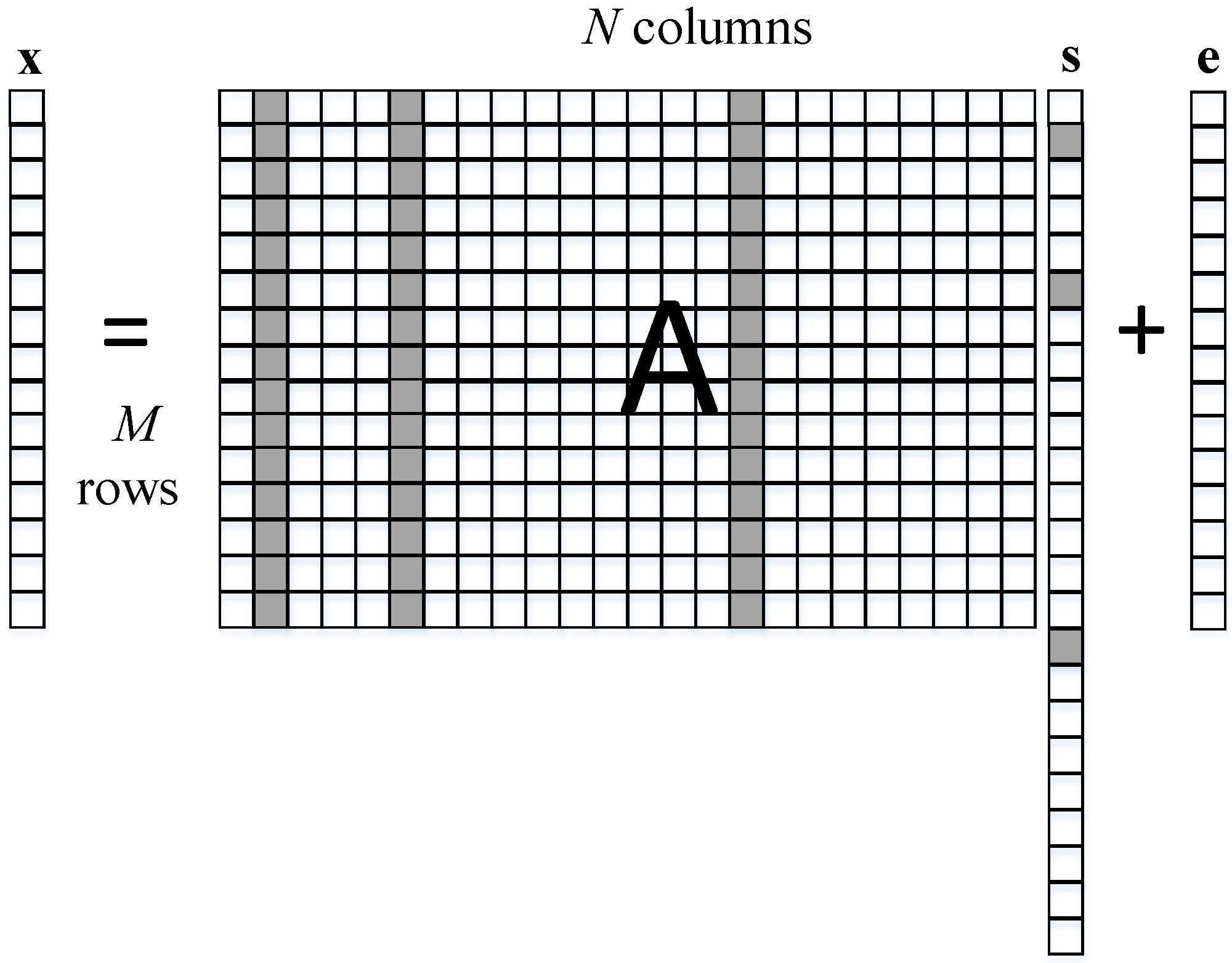
In this section we describe a novel and effective proposal for the constrained minimization problem in Equation (3). With complex noise and more sparsity, a challenging optimization problem has to be solved. The proposed algorithm is based on the signal model in Equation (1) presented in Figure 1, where is sparse enough so that the non-zero components, , in is less than . For the model, the measurement matrix and measurement vector are known, while the vector is to be estimated and reconstructed, under the assumption that is -sparse. denotes the estimated sparse vector.
For quantizing the fidelity of the estimation, one can measure a kind of distance between and . In the most situations, the root of mean square error is used usually for such purpose. If the error is Gaussian distributed, MSE is optimal, since the first and second moments incorporate all statistical characteristics. However, if the error is not Gaussian distributed, such as audio signal, image, communication signal, MSE will not be optimal. Considering the application to such cases, in this paper, we use the non-Gaussianity of error. As a sparse measure we use -norm. Therefore, the sparse vector can be estimated by minimizing the following objective function and formulate the optimization problem as follows
where denotes the negentropy, is -norm and is the regularizing parameter. Note that, algorithms based on MSE criterion have also proven to be weaker in the performances of convergence and accuracy.
Here, we apply the negentropy and -norm to construct the objective function, where the measurement of is negentropy and the sparsity constraint is for sparse-promoting. The small error on the zero components can be tolerated in exchange for high accuracy of the non-zero components in order to retain all significantly large components, so can be more exact and the performance of sparse signal reconstruction can be observably improved.
2.3 Algorithm
2.3.1. Negentropy Maximization
In the information theory, Gaussian variables have maximum entropy in all random variables which have the same variance. Therefore, one can use entropy to measure non-Gaussian noise. A modified form of entropy is negentropy which is used as the error measurement in the proposed algorithm. Negentropy can tolerate non-Gaussian noise on the signal so that the estimation of sparse signal becomes more accurate. The negentropy is defined as , where is the differential entropy and , is the Gaussian random variable which has the same variance with . When is Gaussian, . gets larger while becomes more non-Gaussian. reflects the non-Gaussian level of . When we apply the negentropy to the sparse signal reconstruction, the probability density distribution of variables is considered to be known. It is unpractical for the noise . Here, approximately, the negentropy is given by . Assume is super-Gaussian, which is non-Gaussian and the kurtosis value is greater than zero. This is true in most realistic situations, we can just use:
where denotes the statistical expectation. is the nonlinear function, such as , and [22]. In this paper, as an instance, the function is as follows:
where is constant. This nonlinear function is smooth and differentiable. When , is approximately equal to . Then, the gradient of can be calculated in order to maximize the negentropy so that can be minimized. It is an effective method to solve the optimization problem. The gradient of is calculated as:
where is the derivative of and .
The sparse signal can be iteratively updated as follows:
where represents the number of iterations and is the step size.
2.3.2. Weighted -norm and FOBOS
Considering the regulation, we find a sparse solution in the neighborhood of . That is we solve the problem as follows:
where is the updated vector from (9). Based on the understanding that the sparsity constraint resulting in sparser results when is closer to zero, we tend to choose value of between 0 and 1. However, this choice makes the optimization problem a concave one. To reform a convex sparsity constraint, we propose to approximate the -norm sparsity constraint with a weighted -norm. Thus, Equation (10) is rewritten as follows:
where is weight. Since and is close to 0, . Then, we update each component of by a FOBOS-like algorithm as:
where denotes the component of . When , .
To summarize, the method proposed in this paper is presented in Algorithm 1.
| Algorithm 1: Proposed algorithm for sparse signal reconstruction with negentropy and weighted -norm |
| Task: Estimate the sparse signal by minimizing Initialization: input signal matrix , system noise and proper and . Initialize and . Main iteration:
|
The stop condition can be the desired accuracy, convergence or a maximal iteration number.
3. Results and Discussions
In this section, we analyze the performance of the proposed algorithm for sparse signal reconstruction with negentropy and weighted -norm described in Section 2. In order to perform the numerical analysis, we present our experiment results to show whether the algorithm can recover the true sparse signal or not. The original sparse signal was sized as a 100 × 1 vector and generated by drawing value randomly from a normal distribution . In each sparse vector, there were several non-zero values, which were also picked and located randomly. The measurement matrix was sized as 40 × 100. Correspondingly, had 40 sample size and was generated by and using the equation . The noise vectors were added based on Gaussian and non-Gaussian random entries with various signal to noise ratios (SNR). The other parameters were set as below, . In order to evaluate the performance of the proposed algorithm, we use the normalized -error as a criteria to measure reconstruction accuracy for sparse signals, where the normalized -error is defined as .
3.1. The Reconstructed Signal Comparison between MSE Criterion and Proposed Algorithms
As discussed in Section 2.1, in the algorithm based on the MSE criterion, the objective function is:
The measurement of in Equation (13) is a Frobenius norm which is the common model of error [26]. As described in Section 2, we apply the negentropy and weighted -norm to form the objective function, where the measurement of is negentropy and the sparsity constraint can result in sparser results. Here, we compare the proposed algorithm with the MSE algorithm from the recovery and original signals images.
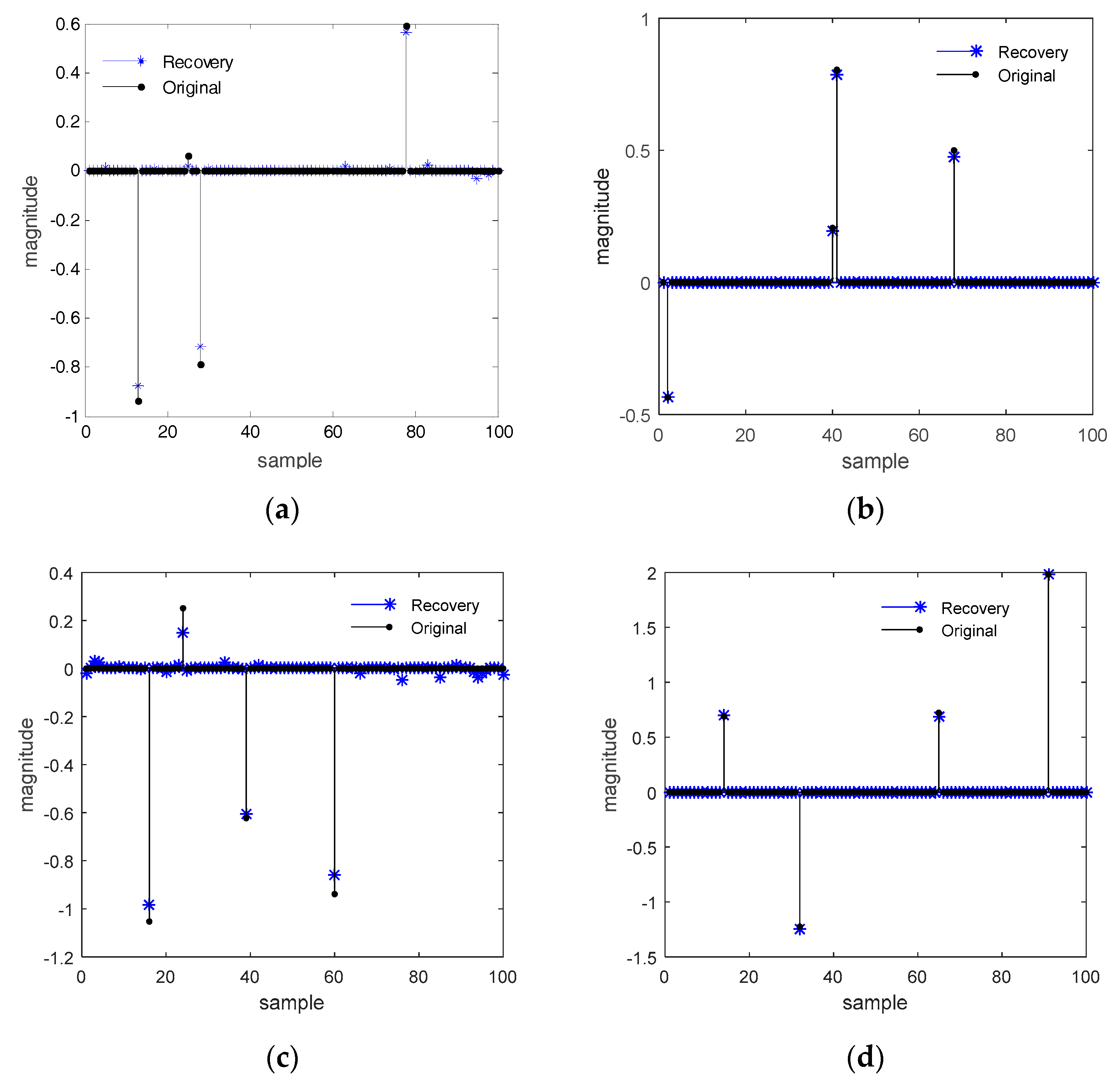
Figure 2 shows the reconstructed and original signal comparison between MSE and proposed algorithm. From Figure 2, it is clearly that MSE algorithm does not work well since it does not exploit the sparsity availably and is based on the assumption that noise has Gaussian characteristic. The zero components of is estimated exactly with the proposed algorithm, but is partly not zero with MSE algorithm. Furthermore, the non-zero components of is recovered more precisely with the proposed algorithm, where has better sparse characteristics.
3.2. The Accuracy Performance Comparison of the Algorithms
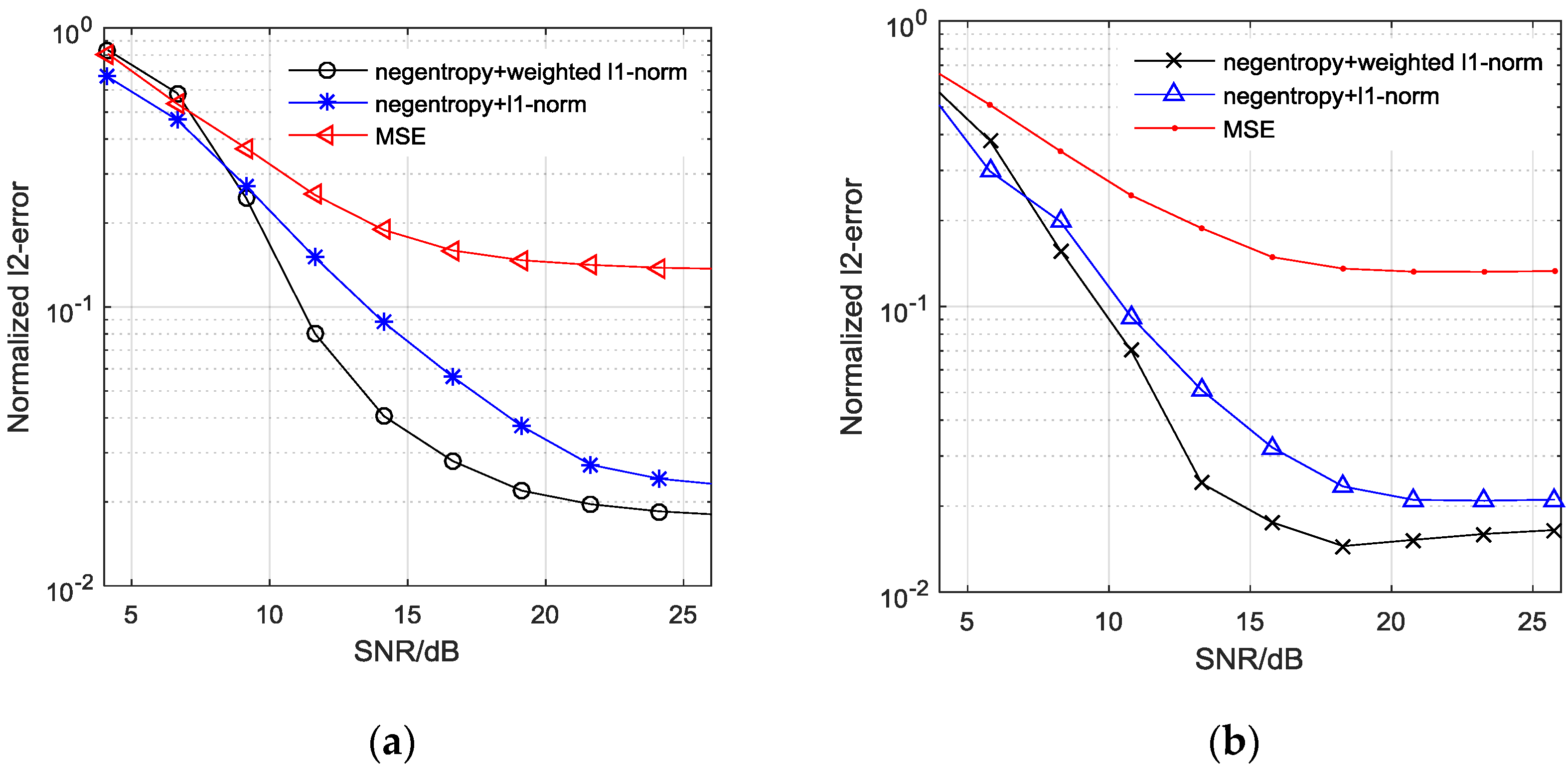
For a more complete description on how the performance is affected by noise, the normalized -error of is plotted under different SNR in Figure 3. The results demonstrate the significant reduction of normalized -error as SNR is increased. More specifically, the proposed algorithm has better performance that is at 10−2 order, compared with the MSE algorithm that is at 10−1 order. Therefore, the proposed algorithm has higher accuracy as expected and is more suitable for sparse signal reconstruction with complex noise.
3.3. The Convergence Performance Comparison of the Algorithms
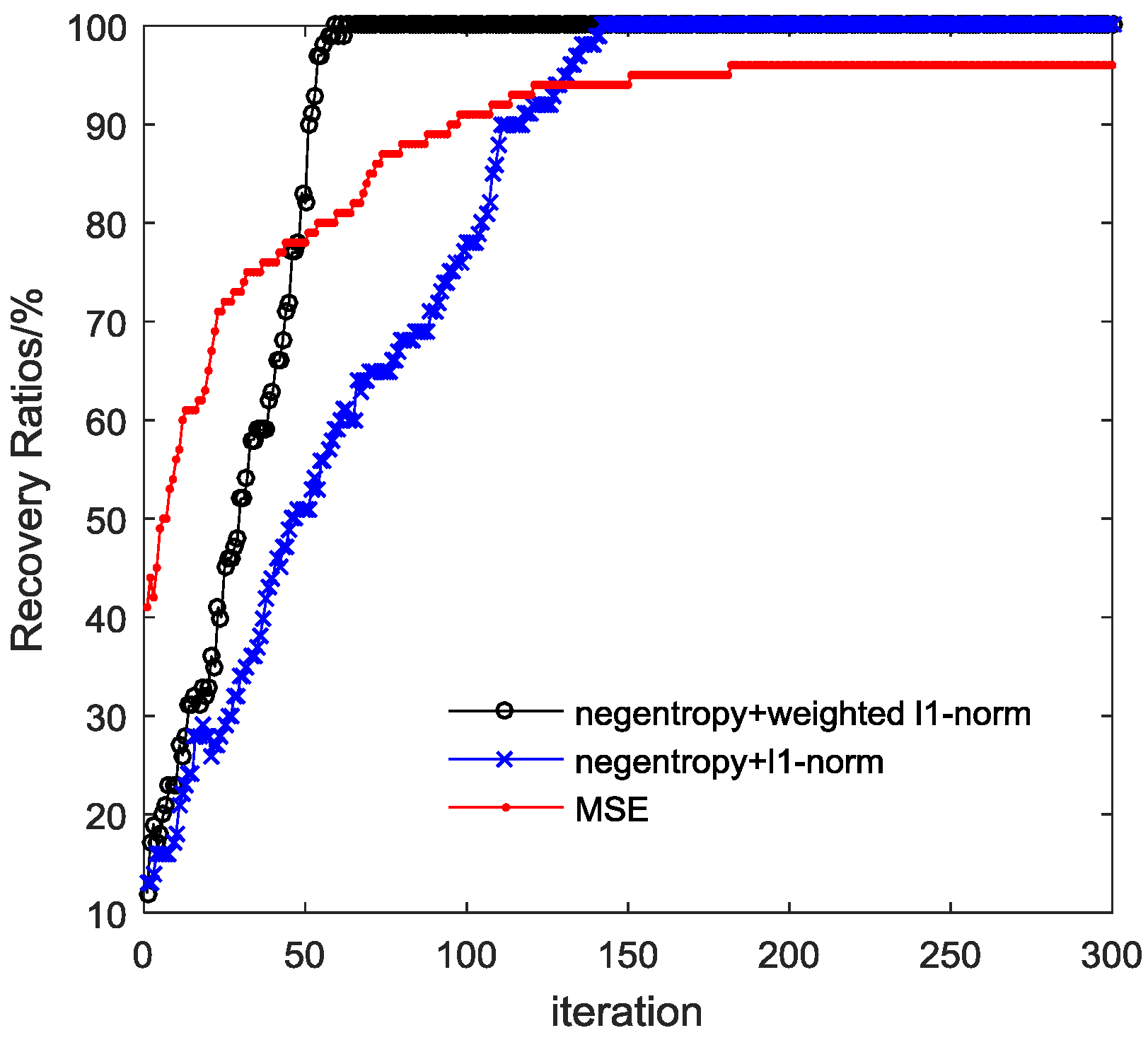
To illustrate the convergence of the algorithm, we present the performance of normalized -error with the iterations in Figure 4 in the same non-Gaussian noise circumstance. As the number of iterations increases, the relative error of reconstructed sparse signal decreases, and becomes stable at a certain error value where the convergence is reached. Figure 4 shows that the number of iterations for convergence of the proposed algorithm is smaller than that of MSE. It can be seen that the proposed algorithm converged faster. Novel loss function and FOBOS-like algorithm lead to the better performance in convergence rate. Besides, the stable normalized -error is lower compared to that of MSE seen in Figure 4. With respect to the performance of reconstructing sparse signals, the recovery ratios are shown in Figure 5. The recovery ratio of the proposed algorithm can reach 100% with the smaller number of iterations than that of MSE. Therefore, the proposed algorithm has significant advantages in computational complexity and specially in recovery ratio.
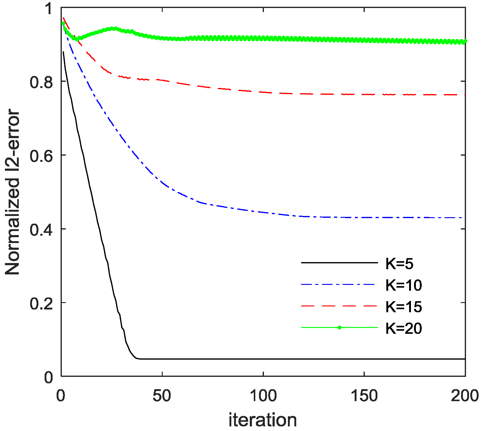
Figure 6 presents the normalized -error with the sparsity level which is the number of non-zero components in all components. We consider a randomly generated -sparse signal of length and non-zero components. It is apparent that for different sparse signals, the normalized -error is reduced through decreasing the number of non-zero components. Therefore, when implementing the proposed strategy in practice, it is important to consider the sparsity of signals.
4. Conclusions
We have presented an effective algorithm for reconstructing sparse signals, which is based on a convex optimization problem upon the proposed objective function. The objective function includes the negentropy as the fitting error measurement and -norm, which is treated as the weighted -norm, as the sparse-promotion. Furthermore, the proposed algorithm includes two main steps in each iteration: (1) gradient based maximization to the negentroy; (2) a soft thresholding to the result of (1), for sparsity promotion. Experiments show that the proposed algorithm has improved accuracy and convergence rate, especially when the noise is non-Gaussian in the information transmission. In our future research, the algorithm will be optimized for complexity and the real-world applications in signal processing and communication fields will also be considered.
Acknowledgments
This work is supported by the National Natural Science Foundation of China under grant nos. 61501262 and 61571244, by Tianjin Research Program of Application Foundation and Advanced Technology under grant nos. 15JCYBJC51600 and 16YFZCSF00540.
Author Contributions
Yingxin Zhao and Zhiyang Liu conceived and designed thealgorithm; Yuanyuan Wang performed thesimulation; Yingxin Zhao and Shuxue Ding analyzed theresults; Hong Wu contributed the simulation tools; Yingxin Zhao and Shuxue Ding wrote and revised the paper.
Conflicts of Interest
The authors declare no conflict of interest.
References
- Elad, M.; Figueiredo, M.; Ma, Y. On the role of sparse and redundant representations in image processing. Proc. IEEE 2010, 98, 972–982. [Google Scholar] [CrossRef]
- Li, B.; Du, R.; Kang, W.J.; Liu, G.L. Multi-user detection for sporadic IDMA transmission based on compressed sensing. Entropy 2017, 19, 334. [Google Scholar]
- Shi, W.T.; Huang, J.G.; Zhang, Q.F.; Zheng, J.M. DOA estimation in monostatic MIMO array based on sparse signal reconstruction. In Proceedings of the IEEE International Conference on Signal Processing, Communications and Computing, Hong Kong, China, 5–8 August 2016; pp. 1–5. [Google Scholar]
- Chen, Y.; Gu, Y.; Hero, A.O. Sparse LMS for system identification. In Proceedings of the IEEE International Conference on Acoustics, Speech and Signal Processing, Taipei, Taiwan, 19–24 April 2009; pp. 3125–3128. [Google Scholar]
- Singer, A.C.; Nelson, J.K.; Kozat, S.S. Signal processing for underwater acoustic communications. IEEE Commun. Mag. 2009, 47, 90–96. [Google Scholar] [CrossRef]
- Yousef, N.R.; Sayed, A.H.; Khajehnouri, N. Detection of fading overlapping multipath components. Signal Process. 2006, 86, 2407–2425. [Google Scholar] [CrossRef]
- Donoho, D.L. Compressed sensing. IEEE Trans. Inf. Theory 2006, 52, 1289–1306. [Google Scholar] [CrossRef]
- Candes, E.J.; Romberg, J.; Tao, T. Robust uncertainty principles: Exact signal reconstruction from highly incomplete frequency information. IEEE Trans. Inf. Theory 2004, 52, 489–509. [Google Scholar] [CrossRef]
- Xu, W.; Lin, J.; Niu, K.; He, Z. A joint recovery algorithm for distributed compressed sensing. IEEE Trans. Emerg. Telecommun. Technol. 2012, 23, 550–559. [Google Scholar] [CrossRef]
- Figueiredo, M.; Nowak, R.S.; Wright, S.J. Gradient projection for sparse reconstruction: Application to compressed sensing and other inverse problems. IEEE J. Sel. Top. Signal Process. 2007, 1, 586–598. [Google Scholar] [CrossRef]
- Kim, S.; Koh, K.; Lustig, M.; Boyd, S.; Gorinvesky, D. An interior point method for large-scale l1-regularized least squares. IEEE J. Sel. Top. Signal Process. 2007, 1, 606–617. [Google Scholar] [CrossRef]
- Bioucas-Dias, J.; Figueiredo, M. A new TwIST: Two step iterative shrinkage-thresholding algorithms for image restoration. IEEE Trans. Image Process. 2007, 16, 2992–3004. [Google Scholar] [CrossRef] [PubMed]
- Bredies, K.; Lorenz, D.A. Iterated hard shrinkage for minimization problems with sparsity constraints. SIAM J. Sci. Comput. 2008, 30, 657–683. [Google Scholar] [CrossRef]
- Montefusco, L.B.; Lazzaro, D.; Papi, S. A fast algorithm for nonconvex approaches to sparse recovery problems. Signal Process. 2013, 93, 2636–2647. [Google Scholar] [CrossRef]
- Montefusco, L.; Lazzaro, D.; Papi, S. Fast sparse image reconstruction using adaptive nonlinear filtering. IEEE Trans. Image Process. 2011, 20, 534–544. [Google Scholar] [CrossRef] [PubMed]
- Leung, S.H.; So, C.F. Gradient-based variable forgetting factor RLS algorithm in time-varying environments. IEEE Trans. Signal Process. 2005, 53, 3141–3150. [Google Scholar] [CrossRef]
- Eksioglu, E.M. RLS algorithm with convex regularization. IEEE Signal Process. Lett. 2011, 18, 470–473. [Google Scholar] [CrossRef]
- Liu, J.M.; Grant, S.L. Proportionate Adaptive Filtering for Block-Sparse System Identification. IEEE Trans. Audio Speech Lang. Process. 2016, 24, 623–630. [Google Scholar] [CrossRef]
- Zhang, Y.W.; Xiao, S.; Huang, D.F.; Sun, D.J.; Liu, L.; Cui, H.Y. l0-norm penalised shrinkage linear and widely linear LMS algorithms for sparse system identification. IET Signal Process. 2017, 11, 86–94. [Google Scholar] [CrossRef]
- Wu, F.Y.; Tong, F. Non-Uniform Norm Constraint LMS Algorithm for Sparse System Identification. IEEE Commun. Lett. 2013, 17, 385–388. [Google Scholar] [CrossRef]
- Magill, D. Adaptive minmum MSE estimation. IEEE Trans. Inf. Theory 1963, 9, 289. [Google Scholar] [CrossRef]
- Woodward, P. Entropy and negentropy. IRE Trans. Inf. Theory 1957, 3, 3. [Google Scholar] [CrossRef]
- Yamamoto, T.; Yamagishi, M.; Yamada, I. Adaptive Proximal Forward-Backward Splitting for sparse system identification under impulsive noise. In Proceedings of the 20th European Signal Processing Conference, Bucharest, Romania, 27–31 August 2012; pp. 2620–2624. [Google Scholar]
- Theodoridis, S.; Kopsinis, Y.; Slavakis, K. Sparsity-Aware Learning and Compressed Sensing: An Overview. Inf. Theory 2012, 11, 7–12. [Google Scholar]
- Stefan, V.; Isidora, S.; Milos, D.; Ljubisa, S. Comparison of a gradient-based and LASSO algorithm for sparse signal reconstruction. In Proceedings of the 5th Mediterranean Conference on Embedded Computing, Bar, Montenegro, 12–16 June 2016; pp. 377–380. [Google Scholar]
- Su, G.; Jin, J.; Gu, Y.; Wang, J. Performance analysis of l0-norm constraint least mean square algorithm. IEEE Trans. Signal Process. 2012, 60, 2223–2235. [Google Scholar] [CrossRef]
Figure 1.
Signal model with .

Figure 2.
Reconstructed signal and original signal comparison between MSE and proposed algorithms. (a) MSE algorithm with Gaussian noise; (b) proposed algorithm with Gaussian noise; (c) MSE algorithm with non-Gaussian noise; (d) proposed algorithm with non-Gaussian noise.
Figure 2.
Reconstructed signal and original signal comparison between MSE and proposed algorithms. (a) MSE algorithm with Gaussian noise; (b) proposed algorithm with Gaussian noise; (c) MSE algorithm with non-Gaussian noise; (d) proposed algorithm with non-Gaussian noise.

Figure 3.
Normalized -error performance versus SNR. (a) comparison between MSE and proposed algorithms with Gaussian noise; (b) comparison between MSE and proposed algorithms with non-Gaussian noise.
Figure 3.
Normalized -error performance versus SNR. (a) comparison between MSE and proposed algorithms with Gaussian noise; (b) comparison between MSE and proposed algorithms with non-Gaussian noise.

Figure 4.
Normalized -error performance versus iteration number.
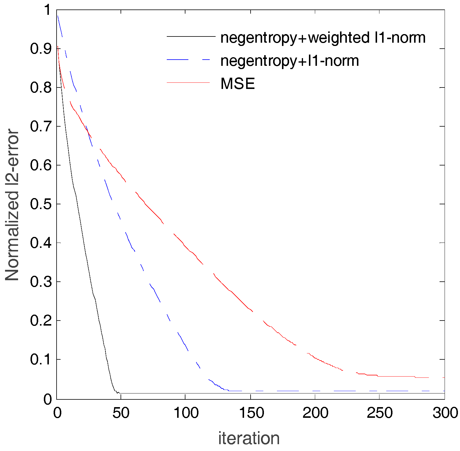
Figure 5.
Recovery ratios of versus iteration number.

Figure 6.
Normalized -error performance versus iteration number for different sparse signal with the proposed algorithm.
Figure 6.
Normalized -error performance versus iteration number for different sparse signal with the proposed algorithm.

© 2017 by the authors. Licensee MDPI, Basel, Switzerland. This article is an open access article distributed under the terms and conditions of the Creative Commons Attribution (CC BY) license (http://creativecommons.org/licenses/by/4.0/).
Share and Cite
MDPI and ACS Style
Zhao, Y.; Liu, Z.; Wang, Y.; Wu, H.; Ding, S. Sparse Coding Algorithm with Negentropy and Weighted ℓ1-Norm for Signal Reconstruction. Entropy 2017, 19, 599. https://doi.org/10.3390/e19110599
AMA Style
Zhao Y, Liu Z, Wang Y, Wu H, Ding S. Sparse Coding Algorithm with Negentropy and Weighted ℓ1-Norm for Signal Reconstruction. Entropy. 2017; 19(11):599. https://doi.org/10.3390/e19110599
Chicago/Turabian StyleZhao, Yingxin, Zhiyang Liu, Yuanyuan Wang, Hong Wu, and Shuxue Ding. 2017. "Sparse Coding Algorithm with Negentropy and Weighted ℓ1-Norm for Signal Reconstruction" Entropy 19, no. 11: 599. https://doi.org/10.3390/e19110599
Note that from the first issue of 2016, this journal uses article numbers instead of page numbers. See further details here.