Partial and Entropic Information Decompositions of a Neuronal Modulatory Interaction


1
Department of Statistics, University of Glasgow, Glasgow G12 8QQ, UK
2
Institute of Neuroscience and Psychology, University of Glasgow, Glasgow G12 8QQ, UK
3
Faculty of Natural Sciences, University of Stirling, Stirling FK9 4LA, UK
*
Author to whom correspondence should be addressed.
Entropy 2017, 19(11), 560; https://doi.org/10.3390/e19110560
Submission received: 30 June 2017
/
Revised: 27 September 2017
/
Accepted: 23 October 2017
/
Published: 26 October 2017
(This article belongs to the Special Issue Information Decomposition of Target Effects from Multi-Source Interactions)
Abstract
:Information processing within neural systems often depends upon selective amplification of relevant signals and suppression of irrelevant signals. This has been shown many times by studies of contextual effects but there is as yet no consensus on how to interpret such studies. Some researchers interpret the effects of context as contributing to the selective receptive field (RF) input about which neurons transmit information. Others interpret context effects as affecting transmission of information about RF input without becoming part of the RF information transmitted. Here we use partial information decomposition (PID) and entropic information decomposition (EID) to study the properties of a form of modulation previously used in neurobiologically plausible neural nets. PID shows that this form of modulation can affect transmission of information in the RF input without the binary output transmitting any information unique to the modulator. EID produces similar decompositions, except that information unique to the modulator and the mechanistic shared component can be negative when modulating and modulated signals are correlated. Synergistic and source shared components were never negative in the conditions studied. Thus, both PID and EID show that modulatory inputs to a local processor can affect the transmission of information from other inputs. Contrary to what was previously assumed, this transmission can occur without the modulatory inputs becoming part of the information transmitted, as shown by the use of PID with the model we consider. Decompositions of psychophysical data from a visual contrast detection task with surrounding context suggest that a similar form of modulation may also occur in real neural systems.
1. Introduction
Amplifiers, such as hearing aids, for example, are designed to increase signal strength without distorting the informative content that it transmits, i.e., its “semantics”. Though independence of semantics has been a truism of information theory since its inception, information decomposition may help distinguish the effects of amplifying inputs from driving inputs which determine what the output transmits information about, which is what we will refer to here as its “semantics”. It may seem intuitively obvious that any output must necessarily transmit information about all inputs that affect it, but that intuition is misleading. Here, we use information decomposition to show that a modulatory input can influence the transmission of information about other inputs while remaining distinct from that information.
This may help resolve a long-standing controversy within the cognitive neurosciences concerning the nature of “contextual modulation”. Many see the wide variety of psychophysical and physiological phenomena that are grouped under this heading as demonstrating that the concept of a neuron’s receptive field, i.e., what the cell transmits information about, needs to be extended to include an extra-classical receptive field; see e.g., [1]. In contrast to that many others see these phenomena as evidence that contextual modulation does not change the cell’s receptive field semantics; see e.g., [2,3,4].
Resolution of this issue requires an adequate definition of “modulation”, which is used in several different, and often undefined, ways. It is frequently used to mean simply that one thing affects another. That unnecessary use of the term introduces substantial confusion, however, because the term is also often used to refer to a three-term interaction. It could be used to refer to any three-way interaction in which A effects the transmission of information about B by C. Our use is more specific than that, however. The essence of the modulatory interaction that we study here is that the modulator affects transmission of information about something else without becoming part of the information transmitted. The effect of the volume control on a radio provides a simple example. It changes signal strength without becoming part of the message conveyed. The use of the term “modulation” in telecommunications potentially adds further confusion, however, because in either amplitude modulation (AM) or frequency modulation (FM) it is the “modulatory” signal that is used to convey the message to be transmitted. That is the opposite of what we and many others in the cognitive and neurosciences refer to as “modulation”. While awaiting a consensus that resolves this terminological confusion we define our usage of the term “modulation” as explicitly and as clearly as we can. Modulation that increases output signal strength is referred to as “amplification” or “facilitation”. Modulation that decreases output signal strength is referred to as “disamplification”, “suppression”, or “attenuation”.
Information decomposition could help clarify the notion of “modulation” as used within the cognitive and neurosciences in at least three ways. First, by requiring formal specifications to which decompositions can be applied it enforces adequate definition. Second, by being applied to a transfer function explicitly designed to be modulatory, it deepens our understanding of the information processing operations performed by such interactions. Third, decomposition of a modulatory interaction that is formally specified shows the conditions under which it can be distinguished from additive interactions and provides patterns of decomposition to which empirically observed patterns can be compared.
In this paper we apply information decomposition to a transfer function specifically designed to operate as a modulator within a formal neural network that uses contextually guided learning to discover latent statistical structure within its inputs [5]. We show that this transfer function has the properties required of a modulator, and that they can be clearly distinguished from additive interactions that do contribute to output semantics. A thorough understanding of this modulatory transfer function is of growing importance to neuroscience because recent advances suggest that something similar occurs at an intracellular level in neocortical pyramidal cells, and may be closely related to consciousness [6,7]. It is also important to machine learning because the information processing capabilities of networks such as those used for deep learning might be greatly enhanced if given the context-sensitivity that such modulatory interactions can provide.
Modulatory interactions distinguish the contributions of two distinct inputs to an output, so they imply some form of multivariate mutual information decomposition. Various forms of decomposition have been proposed, however, and they may offer different resolutions to this issue. We therefore compare resolutions that arise from two proposals discussed elsewhere in this Special Issue. One is Partial Information Decomposition [8,9,10,11]. The other is Entropic Information Decomposition [12,13]. We find that though there are important differences between these two proposed forms of decomposition, they are in agreement with respect to their implications for the issue of distinguishing between additive and modulatory interactions.
The notion of modulation is essentially a three-term interaction in which one input variable modulates transmission of information about a second input variable by an output. The two inputs therefore make fundamentally different kinds of contribution to the output. In contrast to that, additive interactions do not require the two inputs to remain distinct because their contributions can be summarized via a single integrated value. Many information decomposition spectra and surfaces are displayed in the following, demonstrating their expressive power and the variety of information processing operations that a single transfer function can perform.
2. Notation and Definitions
In this section we describe our notation and define the information-theoretic concepts which are used in the sequel. A generic “p” is used to denote a probability mass function, with the argument of the function signifying which distribution is being described. Capital letters are used to denote random variables, with their realised values appearing in lower-case. We denote the conditional probability that , given that and by the conditional mass function for and , where .
In [14], the RF and contextual field (CF) inputs were multivariate, but here we consider the special case of the local processor in [14] having two binary inputs, and , and one binary output, Y, with all three random variables having range space B. The joint distribution of is given by the probability mass function (p.m.f.) where
This distribution will be considered in the form
and we will separately specify a joint p.m.f and a conditional p.m.f. .
In the local processor in Figure 1, the value of provides the receptive field (RF) input to the local processor, while the value of is the input from the contextual field (CF). The value of the RF input, , is multiplied by the signal strength to form the integrated RF input and similarly for the CF input, . Therefore, the values taken by the integrated RF and CF inputs are and These integrated values have both strength and a sign. The strength is a constant property of the defined system, while the sign can change from sample to sample. The signal strengths, , are positive real numbers. The manner in which these signals are combined in the output unit will be described in Section 3.
In this study, it is assumed that and that the correlation between and is d, where . This means that
It is also assumed that the conditional output probability has a logistic form, with
where T is a transfer function which depends also on the signal strengths, In Section 3, the two transfer functions that are used in this study are specified. It should be noted that we are actually considering a class of trivariate probability distributions that are indexed by where although this indexation is suppressed in the sequel for ease of notation. The various classical measures of information and measures of partial information used are calculated using a member of the class of trivariate probability distributions, defined in (1)–(4), that is given by a particular choice of
We now define the standard information theoretic terms that are required in this work and based on results in [15]. We denote by the function H the usual Shannon entropy, and note that any term with zero probabilities makes no contribution to the sums involved. The total mutual information that is shared by Y and the pair is given by,
The information that is shared between Y and but not with is
and the information that is shared between Y and but not with is
Finally, the co-information of has several equivalent forms
where, for ,
We note that classical Shannon information measures have been used in neural coding studies to investigate measures of synergy and redundancy; see for example [16].
When we come to define measures of partial information it will be necessary to calculate these information quantities with respect to another p.m.f., say , and to denote this we add the subscript “q” to such terms, e.g., This means that the p.m.f. is used in the computation rather than the original p.m.f.
3. An Interaction Designed to Be Modulatory
Our concern here is with variables that can take either positive or negative values, which can be seen as being analogous to excitation and inhibition in neural systems. We model that decision as a probabilistic binary variable that chooses between the values 1 and −1. The criteria to be met by a modulatory transfer function in this case have been stated and discussed in many previous papers; see e.g., [17,18,19]. The criteria for a modulatory interaction were stated for a local processor receiving two inputs: the integrated RF input, r, and the integrated CF input, c. The requirements were stated in terms of the level of activation within the local processor, although in this paper we use this term to denote the value of the transfer function, and they are amended slightly here. Please note that the term ’integrated’ was used in previous work to refer to the weighting and summing of the components of a multivariate input; we continue to use this term here even though the input to each field is univariate. The value of the transfer function is fed into a logistic function to compute the conditional probability that a 1 will be transmitted. Stated in those terms the CF input modulates transmission of information about the RF input if four criteria are met:
- If the integrated RF input is extremely weak, then the value of the transfer function is close to zero.
- If the integrated CF input is extremely weak, then the value of the transfer function should be close to the integrated RF input.
- If the integrated RF and CF inputs have the same sign, then the absolute value of the transfer function should be greater than when based on the RF input alone. On the other hand, if the RF and CF inputs are of opposite sign then the absolute value of the transfer function should be less than when based on the RF input alone.
- The sign of the value of the transfer function is that of the integrated RF, so that the context cannot change the sign of the conditional mean of the output.
In general terms, the CF input would have no modulatory effect on the output when the output and the CF input are conditionally independent given the value of the RF input, which is equivalent to the conditional mutual information being equal to zero. One case where this happens for any member of the class of trivariate binary distributions defined in (1)–(4) is when the correlation between the inputs is , for then see Theorem 5. On the other hand, in situations where this conditional mutual information is non-zero then influences the prediction of the output Y by the input in the sense that
for at least one This is a very general form of modulation, but the type of modulation defined in requirements 1–4 is very specific and we call it “contextual modulation”. This contextual modulation is relevant within the local processor at the level of individual system inputs and outputs. On the other hand, the following conditions express the notion of contextual modulation for the whole ensemble of inputs and outputs:
- M1:
- If the signal is strong enough and the CF input is extremely weak then can have its maximum value, can be maximised and is close to zero. This shows that the RF input is sufficient, thus allowing the information in the to be transmitted, and that the CF input is not necessary.
- M2:
- and are close to zero when the RF input is extremely weak no matter how strong the CF input. This shows that the RF input is necessary for information to be transmitted, and that the CF input is not sufficient to transmit the information in the RF input.
- M3:
- When and when the RF input is weak, and are both larger when the CF input is moderate than when the CF input is weak. Thus the CF input modulates the transmission of information about the RF input.
One might expect that these two definitions of contextual modulation are linked. In the limiting situation of it is possible to show that requirement 1 implies M1, and as one finds that requirement 2 implies M2. It seems difficult to prove more general connections and so this matter is considered computationally in Section 3.1.
Multivariate binary processors were also considered in [5], thus allowing for choice between many more than two alternatives. It was also shown that the coherent infomax learning rule also applies to this multivariate case such that the contextually guided learning discovers variables defined on the RF input space that are statistically related to variables specified in, or discovered by, other streams of processing within the network. Thus it implements a multi-stream, non-linear, form of latent structure analysis. There are two distinct aspects of semantics in this system, i.e., the receptive field selectivity of each unit within a local processor and the positivity or negativity of its output. Here we are primarily concerned with that latter aspect. We show below that:
- (i)
- the modulatory input affects output only when the primary driving integrated RF input is non-zero but weak;
- (ii)
- that even when it does have an effect it has no effect on the sign of the conditional mean output, and
- (iii)
- that it can have those modulatory effects without the binary output transmitting any unique information about the modulator.
In the case where the processor has a binary output, the transfer function has the form
where , and are constants, and here we take and .
This transfer function was designed to effect a modulatory interaction between two input sources, with one source being the primary driver while the role of the the second “contextual” source is to modulate transmission of information about the primary source. The effect of the contextual source is to amplify or disamplify the strength of the signal from the primary source in such a way that the semantic content (the sign) of the primary source is not changed. Neither of the PID and EID considered in this paper has previously been applied to this kind of signal and we now show this to be possible.
In this paper, the version of the modulatory transfer function we use takes the form
for given values of the random variables and given signal strengths . Here the integrated RF input is and the integrated CF input is and they both have a sign and a strength. The output conditional probability is given by
Whether this probability is greater than or less than is determined solely by the value of , and the form of ensures that the contextual signal cannot change the sign of the output conditional mean. Thus the output produced has semantic content, and also the value of the output conditional probability, , gives the semantic content a measure of strength in the sense that values of closer to 0 or 1 indicate a more definite decision. The conditional variance of Y is , and so uncertainty in the output decision is largest when and zero when or 1. An alternative description is to say that the precision (reciprocal variance) is least when and it tends to infinity as approaches 0 or 1. Within the local processor the conditional mean of the output, , is also computed. It has both a sign and a strength.
Given the form of , the integrated RF will be amplified in magnitude whenever the signs of and agree, and it will be disamplified when these signs do not agree. The role of the integrated CF is to modify the strength of the conditional mean output without conveying its own semantic content (i.e., its sign). This form of transfer function ensures that the maximum extent of any disamplification of the primary signal is by a factor of 2.
By way of contrast, we also consider an additive transfer function by simply adding together the integrated RF and CF inputs, , to give
with the output conditional probability given by
The use of this transfer function also affects the values of and m but, unlike the modulatory transfer function, this additive transfer function can change the sign of the output conditional mean m, which is not consistent with the fourth condition for a modulatory transfer function described above. The additive transfer function does satisfy condition M1 but does not satisfy condition M2 or M3. This additive transfer function can be seen as a simple version of the common assumption within neurobiology that neurons function as integrate-and-fire point processors. While this assumption does not imply that all integration is linear it does mean that such integration computes a single value per local processor. The results produced using the these two different transfer functions will be discussed in Section 5, Section 6, Section 7 and Section 8.
Please note that in the sequel we normally abbreviate the terms “integrated RF input” and “integrated CF input” by using just “RF input” and “CF input”, respectively. In particular, whenever a strength is implied for the RF or CF input, then we mean that the ‘integrated’ values of these inputs are being considered.
3.1. Analysis Using Classical Shannon Measures
We start in this section by presenting results involving the classical Shannon measures for the system defined in Section 2 and Section 3. First we recall that and are defined in (2) and (3) and set up some further simplifying notation which is used in the results. We set
The parameters u and v are function of and , and u takes the value or depending on which transfer function is being used; similarly for v. From (10) for transfer function
whereas, from (12), for transfer function
Finally, we define
where We note also that the value of z has two forms: when transfer function is used and when transfer function is employed; similarly for w. We now collect together our results in the following theorem, proof of which is relegated to the appendix.
Theorem 1.
- (a)
- (b)
- (c)
- (d)
- (e)
- (f)
Since we are particularly interested in interactions among the three variables, we now show the classic Shannon information measures defined in (6)–(9), with surface plots given in Figure 2 and Figure 3. A correlation between the inputs of was considered to ensure that these measures have the same maximum possible value of bits, and a zero correlation was considered to represent the case of independent inputs. One purpose is to discuss the general links between requirements 1–4 and conditions M1–M3 from Section 3 and also the use of the transfer functions defined in (10) and (12).
First, we notice in Figure 2 that the modulatory and additive transfer functions produce very different surfaces. In Figure 2a,b, the surface for rises more quickly to its maximum than the surface for and in Figure 2a sections parallel to the axis are similar for whereas the surface for is symmetric about the line . Figure 2d,f,h,j and Figure 3d,f,h,j for show clear asymmetry about the line
When the strength of the CF input, , is very small we notice in Figure 2e and Figure 3e that is close to zero. Figure 2c shows that rises quickly, then gradually, towards its maximum at 0.5 as the strength of the RF input, , increases, as does the surface in Figure 3c although there the maximum value is higher at 1. Figure 2g and Figure 3g show that rises towards a maximum value of 1; this rise is much steeper when the correlation is 0.78 than when it is zero. These observations provide support for condition M1 when the modulatory transfer function is used. Similar observations on the corresponding figures based on the use of the additive transfer function show that condition M1 is satisfied in this case also.
Figure 2e,g and Figure 3e,g show, when is close to zero, that and are both close to zero, thus supporting condition M2 when the modulatory transfer function is used. This is not the case when the additive transfer function is employed, as can be seen from Figure 2f,h and Figure 3f,h. It is important to note that these figures do not all use the same scales for the heights of the surface. For example, the scales of Figure 2e and Figure 3e are expanded because is always small when the transfer function is modulatory.
Also, when the strength of the RF input is weak (say ), we notice in Figure 2c,g and Figure 3c,g that both and are larger for moderate CF strengths (say ) than when the the strength of the CF input is extremely weak (, say), with this effect being stronger when the correlation between inputs is 0.78. This provides support for condition M3 when the modulatory transfer function is used. Inspection of the corresponding plots based on the additive transfer function show this effect only for in Figure 2h, and so condition M3 does not hold for the additive function.
In Figure 3a,b, the surfaces of the co-information are negative, as expected from (8), since the correlation between and is zero and so their mutual information is zero.
Finally we focus discussion on the phenomenon of particular relevance to the subject of this paper by considering the surface plots of In Figure 2e, an interesting pattern emerges. There is a steep rise for small values of and for all values of , and then the surface quickly dies away. This pattern is repeated in Figure 3e. This suggests that is affecting the information shared between Y and , indicating that modulation of some form might be taking place.
It could be argued, however, that is part of the output semantics in the sense that the output contains information specifically about itself. Since is clearly positive for these values of it is impossible to know whether or not this is the case based on this classical Shannon measure. It was shown in [8], that could be decomposed into two terms: the unique information that conveys about Y as well as synergistic information that is not available from alone, but rather gives the information that and , acting jointly, have about the output Y. We now apply information decompositions in order to resolve these different interpretations. For discussion of some limitations of classical Shannon measures and the need for new measures of information, see [20].
4. Information Decompositions
Williams and Beer [8] introduce a framework called the Partial Information Decomposition (PID) which decomposes mutual information between a target and a set of multiple predictor variables into a series of terms reflecting information which is shared, unique or synergistically available within and between subsets of predictors. Here we focus on the case of two input predictor variables, denoted , and an output target Y. The information decomposition can be expressed as
and it is the basis of both the information decompositions described in Section 4.1 and Section 4.2. Adapting the notation of [21] we express our joint input mutual information in four terms as follows:
| denotes the unique information that conveys about Y; | |
| is the unique information that conveys about Y; | |
| gives the common (or redundant or shared) information that both and have about Y; | |
| is the synergy or information that the joint variable has about Y that cannot be obtained by observing and separately. |
It is possible to make deductions about a PID by using the following four equations which give a link between the components of a PID and certain classical Shannon measures of mutual information. The following are from Equations (4) and (5) in [21], with amended notation; see also [8].
We will refer to these results in Section 5 and use them in Section 6.
We consider here two different information decompositions. Although there are clear conceptual differences between the two, where they agree we can have some confidence we are accurately decomposing information as we would like. Where they disagree, we hope this may shed light on particular properties of the modulatory systems we study here, and also provide interesting comparisons of the two approaches.
It has been noted [22] that there are two different ways shared information can emerge. Source shared information refers to shared information that arises simply because the two inputs are correlated. For example, if but and are correlated then there will be some and some redundancy , even though plays no role in the computation implemented by the local processor. However, redundancy can also occur in systems where the inputs are statistically independent—in this case, it is referred to as mechanistic shared information, since it arises as a property of the function of the local processor. We denote as the standard PID measure of shared information which quantifies both of these types together. However, both decompositions we consider provide a way to separately quantify these two types of shared information, which we denote by and for source and mechanistic respectively.
4.1. The Ibroja PID
In the Ibroja PID [9,10], the shared information component is based on an assumption that the information shared between two predictors about a target should not be affected by the marginal distribution of the two inputs when the output is ignored. Instead, the shared information is a function only of the individual input-output marginal distributions of and . In other words, the information about the output which is shared between the two inputs is independent of the correlation between the two inputs. In [9], this is motivated with an operational definition of unique information based on decision theory. It is claimed that unique information in input should correspond to the existence of a decision problem where two agents must try to guess the value of the output Y in which an agent acting optimally on evidence from can do systematically better (higher expected utility) than an agent acting optimally based on evidence from see also Appendix B2 in [21].
Following notation in [9], we consider a given joint distribution p for , we let be the set of all joint distributions of Y, and , and define
as the set of all joint distributions which have the same and marginal distributions as p.
In Lemma 4 in [9] five equivalent optimisation problems are defined involving various information components. In this work we chose to minimise the total mutual information in order to find the optimal distribution denoted by . For the description of EID in Section 4.2, we note that this is equivalent to finding the distribution in which maximizes the co-information . This optimal distribution is then used to calculate the four partial information measures:
and the information quantities, except , are calculated with respect to the optimal distribution
Using equations (7) & (8) from [23], the shared information can be split into non-negative source and mechanistic components that are defined as follows (in amended notation).
A particular advantage of the Ibroja approach is that it results in a decomposition consisting of non-negative terms. A possibly counter-intuitive feature is that in our two input, one output local processor context, one might expect that should change depending on the marginal distribution of the inputs, , in that source shared information should increase as the correlation between the inputs increases (assuming the individual input-output marginals are fixed). In the systems defined in Section 2, however, the marginal distributions of and do depend on the correlation between the inputs, and so the Ibroja PID does change as this correlation changes.
4.2. The EID Using
An alternative measure of shared information was recently proposed in [12]. Since at a local or pointwise level [24,25,26,27,28] (i.e., the terms inside the expectation), information is equal to change in surprisal, seeks to measure shared information as the change in surprisal that is common to the input variables (hence CCS, Common Change in Surprisal). For two inputs, is defined as:
where lower case symbols indicate the local or pointwise values of the corresponding information measures, i.e., . The sign conditions ensure that only terms corresponding to genuine shared information are included; terms not meeting the sign equivalence represent either synergistic or ambiguous effects [12].
This approach has two fundamental conceptual differences from the Ibroja PID. The first is that in [12] a game theoretic operational definition of unique information is introduced. This is very similar to the decision theoretic argument in [9] but extends the considered situations to include games where the utility function is asymmetric or the game is zero-sum. Both of these extensions induce a dependency on the marginal distribution of . A specific example system is provided in [12] as well as a specific game which demonstrates unique information even when there is none available from the decision theoretic perspective.
The second conceptual difference is the way in which shared information is actually measured, within the constraints imposed by the respective operational definitions. In the Ibroja PID, shared information is measured as the maximum co-information over the optimization space . also relies on co-information, but breaks down the pointwise contributions and includes only those terms that unambiguously correspond to redundant information between the inputs about the output. This is important because co-information conflates redundant and synergistic effects [8,12] so cannot itself be expected to fully separate them. is calculated using the distribution with maximum entropy subject to the game theoretic operational constraints (equality of all pairwise marginals). However, note that maximizing co-information subject to the extended game theoretic constraints is equivalent to maximizing entropy.
A decomposition of mutual information can be obtained using following the partial information decomposition framework [8].
The inclusion of in the constraints for means that the measured shared and unique information is not invariant to the predictor-predictor marginal dependence. With this affects the decomposition in an intuitive way: negative or no correlation between predictors results in more unique information, while when correlation between the predictors increases, shared information increases (driven by increased source shared information) and unique information decreases; see Figure 7 in [12]. However, the PID computed with is not non-negative. In particular, the unique information terms can take negative values, which can be challenging to interpret.
In [13], it was recently suggested that the PID formalism could be applied to decompose multivariate entropy directly. The concepts of redundancy and synergy can apply just as naturally to entropy, resulting in a Partial Entropy Decomposition (PED) which can separate a bivariate entropy into four terms representing shared uncertainty, unique uncertainty in each variable, and synergistic uncertainty which arises only from the system as a whole. This approach shows that mutual information is actually the difference between redundant and synergistic entropy:
and this relationship holds for any measure of shared entropy which satisfies the PED axioms. This shows that mutual information does not only quantify common, shared or overlapping entropy, but is also affected by synergistic effects between the variables. At the global level since joint entropy is maximised when the two variables are independent (alternatively mutual information is non-negative), this implies that . Mutual information is the expectation over local information terms that can themselves be positive, representing an decrease in the surprisal of event y when event x is observed, or negative, representing an increase in the surprisal of y when x is observed. Negative local information terms, which have been called “misinformation” [26], arise for symbols where ; that is, those symbols provide a synergistic contribution to the joint entropy expectation sum. The existence of such locally synergistic entropy terms suggest that synergistic entropy is a reasonable thing to quantify within the PED framework. A shared entropy measure () can be defined in a manner consistent with as [13]:
This entropy perspective can give some insight into the meaning of negative terms within the PID. With , shared information is calculated as shared entropy with the target that is common to both inputs (positive local co-information terms in ) minus synergistic entropy with the target that is common to both inputs (negative local co-information terms in ). Negative unique information terms can therefore arise when there is more unique synergistic entropy between a target and the predictor than there is unique shared entropy between the target and the predictor. Unique synergistic entropy means there is synergistic entropy between say and Y which is not shared with . This can arise for example, whenever the calculation of includes negative local terms in the expectation (for some values of ), but does not. In such cases, these negative local contributions to the mutual information must be unique; they do not appear in since that calculation has no negative terms.
The PED of our three variables also provides a way to separate the shared information into mechanistic and source shared terms. The source shared information can be obtained from the three way partial entropy term, . This term represents the entropy that is common to all three variables, therefore it is included in the calculation of both and and so is shared information. However, it is possible that this quantity also includes some mechanistic shared information. This can only happen if —i.e., the two inputs share more entropy in the context of the full system then they do when ignoring (by marginalising away) the output. This corresponds to a negative partial entropy term . Therefore we calculate source and mechanistic shared information, from Equation (32) in [13], as:
The first expression quantifies the source shared entropy: it is the three-way shared entropy with any mechanistic shared entropy removed. Since quantifies source and mechanistic shared information together, we obtain the mechanistic shared information by subtracting off the calculated source shared information. Source shared information defined in this way is always positive, but mechanistic shared information can be negative. Negative mechanistic shared information can arise when, for example, both and contain negative local information terms, and those local information terms are common, reflected in a negative local co-information term. Alternatively, there is synergistic entropy between Y and that overlaps with synergistic entropy between Y and . Synergistic entropy between the target and a predictor is by definition a mechanistic effect, since it is uncertainty that does not arise in the predictor alone, but is only obtained when the output (i.e., the mechanism) is considered. Please see [13] for further details. Since this approach relies on terms from the partial entropy decomposition as well as the partial information decomposition using , we refer to it here as an Entropic Information Decomposition (EID).
5. Information Decomposition (ID) Spectra
We now describe a simple visual display [29] in which all the transmitted mutual information components appear, together with the residual output entropy. These displays are referred to as “spectra” because different colours are used for different components. Here the spectra are shown as stacked bar charts, which facilitates presentation of many spectra in a single figure. These spectra convey a simple but important message when applied to the goal of distinguishing between modulatory and additive interactions, whether in real or artificial neural systems. The important message is that modulatory and additive forms of interaction can have similar or even identical effects under some conditions, but very different effects under others. Such plots can also be used to compare the information processing performed in a system under different parameter regimes. They can also be used to compare the kinds of information processing performed by individual subjects or groups of subjects when completing psychophysical tasks; see Section 8.
5.1. Definition and Illustrations
The first five components are the partial information measures considered in Section 4: unique informations, shared source and mechanistic information and synergy. To this is added the residual output entropy.
The residual output entropy is which appears in the following decomposition, from Equation (6) in [21],
and here we also use the decomposition
In our discussion, we consider four different spectra as an illustrative test set. First, we take and to represent the situation where the RF input is strong and the CF input is extremely weak. Secondly, in the case where the RF input is extremely weak while the CF input is strong. Thirdly, when the RF input is weak and the CF input is extremely weak. Finally, when the RF input is weak and the CF input is of moderate strength.
5.2. Ibroja Spectra
It is useful to bear in mind when interpreting these spectra that the information components are not independent quantities since they satisfy the constraints (18)–(21) and (27); so these non-negative components are negatively correlated. Figure 4a,b show PID decompositions when the two inputs have a correlation of either 0.78 or 0. In both cases modulatory and additive transfer functions lead to very similar decompositions when the RF input is strong (charts M1 and A1), or of moderate strength (charts M3 and A3), and the CF input is very weak, since there is little or no difference between charts M1 and A1 and between M3 and A3. Thus, when context is absent or very weak the modulatory transfer function becomes effectively equivalent to an additive function.
When the RF input is either very weak (charts M2 and A2) or less weak but with strong CF input (charts M4 and A4), modulatory and additive transfer functions have very different effects. Consider the case where the RF input is very weak and the CF is strong. The modulatory function transmits little or no input information (chart M2), implying that RF input is necessary to information transmission. In contrast, the additive transfer function in that case transmits information unique to the CF input with shared information if the two inputs are correlated (chart A2). Cases where RF input is present but weak show the modulatory effect of the CF input. Consider transmission in the case of weak RF input with extremely weak CF input (charts M3 and A3). The output residuals are then high, showing that little information is transmitted. What is transmitted is a combination of shared information and information unique to the RF input. If the RF input is weak but the CF input is strong, however, then the modulatory function transmits more unique information about the RF than when the CF input is weak, together with some synergy, some mechanistic shared, and some source shared if the inputs are correlated (chart M4). In contrast, the additive transfer function transmits no information unique to the RF but only information unique to the CF and shared information if the inputs are correlated (chart A4).
5.3. EID Spectra
The EID spectra can have negative partial information measures, and so when interpreting them it is useful to bear in mind the constraints (18)–(21). Therefore, for example, if the Unq component is negative then, since the classical Shannon measures are fixed, it would follow from (18) and (20) that the components Sha and Syn would be larger than if the Unq component were equal to zero; of course the component Sha is split further into Source and Mechanistic terms, as discussed in Section 4. In particular, if it were the case that were equal to zero then the synergy component would be positive and equal in magnitude to the Unq component. Therefore, when a negative component is present this is likely to make the relative magnitudes of the partial information components appear different than in the corresponding Ibroja spectra, even though the same essential message might be being expressed.
Consider Figure 4c. We note that the use of the modulatory and the additive transfer functions leads to very similar spectra in charts M1 and A1, and M3 andA3. In charts M1 and A1, we see that when the RF input is strong the residual output is zero and the information is transmitted mainly via the source-shared component, but with some synergy and some unique information about the RF, as well as some unique misinformation from the CF. Charts M2 and A2 reveal a marked difference in the spectra due to the transfer functions. When the modulatory transfer function is employed and the RF input is extremely weak then almost no information is transmitted. In contrast, the use of the additive transfer function leads to all the information being transmitted, mostly in the form of source shared information, with some synergy, some unique information about the CF and some misinformation from the RF. In charts M3 and A3, the output residual is very high and so very little information is transmitted when the RF input is weak and the CF input is extremely weak, and what is transmitted is a combination of positive source shared information and negative mechanistic shared information. Chart M4, where the CF input is moderate but the RF input is weak, indicates that more information about the RF is transmitted than was the case in chart M3, since the output residual is smaller. This information is transmitted mainly via source shared information and synergy, with some unique misinformation from the CF.
We now briefly consider Figure 4d. Charts M1 and A1 show that all the information is transmitted in a form unique to the RF. We see a striking difference between charts M2 and A2, with no information being transmitted in M1 and all the information unique to the CF being transmitted in A2. Charts M3 and A3 appear to be identical, with some information unique to the RF being transmitted and a high output residual. Chart M4 shows that about one-half of the information is transmitted, mainly due to that unique to the RF and synergy but also with some mechanistic shared and a little unique to the CF. Much more information is transmitted in A4, predominantly in a form unique to the CF. A pleasing feature of Figure 4d is that the source shared information component is zero in all the charts, while the mechanistic shared component in chart M4 is positive; this is exactly what would be expected when the inputs are uncorrelated, and here there are no negative mechanistic shared components unlike in Figure 4c where the inputs are strongly correlated.
5.4. Contextual Modulation and Information Decompositions
In Section 3, the conditions M1–M3 express the notion of contextual modulation. Here, we translate these conditions using (18)–(21) into corresponding expressions of contextual modulation for ID measures, denoted by S1–S3 for non-negative decompositions, with amended conditions S1’–S2’ for the EID when it has negative components.
- S1:
- If the signal is strong enough, and the CF input is extremely weak, then both UnqX2 and Syn are close to zero, UnqX1 can have its maximum value, and the sum of UnqX1 and can equal the total output entropy. This shows that the RF input is sufficient, thus allowing the information in the to be transmitted, and that the CF input is not necessary.
- S2:
- All five partial information components are close to zero when the RF input is extremely weak no matter how strong the CF input. This shows that the RF input is necessary for information to be transmitted, and that the CF input is not sufficient to transmit the information in the RF input.
- S3:
- When and when the RF input is weak, then the sum of UnqX1 and Syn is larger when the CF input is moderate than it is when the CF input is weak. The same is true of the sum of UnqX1 and . Thus the CF input modulates the transmission of information about the RF input.
The following conditions provide amendments to S1-S2 when the EID has negative components:
- S1’:
- When UnqX2 < 0, UnqX2 and Syn are approximately of the same magnitude, the sum of UnqX1 and Syn can have its maximum value, and the sum of UnqX1 and can equal the total output entropy.
- S2’:
- If at least one component is negative, then we can set the left-hand sides of (18)–(21) to zero and use the rule that the sum of the magnitudes of the negative components is approximately equal to the sum of the magnitudes of the positive components. If in any of (18)–(21) there is no negative term then all terms on the right-hand side are close to zero.
We now discuss the spectra in relation to the these conditions. First we discuss the PID charts in Figure 4a. In charts M1 and A1, we see that Syn and UnqX2 are apparently equal to zero and that the sum of UnqX1 and is equal to 1, the value of the total output entropy; UnqX1 is equal to 0.5 which is presumably the maximum value it can take. Therefore Condition S1 is satisfied for the modulatory and the additive transfer function. For charts M2 and A2, we see in M2 that all five of the components are apparently zero, and hence condition S2 holds for the modulatory transfer function, but this is not the case with the additive transfer function in A2 since the values of UnqX2 and are appreciable. Inspection of charts M3 and M4 shows that the sum of Syn and UnqX1 and the sum of UnqX1 and are larger in M4 than in M3, thus supporting condition S3. In charts A3 and A4 we see the same for the sum of UnqX1 and , but the opposite for the sum of Syn and UnqX1, and so S3 is not fully supported in the additive case.
We now consider the EID charts in Figure 4c. In charts M1 and A1, UnqX2 is negative and UnqX2 and Syn have approximately the same magnitude. Therefore, the sum of UnqX1 and is equal to 1, the value of the total output entropy. Also, UnqX1 is just larger than 0.2, presumably the largest value it can take. Therefore, the conditions of S1’ are satisfied in both the modulatory and additive cases. For charts M2 and A2, we see in M2 that the residual output entropy is almost equal to 1, that UnqX1, UnqX2 and Syn are apparently zero and that the little negative mechanistic shared information is counterbalanced by a similar amount of positive source shared information, thus supporting condition S2’, since all the right-hand sides in (18)–(21) are close to zero. This condition is, however, not supported in the additive case since the values of UnqX2, , Syn and UnqX1 (negative) are all appreciable. Considering charts M3 and M4, we notice that the sum of Syn and UnqX1 and also the sum of UnqX1 and are larger in M4 than in M3, thus supporting condition S3. In charts A3 and A4 we see the same for the sum of UnqX1 and , but the opposite for the sum of Syn and UnqX1, and so S3 is not fully supported in the additive case. Hence, when the correlation between inputs is strong, we find that the conclusions for both PID and EID are the same with regard to the use of modulatory and additive transfer functions.
In Figure 4b,d, the respective PID and EID spectra are virtually identical, and so the same conclusions will hold for both decompositions. In charts M1 and A1, UnqX2 and Syn are apparently zero, the sum of UnqX1 and is equal to the total output entropy and this time UnqX1 is fully maximized. Therefore condition S1 is supported in both charts. In chart M2 the residual output entropy is close to 1 and so all five information components are close to zero, thus supporting condition S2. We notice that the sum of Syn and UnqX1 and also the sum of UnqX1 and are larger in M4 than in M3, thus supporting condition S3. In charts A3 and A4 we see that both these sums are smaller in A4 than in A3, and so S3 is not supported in the additive case.
5.5. Comparison of PID and EID
Close comparison of the EID and PID spectra sheds light on both the information processing properties of the form of modulation considered here, and on relations between PID and EID. Most importantly for the purposes of this paper both PID and EID show the distinctive properties of the modulatory interaction, in which the modulatory transfer function is employed. First, no information dependent on the inputs is transmitted when the RF input is very weak whatever the value of the CF input. This shows that the RF input is necessary for this transfer function to transmit information about the input and that the CF input is not sufficient. Second, information is transmitted about the RF input for all states of the CF input including those in which it is absent or very weak. This shows that the RF input is sufficient for this transfer function to transmit information about the input and that the CF input is not necessary. Third, when the RF input is strong no information dependent on the CF input is transmitted by the output, but when the RF input is present but weak then the output transmits less information dependent on the the RF input when context is very weak.
This shows the modulatory effect of the CF input. Fourth, modulatory interactions produce the same components as additive interactions when the CF input is very weak, but very different components when the CF input is stronger and the RF input is present but weak. This shows conditions that distinguish these two forms of interaction. In general, the two inputs have equivalent opportunities to effect the output for additive interactions, whereas the effects of the CF input are conditional upon the RF input for the modulatory interaction. Fifth, when the two inputs are uncorrelated there is little difference between the EID and PID decompositions other than the splitting of shared into source and mechanistic by EID.
The spectra displayed may also shed some light on the negative components of EID, which still await a clear and widely accepted interpretation. First, negative components are zero or tiny when the two inputs are uncorrelated. Second, synergy and source shared were never negative in the conditions studied. Third, negative unique components seem to be compensated for by positive synergistic components. Fourth, source shared is never negative and positive only when the two inputs are correlated. Whether these observations will aid interpretation of the negative components remains to be seen.
The spectra shown here are all for specific values of the two input strengths, so to see whether the observations listed in the two preceding paragraphs hold for other values of those strengths the following section presents surfaces showing each of the output components that depend on input as a function of the two input strengths.
6. Analysis of the Transfer Functions Using the Ibroja PID over a Wide Range of Input Strengths
The five Ibroja surfaces were constructed as a function of the RF and CF signal strengths, and . In Figure 5, we notice the striking differences in the surfaces for each measure between the use of the modulatory and the additive transfer function. In Figure 5b,d, there is a clear asymmetry that mimics that shown in Figure 2d,f.
We notice, in particular, that it appears that Unq is zero when while Unq is zero for . In Figure 5a, Unq rises towards its maximum as increases, and the rise is similar for . For the shape of this plot matches that in Figure 2c. In Figure 5c, we note that Unq appears to be zero for all values of and . In Figure 5f,h,j plots of Sha, Sha and Synergy are symmetric about the line when based on the additive transfer function, and the maximum values of Sha and Synergy happen along the line , while Shar flattens quite quickly onto a plateau for most values of and . On the other hand, there is no symmetry in Figure 5e,g,i, where the surfaces of Sha and Synergy rise and fall as increases and the pattern is similar for , while the Sha surface rises quickly onto a plateau. The plot of synergy in Figure 5g appears to match exactly the plot of in Figure 2e, as expected, since it appears from Figure 5c that Unq.
In Figure 6, the surfaces for Unq and Unq are similar to the corresponding plots in Figure 5. In particular, we note that again it appears from Figure 6c that Unq Again, Figure 6g appears to match the corresponding plot of in Figure 2e. In Figure 6e,f, the surface is zero for all values of and ; this is expected since the source shared information should be zero when the inputs are uncorrelated. By inspecting the surfaces in Figure 5e,f and Figure 6e,f, we notice (as expected) that the source shared information is much larger when the inputs are strongly correlated than when they are uncorrelated. The plots of mechanistic shared information in Figure 5g,h and Figure 6g,h indicate that the presence of strong correlation does not have much effect. In Figure 6h,j, symmetry is again apparent, with the maximum values occurring along the line .
Of special interest is the finding that Unq appears to be zero. This suggests that can modify the transmission of information from the receptive field input to the output Y without transmitting any unique information about itself. This conclusion would be much stronger if it were possible to prove mathematically that Unq, given the system defined in Section 2 and Section 3. We now state some formal results which indicate that this is indeed the case. We also define a class of transfer functions, that includes our modulatory transfer function , for which Unq.
We saw also in the surfaces of Unq and Unq produced by the additive transfer function, that Unq appears to be zero when , and also that Unq appears to be zero when . We also state some mathematical results to confirm these impressions, as well as proving that when both uniques are zero. Then, using (18)–(21), the exact Ibroja decomposition is derived. Proofs are given in the appendix. We now state the results.
Let F be a function of two real variables, which has the property that
We consider as a transfer function, for integrated RF input r and integrated CF input and, as in Section 3, we pass the value of F through a logistic nonlinearity to obtain output conditional probabilities of the form, with and ,
We also assume that the joint p.m.f. for has the form given in (1)–(3).
Theorem 2.
For the trivariate probability distribution defined in (1)–(3), (29) and a transfer function as defined in (28), suppose that and but g and h are not both equal to , where g and h are defined by
Suppose also that , , , Then, for such a system, Unq in the Ibroja PID.
The conclusion of Theorem 2 also holds when the conditions on are: but both are not equal to The conclusion also holds when , although in this case all of the information components are zero since the total mutual information because Y is independent from
We now state the results for the two transfer functions used in this study.
Corollary 1.
If the modulatory transfer function is used in the system described in Theorem 2, and under the conditions stated there, then Unq in the Ibroja PID.
Corollary 2.
If the additive transfer function is used in the system described in Theorem 2, and under the conditions stated there, then Unq in the Ibroja PID when
It is shown by Theorem 2 that there is a general class of transfer functions which, when used in the system described in Section 2 and Section 3, and which satisfy the conditions of the Theorem 2, have the property of not transmitting any unique information about the modulator. The modulatory transfer function used in this work is a member of this class. The additive transfer function is also a member of this class but it does not satisfy the conditions required in Theorem 2 for all values of and .
We now present a result regarding Unq and Unq when the additive transfer function is used in the system considered in Section 2 and Section 3.
Theorem 3.
Given the results of Theorems 2 and 3, and since the Ibroja PID is a non-negative decomposition, we can now state the following exact results.
Theorem 4.
For the trivariate probability distribution defined in (1)–(4), suppose that , , , Then, with defined in (15)–(16), we have
- (a)
- When transfer function is employed then
- (i)
- Syn ;
- (ii)
- ;
- (iii)
- Unq Unq.
- (b)
- When the transfer function is used and then
- (i)
- Syn
- (ii)
- (iii)
- Unq = Unq
- (c)
- When the transfer function is used and then
- (i)
- Syn
- (ii)
- (iii)
- Unq Unq
- (d)
- When the transfer function is used and then
- (i)
- Syn ;
- (ii)
- ;
- (iii)
- Unq Unq.
For the trivariate binary system considered in Section 2 and Section 3, these results show that the Ibroja PID is a minimum mutual information PID, as was found in [30,31] for the trivariate Gaussian system. Finally, we give the PID for any non-negative decomposition in the case where or , so that the correlation between inputs is or , respectively.
7. Analysis of the Transfer Functions Using EID over a Wide Range of Input Strengths
As in the previous section, five EID surfaces were constructed as a function of the RF and CF signal strengths, and , in the definition of the trivariate binary system. Many of the properties of the resulting surfaces are common with the Ibroja PID surfaces: the opposite asymmeteries of the unique information terms for the additive system (Figure 7b,d and Figure 8b,d), the symmetry in and of the other terms for the additive transfer function, and the asymmetries for the modulatory transfer function where the surfaces are relatively constant along the axis. However, there are also some differences, most noticeably the presence of negative terms.
Figure 7c shows that for the modulatory transfer function, the EID shows negative unique information about X2.
This is relatively constant irrespective of the strength of the CF signal, and increases in magnitude with stronger RF signals. is here split into separate source and mechanistic components. The source shared information for the modulatory transfer function plateaus for (Figure 7e). In this case, there is a very strong correlation between the two inputs, which is reflected in the shared source information. The source shared information is fixed due to the high correlation between the inputs, however, the univariate information in the CF decreases as a function of . Therefore the unique information is negative. Similarly, as is plus synergy in (21), the negative unique interacts with the plateau of positive synergy to result in the surface (Figure 2e).
In Figure 7g, we note that the mechanistic shared component is negative for small values of while in Figure 7h it is negative for some small values of . In contrast, Figure 8g,h show that the mechanistic component is non-negative when the correlation between the inputs is zero.
In general, the univariate mutual information is a sum of positive and negative terms, representing shared and synergistic entropy respectively between the two variables in the calculation. Since mutual information is non-negative, the positive terms always outweigh the negative terms in the mutual information expectation summation. However, if some of the positive terms in the calculation of are shared, or overlapping, with corresponding positive local information terms of , those terms will contribute to the shared information term of the decomposition, and not be counted in the unique information terms. If enough of the shared entropy between and Y is overlapping with that shared between and Y, and the negative synergistic entropy terms in are not shared with , then the unique synergistic entropy between Y and can be larger than the unique redundant entropy between Y and , resulting in a net negative information term.
To illustrate this consider a specific example, when , with correlation between inputs of . We can consider the local contributions to the univariate mutual information . As is an expectation computed with a summation we can consider each local term in the summation which we denote :
and similarly for the are:
Note that here the strong similarity in the profile of the local information terms results from the high correlation between the two inputs. Local co-information values when and when show that the terms are largely, but not completely, overlapping ( bits). There are no other local contributions to the shared information measure.
Further consideration of these pointwise terms reveals that there are some positive and some negative local unique contributions to the univariate information for both predictors. The shared local information for the state is bits. The corresponding term in the calculation of gives bits of information. Since bits of that is shared with , bits are unique to for that local contribution. Similarly there is a contribution of bits of unique information when . Considering the same local terms for there are again bits shared with and now bits of unique information. So in total, when the output matches the RF input, those states contribute bits to the unique information and bits to the unique information.
Moving to the cross-terms, since there is no corresponding local shared information these contributions to the univariate mutual information are entirely unique. So for the unique information is bits, and has bits of unique information. So the total net unique information in is bits, and for there are bits of unique information. This shows that in this system both variables have both positive and negative contributions to unique information, and that a negative value results when the negative contributions are larger.
In this case, when the sign of either input matches the sign of the output, they have locally redundant entropy, some of which is shared with the other input, but a small fraction of which is unique to that variable (i.e., related to the residual variance over that determined by the correlations between the variables). Instead, when the sign of the input does not match the sign of the output, there is local synergistic entropy between the variables. In other words, that particular local value of the input variable is misleading about the corresponding local output value, in the following sense.
Imagine a gambler was trying to predict the output of the system, starting with knowledge of the marginal distribution of the output . They would determine a gambling strategy to optimise payout based on that distribution of Y. Observing the value of an input variable, combined with knowledge of the function of the system, would allow the gambler to form a new distribution of the output, . In this updated conditional distribution some specific values of the output would have higher probability than under , and some would have lower probability. In the alternate sign cross terms in this example, the actual outcome is one of those that had lower probability under the conditional distribution obtained after observing the input. The particular (local) evidence provided by the value of the input on that trial moved the conditional distribution in the wrong direction for that output value—i.e., it was misleading about that particular output value, because it suggested it was less likely to happen, but then it did happen anyway. The fact that negative local values correspond to misleading evidence from the perspective of prediction explains why they have been termed misleading information or “misinformation” [26].
Therefore for both variables there are some unique information contributions that are both positive and negative (positive when the sign of the input is preserved in the output, and negative when the sign is changed in the output). Because a change in the sign of the output is rare, as a consequence of the design of the transfer function, that joint event is less likely to happen than would be predicted from the independent marginal local probability of the two events. The surprisal of the joint event is greater than the sum of the surprisal of the individual events. In conditional probability terms, , the likelihood of seeing that value of y is decreased by conditioning on that value of .
While in Figure 7c, the unique information is always negative, as shown in the example above there can be both positive and negative components. It would be possible to further split to consider positive and negative terms separately, and so keep these shared vs. synergistic entropy effects separate throughout the decomposition. However here we focus on the net unique information effects to present a simpler decomposition and one that can be directly compared with the PID. Note that in Figure 8c the balance is different. Here the two inputs are independent. Without the strong correlation between the inputs the positive local information terms are smaller, and the balance between positive and negative contributions to unique information is closer. Therefore, there is a narrow parameter region, when in which there is net positive unique information about . In Figure 8, which shows all the surfaces for independent inputs, the surfaces for the modulatory transfer function do not plateau so much. They remain mostly constant along axis, and along the axis increases while and Synergy decrease ( is always zero here due to the fact the inputs are independent.)
8. Applications of ID Measures to Psychophysical Data
We now turn our attention to demonstrating the practicality of using PID and EID to decompose spectra from real-world data. We use the example of a behavioural lateral masking paradigm whereby the driving RF input is a centrally presented gabor patch (a sinusoidal grating combined with a gaussian function) of varying contrast. CF input takes the form of high-contrast gabor patches that flank the central target in the upper and lower visual fields; see Figure 9 for example stimuli. Neurophysiological studies have demonstrated that, in this experimental setup, when flankers are presented concurrently with targets but placed outside the classical receptive field, the cell’s response to the target is modulated [32,33]. Furthermore, due to the size of stimuli, orientation, contrast, and their wavelength, CF input can suppress detection of the centrally presented target gabor [32,33]. This paradigm is a suitable testbed for PID measures since it measures the influence of a modulatory input (CF), surrounding flanker stimuli, on performance, in this instance a contrast detection task on a centrally presented gabor (RF). Furthermore, the paradigm can be manipulated to conform to the predictions outlined in Section 3.
We tested 21 participants from the University of Stirling’s undergraduate psychology programme (Mean age = 19.1 years, SD = 1.3), who all had normal or corrected to normal vision. Ethical approval for the study was obtained from the University of Stirling’s research ethics committee. Participants first completed a two-alternative forced choice staircase experiment, in which individual contrast sensitivity thresholds were established. Participants were asked to report whether a Gabor patch appeared to the left or right of a central fixation cross; the Gabor patch steadily decreased in contrast over the course of the experiment until a threshold of 60% accuracy was determined. This procedure was run twice with participants, and the average contrast threshold was used. After thresholds were established, participants completed the main experiment in which they were tasked with detecting a central target gabor in three conditions: (1) Over threshold target; (2) At threshold target; (3) No target present. In all three conditions, flankers were either present or not with equal occurrence; see Figure 9 for example stimuli.
Participants completed 100 trials per condition (except in the “No target” conditions, where they viewed 25 trials per condition, giving 450 trials in total), and all stimuli were presented for 500 ms, with a 2000 ms inter-stimulus interval for participants to respond.
Gabor patch stimuli for both the staircase and the main experimental paradigms were viewed on a gamma corrected CRT monitor (Tatung C7BBR, 60 Hz refresh rate, Taipei, Taiwan) at a distance of 80 cm, had a spatial frequency of 0.5 cycles per degree, and subtended a visual angle of no more than in horizontal and vertical dimensions. From upper to lower flanker, the whole image subtended no more than of vertical visual angle. All stimuli were presented on a medium grey background (RGB, 128,128,128). Gabors were phase shifted by to present equal weightings of black/white. Flanker gabors in the main experiment were presented at 0.85 Michelson contrast across all trials, whereas central target gabor contrast varied by individual (Mean = 0.012, SD = 0.003).
Summary statistics for the accuracy data are shown in Table 1. Of particular note is the suppression of contrast detection accuracy in the “At Threshold” condition when flankers are present. We found, using a 3 (Threshold: Over, At, No target) by 2 (Flankers: With vs. Without) repeated measures ANOVA model (Huynh-Feldt corrections reported where appropriate), that accuracy for detection of the central gabor patch was lower in “at threshold” conditions in comparison to “over threshold” [F(1.147, 22.937) = 66.401, ]; post hoc comparison, Mean difference = 0.356, p < 0.001]. Furthermore, the presence of flankers further reduced the contrast detection accuracy [F(1, 20) = 55.508, , ], however this was a consequence of flanker stimuli suppressing contrast detection when target was at threshold, but not when the target was over threshold [F(1.334, 26.678) = 85.042, ]. These results indicate that the CF input in these conditions served to suppress contrast detection; however the nature of the suppressive effect found could be additive/subtractive or modulatory.
Group ID spectra for the analysis of this experiment show that in conditions where the central target gabor was presented over threshold, i.e., in a case of near certainty, the majority of information transmitted in Y is unique to , the driving RF input. The influence of CF flanker stimuli in this condition makes very little contribution to the output (Figure 10). In contrast, in conditions of uncertainty, i.e., at threshold, the unique contributions of driving RF input is, by definition, much reduced, and the effect of the modulatory CF input is much increased via its contribution to the synergistic component. This latter effect occurs even though the unique contribution of the CF input at threshold is small. The pattern of decompositions observed when the target driving RF input is weak is similar to that of the modulatory transfer function examined in Section 5, except for the occurrence of a small amount of unique information from the modulatory CF input.
Figure 10 shows group decomposition spectra, however the decomposition may vary across subjects. Fortunately, enough data was collected for analysis of the individual data to be possible. We show Ibroja spectra for individual subjects of interest also in Figure 10. When the RF input is over threshold (i.e., strong), information transmitted is again unique to the RF in both subjects 10 and 18. However, at threshold (i.e., weak RF input) interactions that meet the criteria for modulation do occur for many subjects. Subject 10 is a clear example of a subject for whom the flanking context did indeed seem to function as a modulator. Information unique to the target stimulus was transmitted, but information unique to the flanking context, , was at or near zero. must have contributed to output, however, because there is a substantial synergistic component. Such subjects therefore display a decomposition that is remarkably similar to that for the modulatory function studied in previous sections.
A few subjects performed very differently at threshold. Subject 18’s responses at threshold conveyed no unique information about the target; unique information to CF input dominates, but again with substantial shared information and synergy between RF and CF. Therefore, the target, , input contributed to the synergy, but the subject’s response conveyed unique information only about . Thus, under these conditions for these subjects, the central target, , modulated transmission of information about the flankers, , not the other way round. This demonstrates the value of using ID spectra to analyze such data.
Accuracy data for subject 18 suggests a very strong suppressive effect of CF input on contrast detection when the central target was presented at threshold (Accuracy in at threshold condition with flankers is 3%). The presence of some information unique to in the group data is therefore largely due to a few subjects whose performance at threshold was mainly transmitting information about the flankers. It may be that there were subjects for whom the threshold was underestimated. Overall, the decompositions of these psychophysical data confirm the rich expressive power of the decomposition spectra, and we expect to see far more use of them for such purposes in the near future.
To summarise, the nature of the modulation presented above is uncovered through use of decomposition measures. The suppression of contrast detection accuracy observed here when the RF input is weak coincides with less unique information transmitted about the RF in the output, and in addition, shared information and a synergistic relationship between RF and CF inputs. EID spectra suggest that the shared information is not mechanistic (see Section 4). Differing PID spectra between individual participants highlights the efficacy of PID for disambiguating modulatory interactions at the single subject level. The empirically observed spectra shown in this section may also cast some light on relations between PID and EID. Overall, these two forms of decomposition are mostly in agreement. With respect to the negative EID components they again show that where negative unique components occur they seem to be compensated for by equivalent positive increases in the synergy. In addition, these results show that most EID components are positive, with negative components being the exception rather than the rule.
9. Conclusions and Discussion
9.1. Implications of These Findings for Conceptions of ‘Modulation’ in the Cognitive and Neurosciences
Intuition suggests that any variable that affects output must transmit information specifically about itself in that output. That is clearly incorrect because output can be pure synergy. Furthermore, as shown in Figure 2e, conventional information theoretic analysis weakens that view by showing that the conditional mutual information transmitted about the modulator is at or near zero unless the primary drive is present but weak. The PID and EID analyses reported in Section 5, Section 6 and Section 7 now show that the conditional mutual information transmitted about the modulator was greater than zero when the primary input was present but weak because the synergistic component is then greater than zero, not because the modulator transmits unique information about itself. Thus, the intuitive view that to have any effect modulators must transmit specific information about themselves is shown to be seriously misleading.
Signals can have a kind of dual “semantics”, one concerned with the message being transmitted, and one being concerned with the strength, salience, confidence, or precision with which that message is conveyed. The notion of contextual modulation requires a distinction between signal strength and signal semantics because it implies that the signal’s strength can be modulated without changing its semantic content. A set of criteria to be met by what we call a modulatory transfer function were stated in Section 3. The surfaces given in Section 6 and Section 7 for PID and EID analyses respectively show that our modulatory transfer functions meet these criteria. Section 5.2 showed a set of four ID spectra that together would imply that a transfer function is modulatory. ID spectra have substantial expressive power so it is possible that, when applied to empirical data from the cognitive and neurosciences, they may reveal that modulatory interactions take various and unexpected forms.
Another perspective from which to view our distinction between drive and modulation is that of the receiver of the output signal. Such a receiver can confidently infer the sign of the driving input from the output alone when the driving input is sufficiently strong. This is true whatever the strength of the modulatory input. Nothing can be confidently inferred from the output alone about the sign of the modulatory input, however, no matter what the strength of that modulatory input. This again supports our claim that modulatory inputs do not contribute to the message being conveyed by the semantics of output.
9.2. Comparisons between PID and EID
The most important outcome of the findings reported above is that they show that both EID and PID support all the main conclusions made above with respect to the defining properties and functions of modulatory interactions. Important strengths of EID shown here are that it distinguishes between source and mechanistic forms of shared information, and it relates them appropriately to the correlation between the two inputs. This is also the case with PID when the separation of shared information from [23] is included in the Ibroja decomposition.
9.3. Using EID and PID to Analyze and Interpret Psychophysical Data
The application of PID spectra to psychophysical data is useful in distinguishing ways in which two distinct inputs can contribute to a single measure of output. The methods outlined here can establish the underlying nature of statistical interactions in real world systems that cannot be studied with traditional multi-variate statistics alone. Future studies will apply these measures to continuous data streams to elucidate the strength of modulatory effects in complex neuroimaging data for example.
9.4. Using ID Spectra to Analyze and Interpret Empirical Data in General
The spectra and surfaces shown here were computed from a known transfer function, but the inverse problem may also arise. That is, to what extent can a transfer function, or properties of it, be inferred from an ID spectra, or set of spectra? For example, ID spectra could be computed from neurobiological observations, from psychophysical observations, from the activities of local processing elements in deep learning architectures, or from the input-output activity of a system as a whole. Work on information decomposition has so far focussed on the forward problem, i.e., on computing the spectra given a known transfer function. When ID spectra are computed from empirical data, however, then issues concerning the inverse problem will become more prominent and the application of formal statistical modelling will be required. Future studies will apply these measures to continuous data streams to elucidate the strength of modulatory effects in complex neuroimaging data for example. and the EID can be easily computed for continuous Gaussian variables, which together with a semi-parametric Gaussian copula assumption results in a promising approach for robustly estimating these quantities from experimental data [34]. Further study of the statistical properties of these methods when applied to experimental data, for example in terms of limited sampling bias [35] and optimal permutation tests for valid statistical inference [36] are important areas for future work. For some recent work with fMRI data, see [37].
Empirical studies will rarely provide enough data to compute the equivalent of the surfaces shown above, so it is spectra that empirical studies will usually provide. The studies above show that the conditions under which the spectra are measured must be carefully chosen if modulatory and additive functions are to be distinguishable. We assume that transfer functions cannot be rigorously inferred from observed spectra, but they can be examined to see whether or not they meet the requirements for a modulatory interaction as described above. This will not fully constrain the unknown transfer function producing the observed output because those requirements can be met in many different ways. If an observed spectrum does meet our criteria for a modulatory interaction, then further experiments might be designed to distinguish between different ways in which those criteria can be met.
9.5. Modulatory Regulation of Activity as a Crucial and Non-Trivial Aspect of Information Processing
Though the topics dealt with in this Special Issue have implications for many disciplines they have special implications for the computational, cognitive, and neurosciences. This new perspective on multivariate information decomposition substantially enhances our notions of what “information processing” can be, and that is at the heart of all of those disciplines. Information processing is more than simply transferring information from one time or place to another. As others have argued it also includes creating new information via synergetic interactions between separate inputs; see [26,38]. Our argument here is that in addition to “enhancing computational capabilities via synergy” information processing also includes distinguishing between currently relevant and currently irrelevant inputs. That is far from trivial, and though we have not considered the various criteria by which relevance can be assessed, we have done so elsewhere; see e.g., [19,39]. Here we have shown that it is possible to use any such assessment to amplify relevant and disamplify irrelevant signals without corrupting their semantic content. ID spectra can now be used as a way of exploring information processing within biological systems. It will be of particular interest to see whether interactions similar to those produced by our modulatory transfer function can be observed at the cellular level. We have shown that it is possible to use any such assessment to amplify relevant and disamplify irrelevant signals without corrupting their semantic content. Whether biology uses such modulatory interactions can now be explored by applying the ID spectra that we have proposed to biological data. The ID spectra could also be used to enhance our understanding of the information processing performed by local processors within various machine-learning architectures. It will also be possible to build new architectures designed to exploit the computational capabilities made possible by modulatory interactions such as those analysed here.
Acknowledgments
We thank Elena Gheorghiu for help with design of the Gabor patch stimuli, and Eva Kriechbaum & Aimee Lord for assistance with data collection and analysis. William A. Phillips is partially supported by a European Human Brain Project (EU grant 604102) to Lars Muckli. We also thank anonymous reviewers for helpful comments which have resulted in an improved version of the paper.
Author Contributions
William A. Phillips conceived the investigation, designed the computational studies, introduced the concept of an ID spectra, wrote Section 1 and Section 9, and contributed to Section 3, Section 5 and Section 8. Benjamin Dering wrote Section 8. Robin A. A. Ince produced all the EID outputs, wrote Section 4.2 and Section 7 and contributed to Section 3. Jim W. Kay produced all the PID outputs, wrote Section 2, Section 3.1, Section 4.1 and Section 6, wrote the appendix and contributed to Section 3 and Section 5. All the authors have read and approved the final manuscript.
Conflicts of Interest
The authors declare no conflict of interest.
Appendix A. Preliminary Results
Consider the logistic function L, from to the open interval , which is strictly increasing and has the following properties
From (14)–(16), we may use (A1) to write the values of in the form
Now, we write from (10) that
and so using (A1) it follows that
A similar argument using the additive transfer function, , shows that
Therefore, the conditional output probabilities are when taken in the order where are replaced by when using the transfer function , and by when using It follows from (1)–(4) that the joint p.m.f. may be written as
where the probabilities are written in the order so, for example, We find the marginal distribution of the output Y. From (A4), we have that
and so as well as and has a uniform binary distribution.
We now calculate the various Shannon entropy terms that will be required in the sequel. Since each of the three variables has a marginal uniform binary distribution, we can say that
From (2) and (3), and noting that we can write the Shannon entropy of the marginal distribution as
where the function h is defined in (17) From (A4), we may write the marginal p.m.f.s of and in the order
where, as in (17),
where, as in (17),
We now calculate the Shannon entropies of the marginal and distributions.
Finally, from (A4), we find the Shannon entropy of the joint distribution of
Appendix B. Proof of Theorem 1
(a) From (6), and using (A5), (A6), (A9) and (A10), we have that
(b) From (7), and using (A5), (A6), (A8) and (A10), we have that
(c) From (9), and using (A5) and (A8), we have
(d) From (9), and using (A5) and (A9), we have
(e) From (8) and parts (a) and (b), we have that
(f) From (5) and using (A5), (A6) and (A10), we have
Appendix C. Proof of Theorem 2
From Lemma 6 in [9] a necessary and sufficient condition for Unq to vanish is that there exists a row stochastic matrix such that
We first find expressions for the joint p.m.f. in this more general case, but the work involved is very similar to that leading to (A4) above. From (29), (30) and (A1) we note that
It follows that the joint p.m.f. of is
and that the p.m.f.s for and in the order are
Note that, since , we can write
From (A11), we now write out the system of equations that we will use to find a stochastic matrix.
Using (A15) and (A17), we first solve for and and obtain
Hence, inverting the matrix, we can write
where the determinant Now, provided that and are not both equal to . After some manipulation we obtain
and so when and , but both are not equal to then and are both non-negative and they sum to 1.
Very similar calculations for solving (A16) and (A18) give that
and the same reasoning as above shows that and are both non-negative and they also sum to 1. Hence we have found a row stochastic matrix
which satisfies (A11), and we conclude that Unq =0.
Appendix D. Proof of Corollary 1
Appendix E. Proof of Corollary 2
Using (11) we know that
and so has the properties of F defined in (28). Also
and so from (A1), and the assumption that we have that and also that if and only if Hence, from Theorem 2 it follows that Unq.
Appendix F. Proof of Theorem 3
From Lemma 6 in [9], a necessary and sufficient condition for Unq to vanish is that there exists a row stochastic matrix such that
Since we are using , here and . From (A19), we now write out the system of equations that we will use to find a stochastic matrix.
We note that the only difference in this system of equations, as compared with (A15)–(A18) is that h has been replaced by , and so one would expect that the result will hold when and , and this turns out to be the case.
Following the same argument used in the proof of Theorem 2 it turns out that
and we see that T is a row stochastic matrix provided that and and g and h cannot both be equal to From the proof of Corollary 2, we know that and from (A1) we know that if and only if
For the last part, we know from (A1) that, when
From (A14), with and , we have that the marginal distributions of and are identical. Hence since both marginals have the same range space, , it follows from [9] (Corollary 8) that Unq and Unq This completes the proof.
Appendix G. Proof of Theorem 4
(a) We saw in Theorem 2, Corollary 1, that Unq It follows from (21) and Theorem 1(b) that
From Theorem 1(a) and (20) we have that
and from (19) we deduce that
(b) In this case, so , and . From Theorem 3, we know that Unq and Unq From (20), (21) we have
and from (18) and (19) it follows that
(d) From Theorem 2, Corollary 2, Unq Using the same deductions as in part (a), we find that
Appendix H. Proof of Theorem 5
For part (a), the correlation between inputs is , and so we know from (2), (3) and (17) that
Hence, from Theorem 1(a, b)
From (20) and (21) it follows that Unq = Unq = Syn = 0. Then from Theorem 1 and (18) it follows that Sha =
Hence, from Theorem 1(a,b), and noting that ,
From (20) and (21) it follows that Unq = Unq = Syn =0. Then from Theorem 1 and (18) it follows that Sha =
References
- Gilbert, C.D.; Sigman, M. Brain States: Top-Down Influences in Sensory Processing. Neuron 2007, 54, 677–696. [Google Scholar] [CrossRef] [PubMed]
- Phillips, W.A.; Singer, W. In search of common foundations for cortical computation. Behav. Brain Sci. 1997, 20, 657–722. [Google Scholar] [CrossRef] [PubMed]
- Phillips, W.A.; Silverstein, S.M. Convergence of biological and psychological perspectives on cognitive coordination in schizophrenia. Behav. Brain Sci. 2003, 26, 65–138. [Google Scholar] [CrossRef] [PubMed]
- Lamme, V.A.F. Beyond the classical receptive field: Contextual modulation of V1 responses. In The Visual Neurosciences; Werner, J.S., Chalupa, L.M., Eds.; MIT Press: Cambridge, MA, USA, 2004; pp. 720–732. [Google Scholar]
- Kay, J.; Floreano, D.; Phillips, W.A. Contextually guided unsupervised learning using local multivariate binary processors. Neural Netw. 1998, 11, 117–140. [Google Scholar] [CrossRef]
- Larkum, M. A cellular mechanism for cortical associations: An organizing principle for the cerebral cortex. Trends Neurosci. 2013, 36, 141–151. [Google Scholar] [CrossRef] [PubMed]
- Phillips, W.A.; Larkum, M.E.; Harley, C.W.; Silverstein, S.M. The effects of arousal on apical amplification and conscious state. Neurosci. Conscious. 2016, 1–13. [Google Scholar] [CrossRef]
- Williams, P.L.; Beer, R.D. Nonnegative Decomposition of Multivariate Information. arXiv, 2010; arXiv:1004.2515. [Google Scholar]
- Bertschinger, N.; Rauh, J.; Olbrich, E.; Jost, J.; Ay, N. Quantifying Unique Information. Entropy 2014, 16, 2161–2183. [Google Scholar] [CrossRef]
- Griffith, V.; Koch, C.; Griffith, V. Quantifying synergistic mutual information. In Guided Self-Organization: Inception. Emergence, Complexity and Computation; Springer: Berlin/Heidelberg, Germany, 2014; Volume 9, pp. 159–190. [Google Scholar]
- James, R.G.; Emenheiser, J.; Crutchfield, J.P. Unique Information via Dependency Constraints. arXiv, 2017; arXiv:1709.06653. [Google Scholar]
- Ince, R.A.A. Measuring multivariate redundant information with pointwise common change in surprisal. Entropy 2017, 19, 318. [Google Scholar] [CrossRef]
- Ince, R.A.A. The Partial Entropy Decomposition: Decomposing multivariate entropy and mutual information via pointwise common surprisal. arXiv, 2017; arXiv:1702.01591. [Google Scholar]
- Phillips, W.A.; Kay, J.; Smyth, D. The discovery of structure by multi-stream networks of local processors with contextual guidance. Netw. Comput. Neural Syst. 1995, 6, 225–246. [Google Scholar] [CrossRef]
- Cover, T.M.; Thomas, J.A. Elements of Information Theory; Wiley-Interscience: New York, NY, USA, 1991. [Google Scholar]
- Schneidman, E.; Bialek, W.; Berry, M.J. Synergy, Redundancy, and Population Codes. J. Neurosci. 2003, 23, 11539–11553. [Google Scholar] [PubMed]
- Kay, J. Neural networks for unsupervised learning based on information theory. In Statistics and Neural Networks: Advances at the Interface; Kay, J.W., Titterington, D.M., Eds.; Oxford University Press: Oxford, UK, 1999; pp. 25–63. [Google Scholar]
- Kay, J.; Phillips, W.A. Activation functions, computational goals and learning rules for local processors with contextual guidance. Neural Comput. 1997, 9, 895–910. [Google Scholar] [CrossRef]
- Kay, J.W.; Phillips, W.A. Coherent infomax as a computational goal for neural systems. Bull. Math. Biol. 2011, 73, 344–372. [Google Scholar] [CrossRef] [PubMed]
- James, R.G.; Crutchfield, J.P. Multivariate Dependence beyond Shannon Information. Entropy 2017, 19, 530. [Google Scholar] [CrossRef]
- Wibral, M.; Priesemann, V.; Kay, J.W.; Lizier, J.T.; Phillips, W.A. Partial information decomposition as a unified approach to the specification of neural goal functions. Brain Cognit. 2017, 112, 25–38. [Google Scholar] [CrossRef] [PubMed]
- Harder, M.; Salge, C.; Polani, D. Bivariate measure of redundant information. Phys. Rev. E 2013, 87. [Google Scholar] [CrossRef] [PubMed] [Green Version]
- Pica, G.; Piasini, E.; Chicharro, D.; Panzeri, S. Invariant components of synergy, redundancy, and unique information. Entropy 2017, 19, 451. [Google Scholar] [CrossRef]
- Wibral, M.; Lizier, J.T.; Vögler, S.; Priesemann, V.; Galuske, R. Local active information storage as a tool to understand distributed neural information processing. Front. Neuroinf. 2014, 8. [Google Scholar] [CrossRef] [PubMed]
- Lizier, J.T.; Prokopenko, M.; Zomaya, A. Local information transfer as a spatiotemporal filter for complex systems. Phys. Rev. E 2008, 77. [Google Scholar] [CrossRef] [PubMed]
- Wibral, M.; Lizier, J.T.; Priesemann, V. Bits from brains for biologically inspired computing. Front. Robot. AI 2015. [Google Scholar] [CrossRef]
- Van de Cruys, T. Two Multivariate Generalizations of Pointwise Mutual Information. In Proceedings of the Workshop on Distributional Semantics and Compositionality, Portland, Oregon, 24 June 2011; pp. 16–20. [Google Scholar]
- Church, K.W.; Hanks, P. Word Association Norms, Mutual Information, and Lexicography. Comput. Linguist. 1990, 16, 22–29. [Google Scholar]
- James, R.G.; Ellison, C.J.; Crutchfield, J.P. Anatomy of a bit: Information in a time series observation. Chaos 2011, 037109. [Google Scholar] [CrossRef] [PubMed]
- Olbrich, E.; Bertschinger, N.; Rauh, J. Information decomposition and synergy. Entropy 2015, 17, 3501–3517. [Google Scholar] [CrossRef]
- Barrett, A.B. An exploration of synergistic and redundant information sharing in static and dynamical Gaussian systems. Phys. Rev. E 2015, 91, doi. [Google Scholar] [CrossRef] [PubMed]
- Chen, C.C.; Kasamatsu, T.; Polat, U.; Norcia, A.M. Contrast response characteristics of long-range lateral interactions in cat striate cortex. Neuroreport 2001, 12, 655–661. [Google Scholar] [CrossRef] [PubMed]
- Polat, U.; Mizobe, K.; Pettet, M.W.; Kasamatsu, T.; Norcia, A.M. Collinear stimuli regulate visual responses depending on cell’s contrast threshold. Nature 1998, 391, 580–584. [Google Scholar] [PubMed]
- Ince, R.A.A.; Giordano, B.L.; Kayser, C.; Rousselet, G.A.; Gross, J.; Schyns, P.G. A Statistical Framework for Neuroimaging Data Analysis Based on Mutual Information Estimated via a Gaussian Copula. Hum. Brain Mapp. 2017, 38, 1541–1573. [Google Scholar] [CrossRef] [PubMed]
- Panzeri, S.; Senatore, R.; Montemurro, M.A.; Petersen, R.S. Correcting for the Sampling Bias Problem in Spike Train Information Measures. J. Neurophys. 2007, 98, 1064–1072. [Google Scholar] [CrossRef] [PubMed]
- Ince, R.A.A.; Mazzoni, A.; Bartels, A.; Logothetis, N.K.; Panzeri, S. A Novel Test to Determine the Significance of Neural Selectivity to Single and Multiple Potentially Correlated Stimulus Features. J. Neurosci. Methods 2012, 210, 49–65. [Google Scholar] [CrossRef] [PubMed]
- Stramaglia, S.; Angelini, L.; Wu, G.; Cortes, J.; Faes, L.; Marinazzo, D. Synergistic and redundant information flow detected by unnormalized Granger causality: Application to resting state fMRI. IEEE Trans. Biomed. Eng. 2016, 63, 2518–2524. [Google Scholar] [CrossRef] [PubMed]
- Timme, N.M.; Ito, S.; Myroshnychenko, M.; Nigam, S.; Shimono, M.; Yeh, F.-C. High-Degree Neurons Feed Cortical Computations. PLoS Comput. Biol. 2016, 12, e1004858. [Google Scholar] [CrossRef] [PubMed]
- Phillips, W.A.; Clark, A.; Silverstein, S.M. On the functions, mechanisms, and malfunctions of intracortical contextual modulation. Neurosci. Biobehav. Rev. 2015, 52, 1–20. [Google Scholar] [CrossRef] [PubMed]
Figure 1.
A local processor with binary receptive field (RF) input contextual field (CF) input and output Y. The weights on the connections from the RF and CF inputs into the output unit are which represent the strengths given to the input signals. The integrated RF input, r, and the integrated CF input, c, are passed through a transfer function T and a logistic nonlinearity within the output unit to produce the conditional output probability, , as well as the output conditional mean, m.
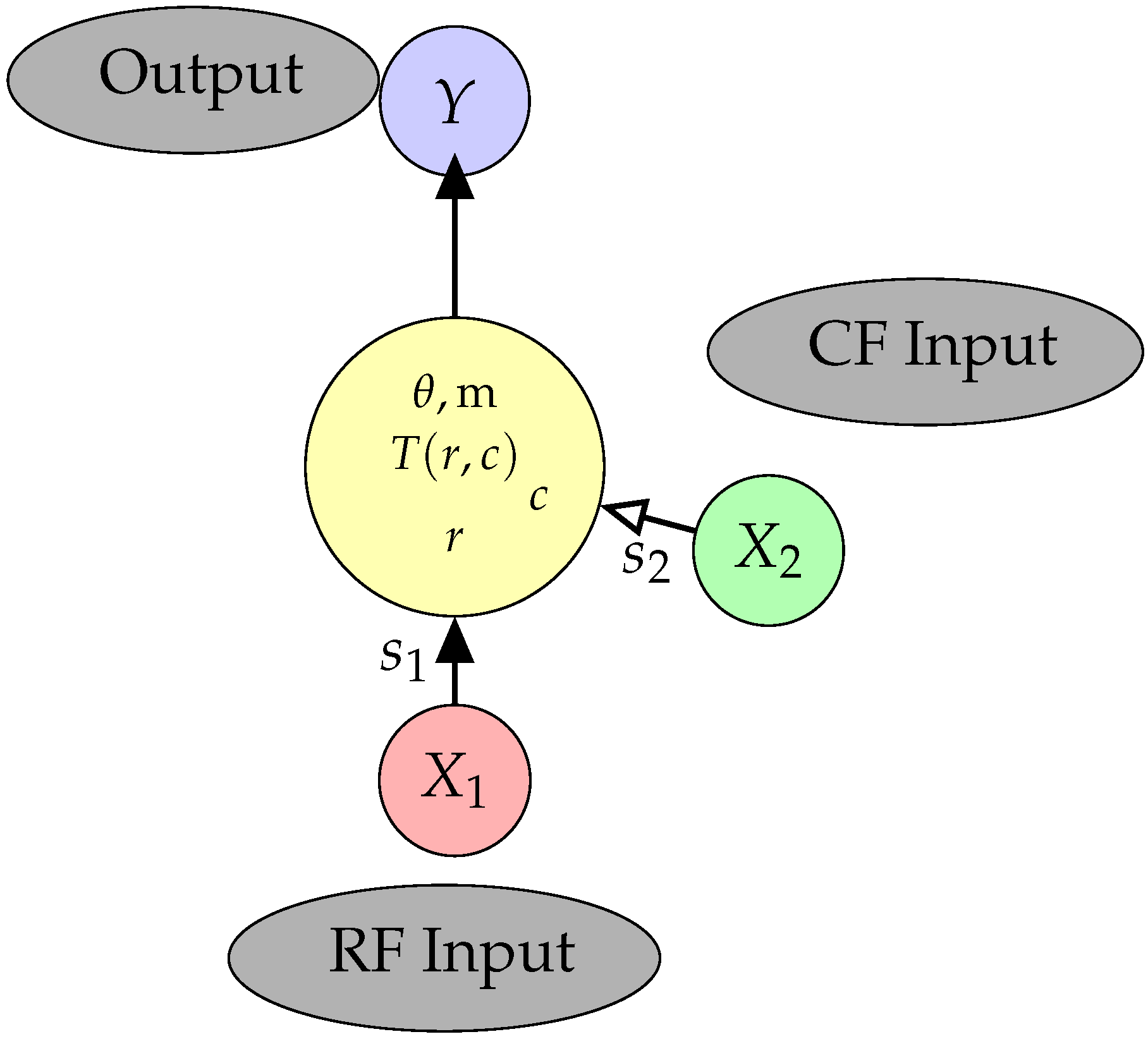
Figure 2.
Classical Shannon measures (in bits), based on additive and modulatory transfer functions, and a correlation between inputs of 0.78.
Figure 2.
Classical Shannon measures (in bits), based on additive and modulatory transfer functions, and a correlation between inputs of 0.78.
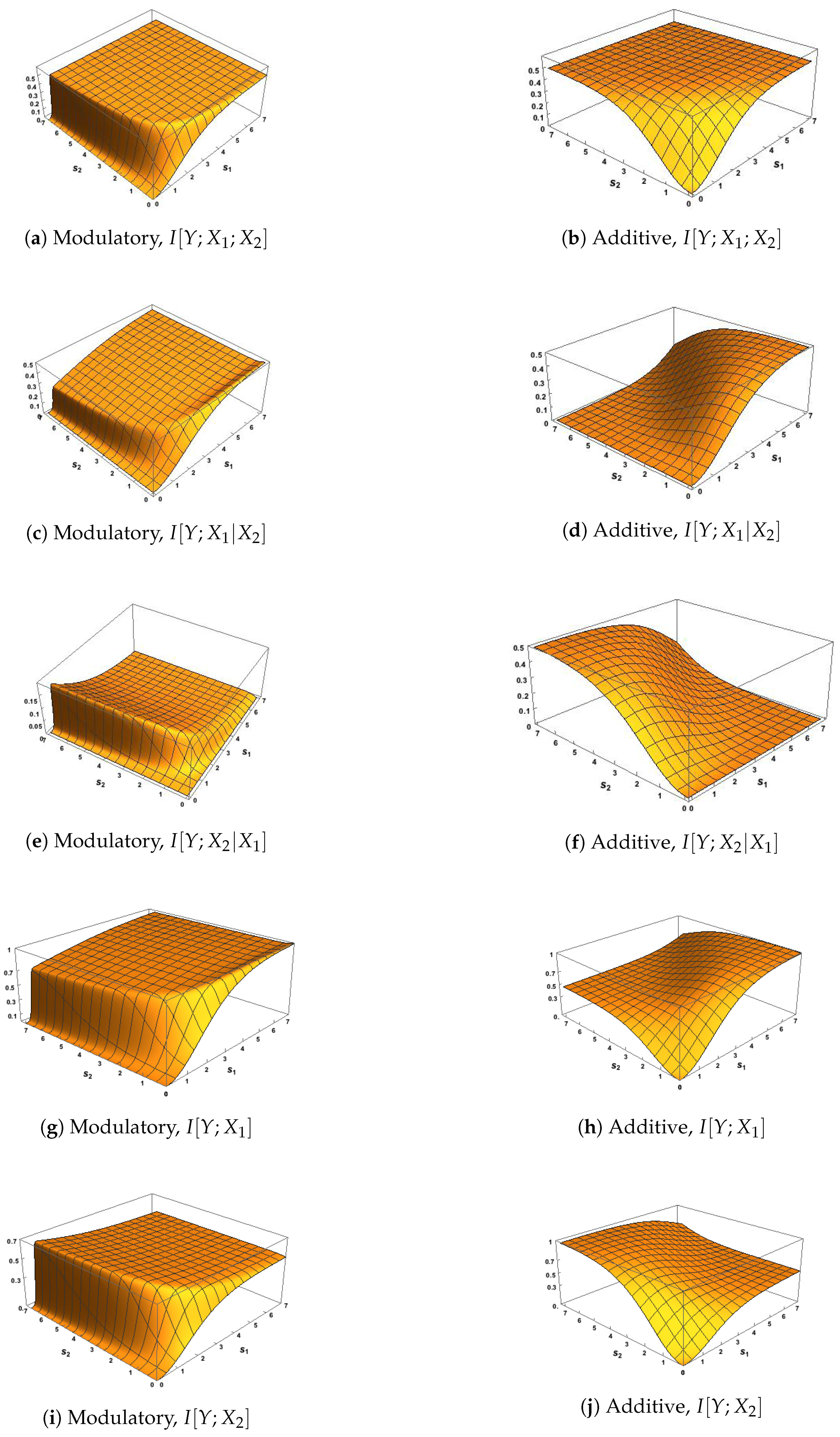
Figure 3.
Classical Shannon measures (in bits), based on additive and modulatory transfer functions, and a zero correlation between inputs.
Figure 3.
Classical Shannon measures (in bits), based on additive and modulatory transfer functions, and a zero correlation between inputs.


Figure 4.
Partial information decomposition (PID) and entropic information decomposition (EID) spectra (in bits), based on additive (A) and modulatory (M) transfer functions for four combinations of signal strengths: 1. (), 2. (), 3. (), 4. (), and two values of the correlation between inputs: 0.78 and zero.

Figure 5.
Ibroja surfaces, based on additive and modulatory transfer functions, and a correlation between inputs of 0.78.
Figure 5.
Ibroja surfaces, based on additive and modulatory transfer functions, and a correlation between inputs of 0.78.

Figure 6.
Ibroja surfaces, based on additive and modulatory transfer functions, and zero correlation between inputs.
Figure 6.
Ibroja surfaces, based on additive and modulatory transfer functions, and zero correlation between inputs.
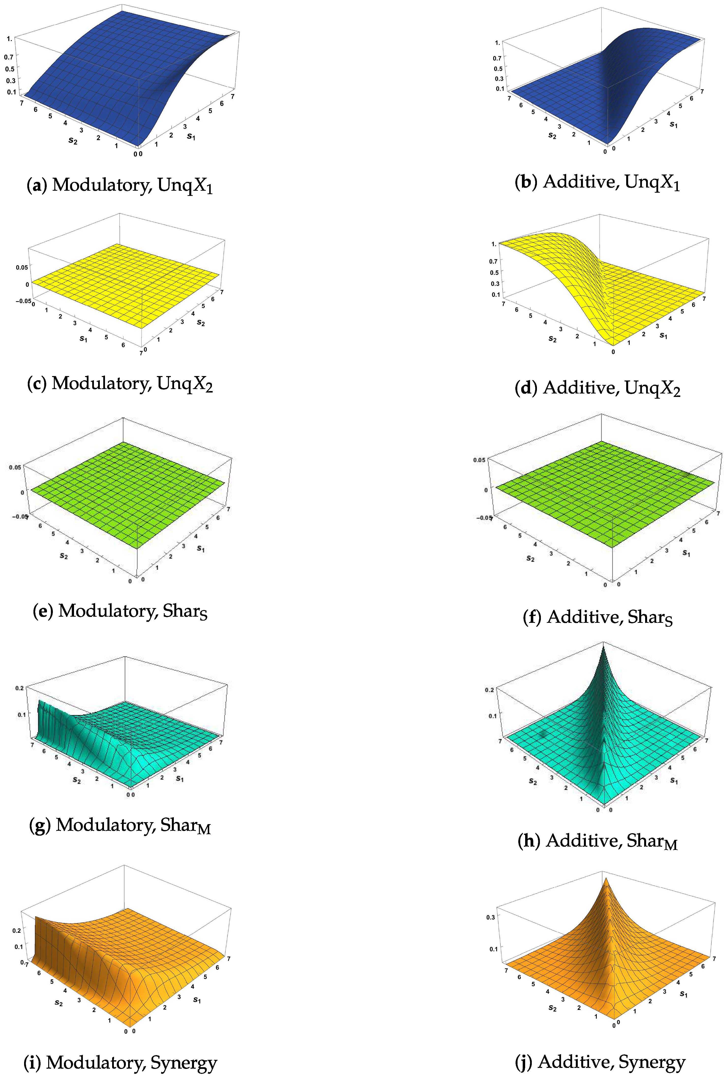
Figure 7.
EID surfaces, based on additive and modulatory transfer functions, and a correlation between inputs of .
Figure 7.
EID surfaces, based on additive and modulatory transfer functions, and a correlation between inputs of .

Figure 8.
EID surfaces, based on additive and modulatory transfer functions, and a zero correlation between inputs.
Figure 8.
EID surfaces, based on additive and modulatory transfer functions, and a zero correlation between inputs.

Figure 9.
Examples of gabor patch stimuli used in the psychophysical experiment. In all conditions, the task was to detect the presence of a centrally presented target gabor.
Figure 9.
Examples of gabor patch stimuli used in the psychophysical experiment. In all conditions, the task was to detect the presence of a centrally presented target gabor.
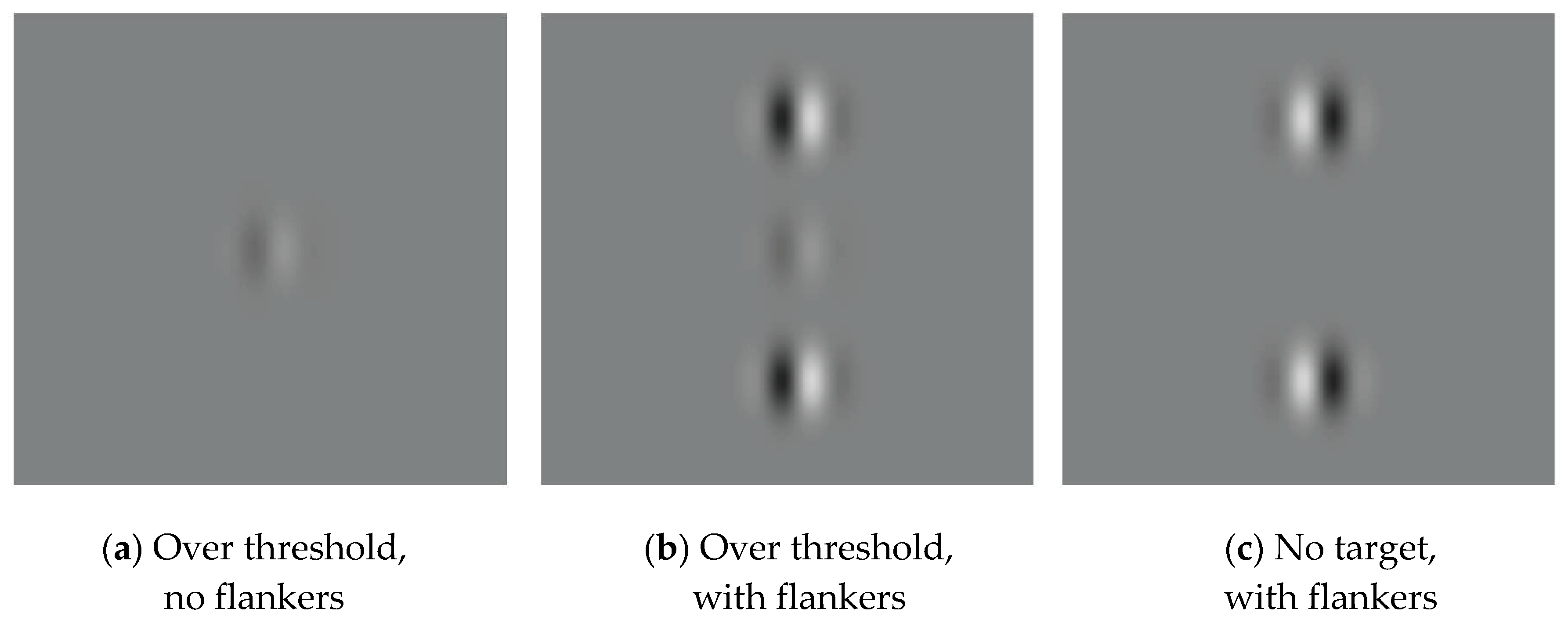
Figure 10.
Partial information decomposition (PID) and EID spectra (in bits) calculated for subject 10 (S10), subject 18 (S18) and the whole group of subjects (G) in the contrast detection experiment calculated at threshold (AT) and over threshold (OT).
Figure 10.
Partial information decomposition (PID) and EID spectra (in bits) calculated for subject 10 (S10), subject 18 (S18) and the whole group of subjects (G) in the contrast detection experiment calculated at threshold (AT) and over threshold (OT).


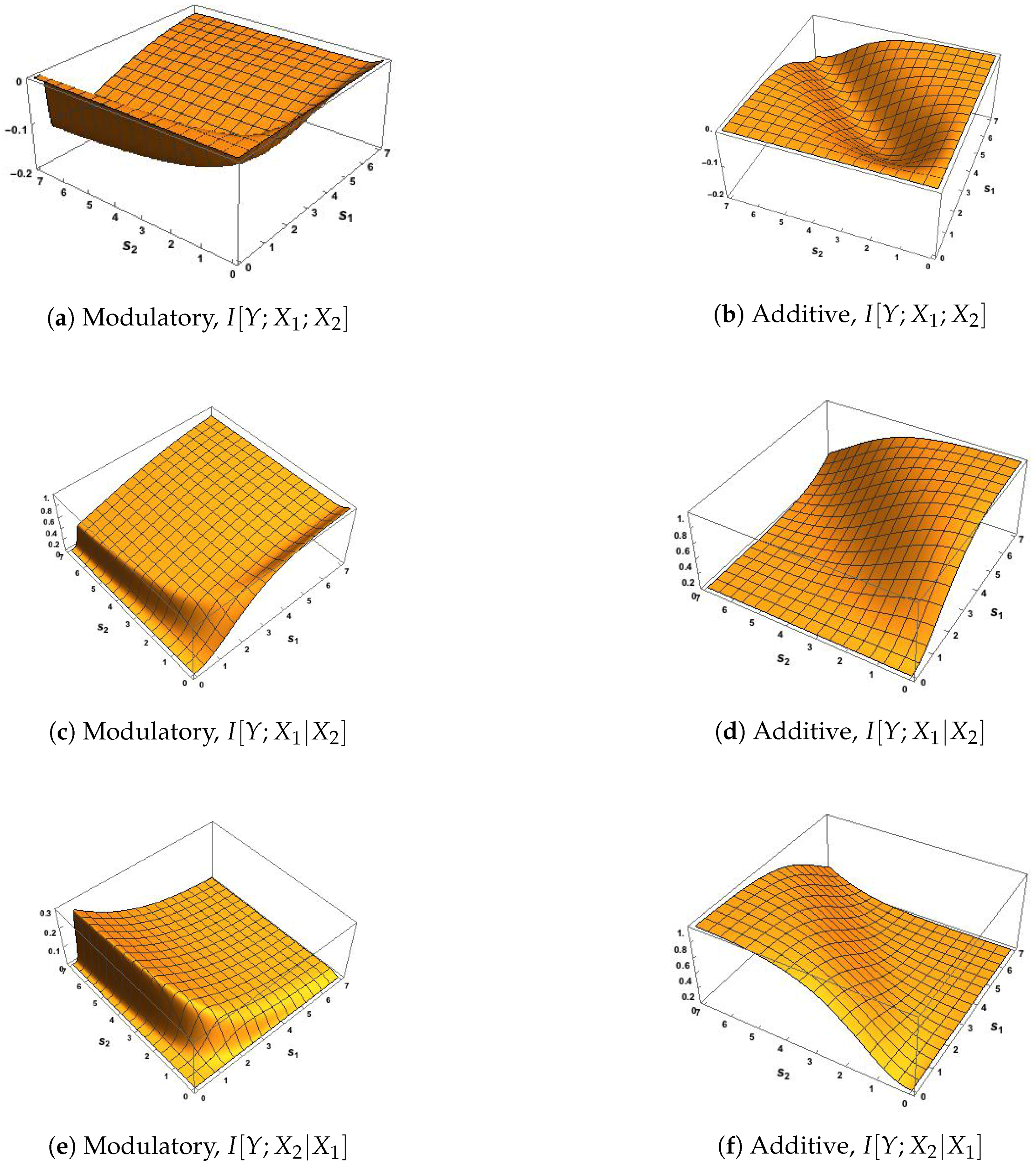
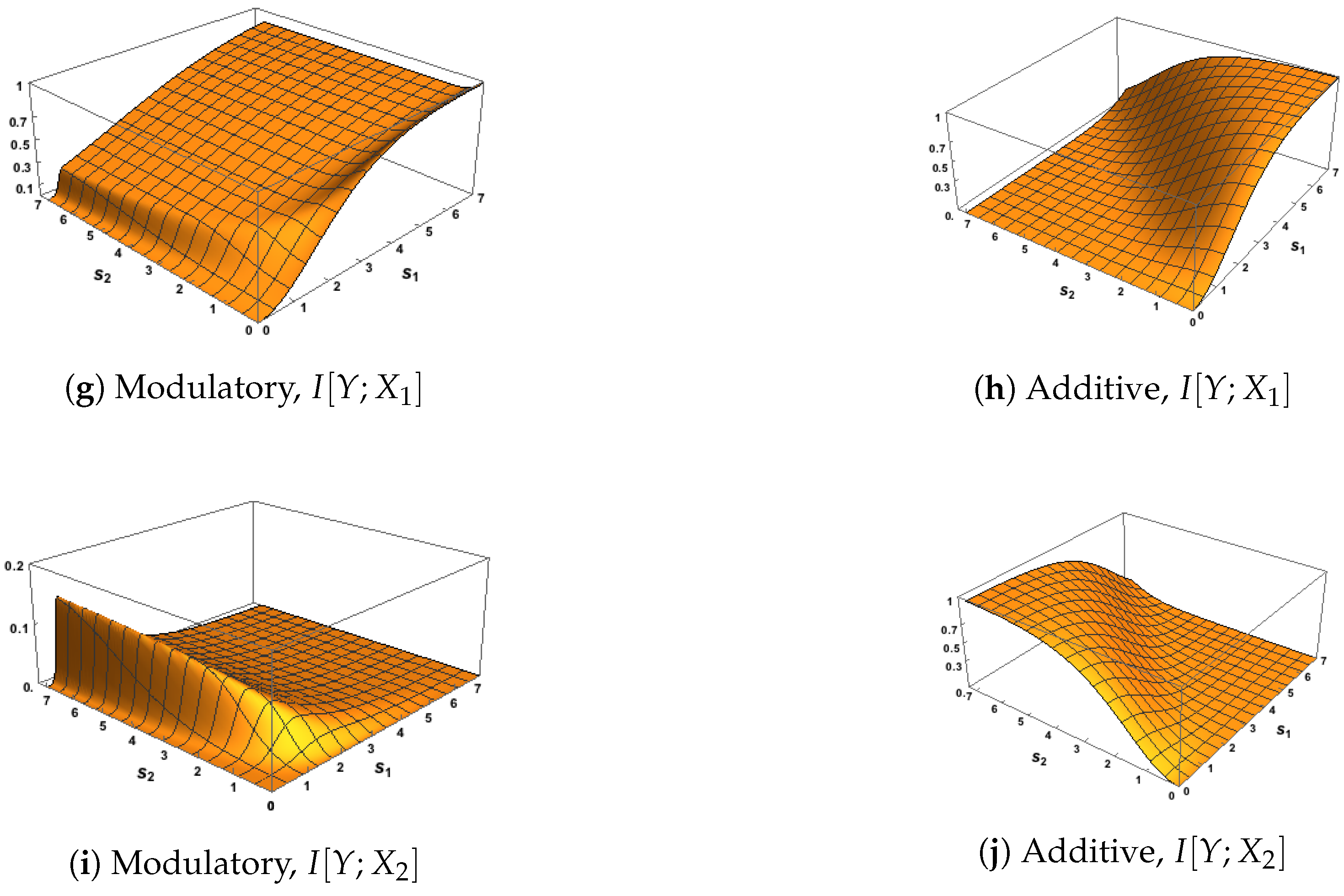
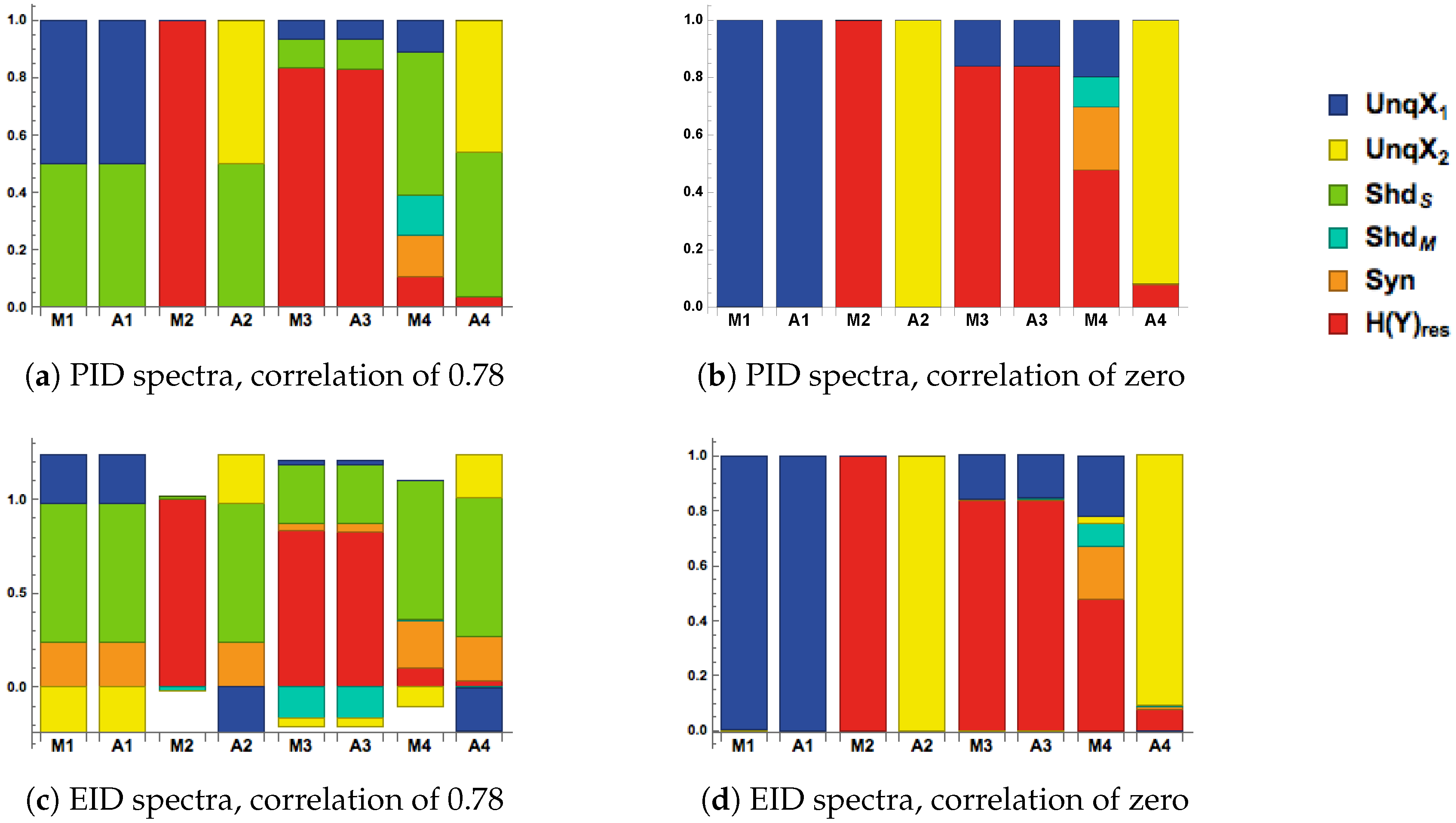
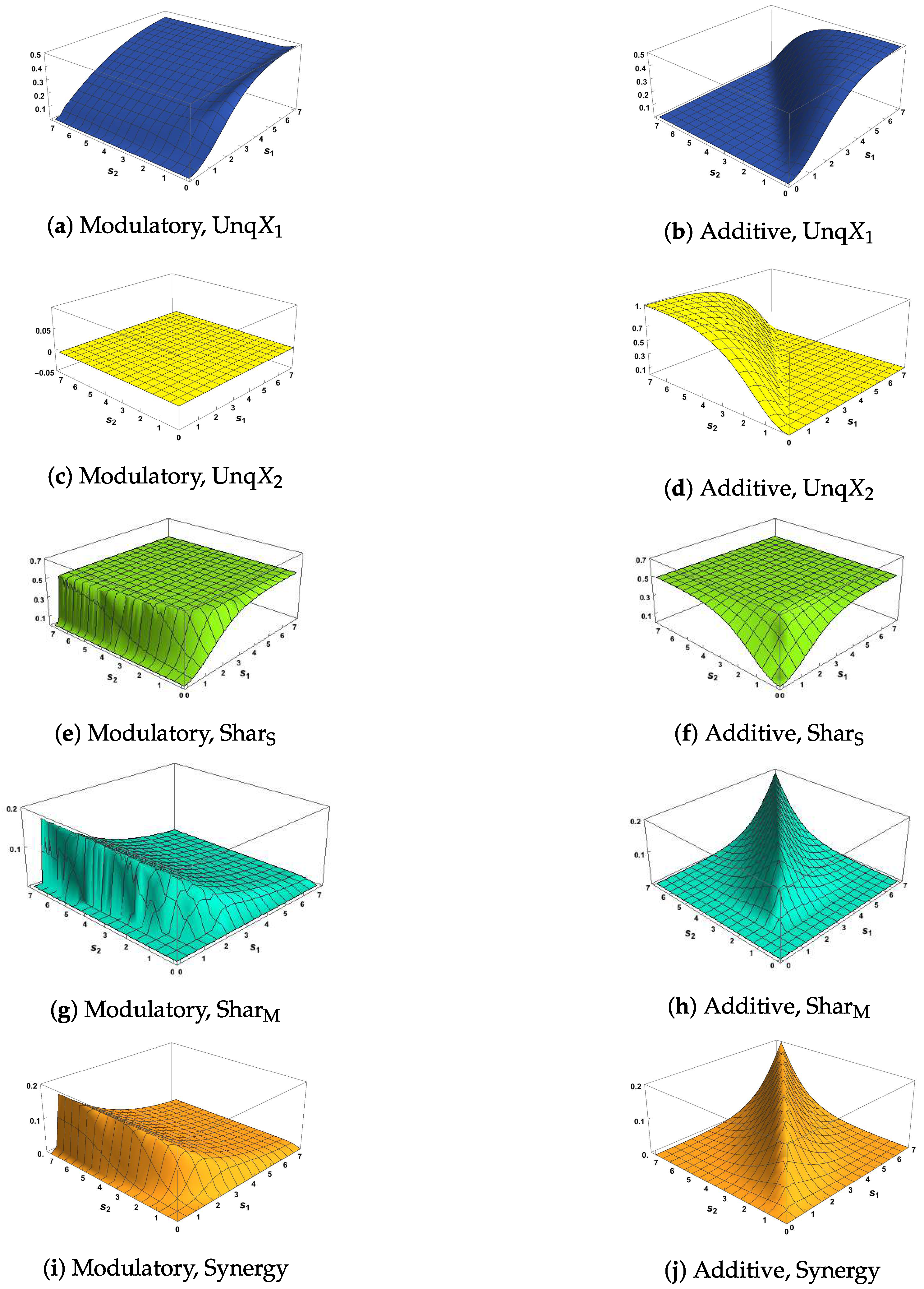
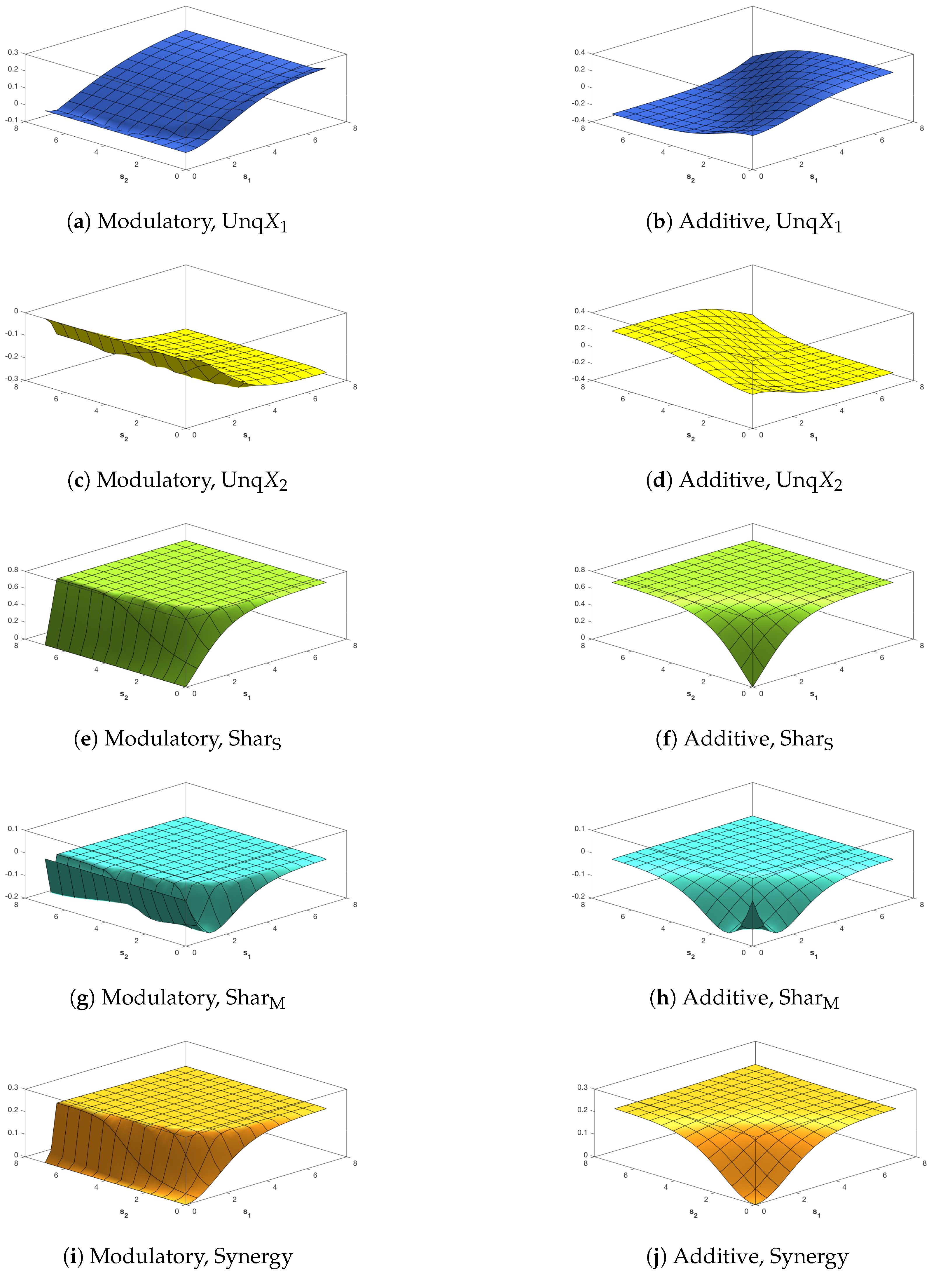
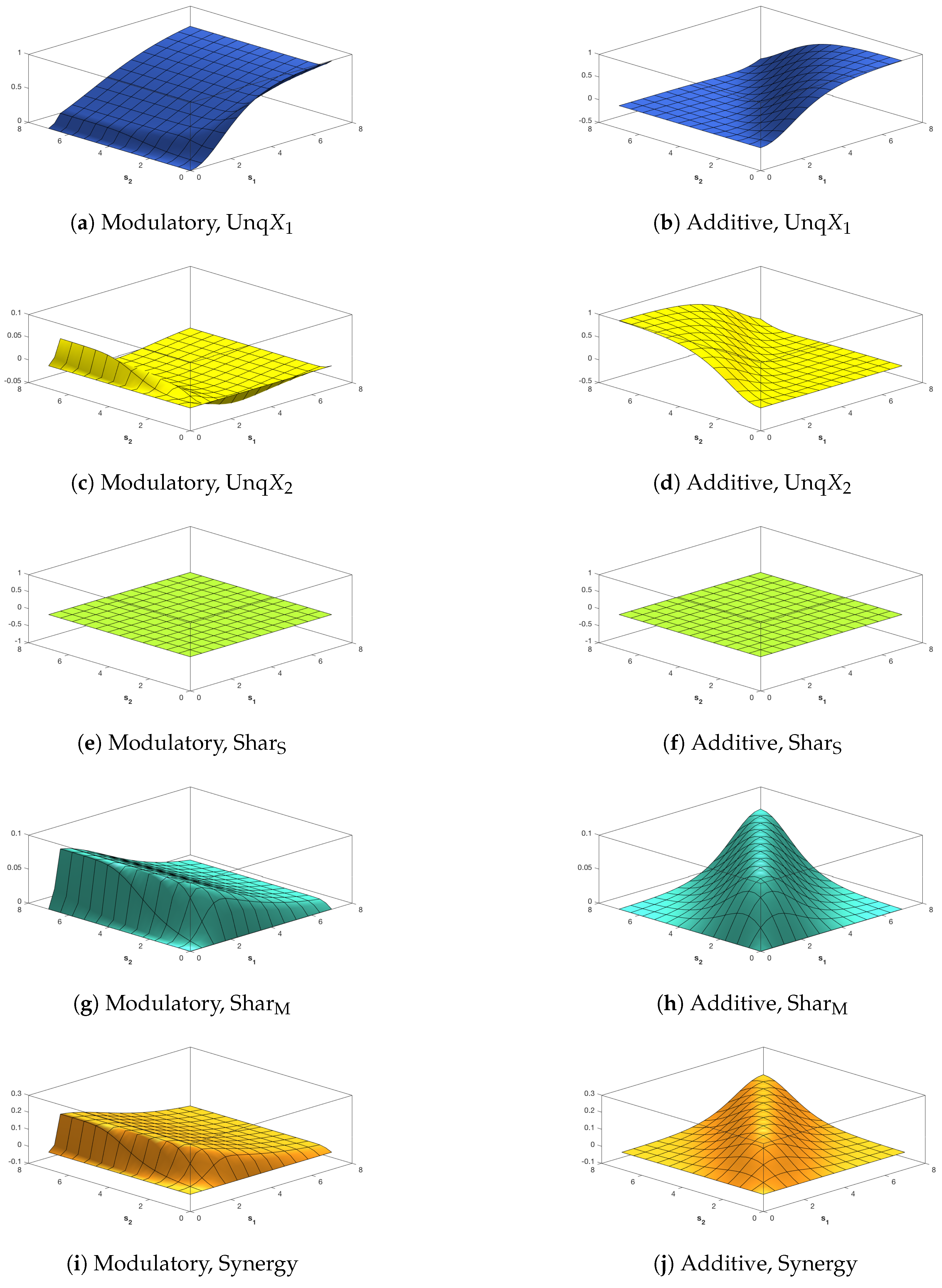
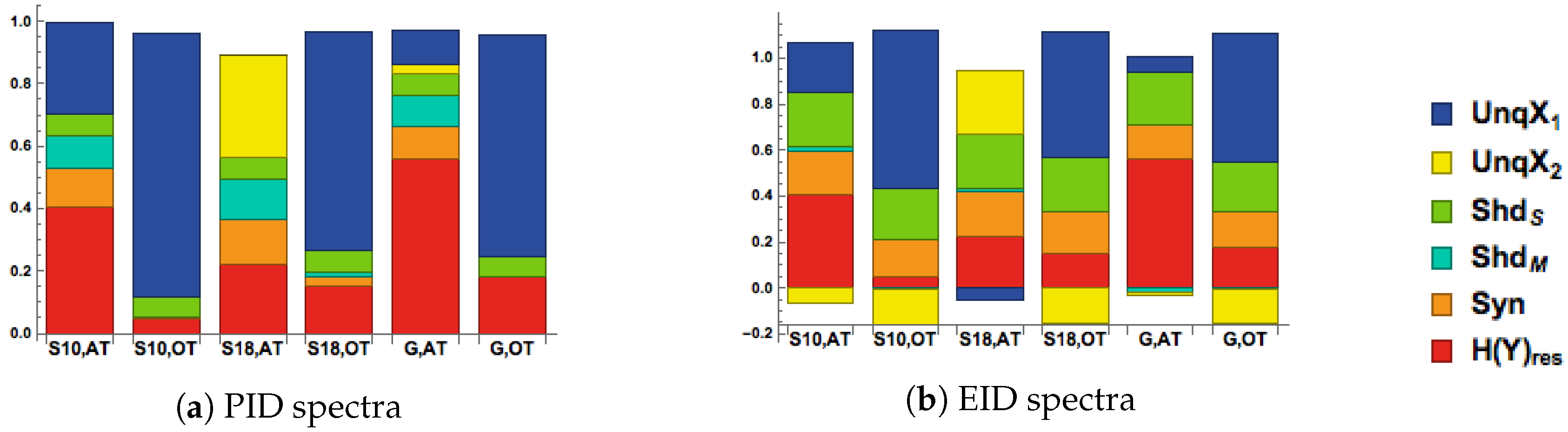
Table 1.
Estimated accuracy, with estimated standard error, for each combination of the three conditions and the absence or presence of flankers.
Table 1.
Estimated accuracy, with estimated standard error, for each combination of the three conditions and the absence or presence of flankers.
| No Target | At Threshold | Over Threshold | |
|---|---|---|---|
| Without Flankers | 0.9096 (0.0273) | 0.8797 (0.0289) | 0.9824 (0.0037) |
| With Flankers | 0.9629 (0.0150) | 0.3766 (0.0532) | 0.9849 (0.0039) |
© 2017 by the authors. Licensee MDPI, Basel, Switzerland. This article is an open access article distributed under the terms and conditions of the Creative Commons Attribution (CC BY) license (http://creativecommons.org/licenses/by/4.0/).
Share and Cite
MDPI and ACS Style
Kay, J.W.; Ince, R.A.A.; Dering, B.; Phillips, W.A. Partial and Entropic Information Decompositions of a Neuronal Modulatory Interaction. Entropy 2017, 19, 560. https://doi.org/10.3390/e19110560
AMA Style
Kay JW, Ince RAA, Dering B, Phillips WA. Partial and Entropic Information Decompositions of a Neuronal Modulatory Interaction. Entropy. 2017; 19(11):560. https://doi.org/10.3390/e19110560
Chicago/Turabian StyleKay, Jim W., Robin A. A. Ince, Benjamin Dering, and William A. Phillips. 2017. "Partial and Entropic Information Decompositions of a Neuronal Modulatory Interaction" Entropy 19, no. 11: 560. https://doi.org/10.3390/e19110560
Note that from the first issue of 2016, this journal uses article numbers instead of page numbers. See further details here.