Complex and Entropy of Fluctuations of Agent-Based Interacting Financial Dynamics with Random Jump


School of Science, Beijing Jiaotong University, Beijing 100044, China
*
Author to whom correspondence should be addressed.
Entropy 2017, 19(10), 512; https://doi.org/10.3390/e19100512
Submission received: 27 July 2017
/
Revised: 8 September 2017
/
Accepted: 21 September 2017
/
Published: 23 September 2017
(This article belongs to the Special Issue Complex Systems, Non-Equilibrium Dynamics and Self-Organisation)
Abstract
:This paper investigates the complex behaviors and entropy properties for a novel random complex interacting stock price dynamics, which is established by the combination of stochastic contact process and compound Poisson process, concerning with stock return fluctuations caused by the spread of investors’ attitudes and random jump fluctuations caused by the macroeconomic environment, respectively. To better understand the fluctuation complex behaviors of the proposed price dynamics, the entropy analyses of random logarithmic price returns and corresponding absolute returns of simulation dataset with different parameter set are preformed, including permutation entropy, fractional permutation entropy, sample entropy and fractional sample entropy. We found that a larger or leads to more complex dynamics, and the absolute return series exhibit lower complex dynamics than the return series. To verify the rationality of the proposed compound price model, the corresponding analyses of actual market datasets are also comparatively preformed. The empirical results verify that the proposed price model can reproduce some important complex dynamics of actual stock markets to some extent.
1. Introduction
The financial market is a complex nonlinear evolving system composed of many interacting agents just as physical systems, and its fluctuation and corresponding absolute returns often represent strong nonlinearity and persistent memory [1,2,3,4,5,6,7,8,9,10,11]. Recently, much effort has gone into the study of reproducing and investigating nonlinear complex dynamics of financial systems for a further understanding the mechanisms of financial markets, and its crucial application in risk management, non-equilibrium derivatives pricing, hedging, forecasting, etc. [2,10,12,13,14,15]. Over the past decade, a considerable volume of agent-based models have been proposed, based on the field of interacting particle systems (or statistical physics systems), to model the main observed stylized facts, such as fat-tailed distribution, volatility clustering, time-dependence, multifractality and complex dynamics [10,16,17,18,19,20,21,22,23,24]. For example, the percolation and oriented percolation are used to construct a financial price model, in which the mutual interaction is imitated by the movement and filtering of fluids through porous materials, and a cluster of percolation is utilized to define the group of investors sharing the same trading attitudes toward the financial markets [17,18]. Stochastic contact process is introduced to construct agent-based financial interacting dynamic system, in which the dissemination of trading attitudes in the financial market is imitated by the epidemic spread process [19]. A novel random financial price dynamics is developed by stochastic exclusion process to study the complex behaviors of financial markets, in which the trading attitude interaction is imitated by the exclusion rules [20]. They are all based on the fact that the financial market is a complex dynamics system comprised of a large number of interacting agents, and these agents interact in complicated ways [6,10], and they try to explain the stylized facts reported in financial time series. Quantifying the complex behaviors of financial signals is one of the most significant topics in understanding financial market dynamics. Entropy, which originates from signal processing, used to quantify the complexity and uncertainty in financial time series and others [25,26,27,28]. Permutation entropy proposed by Bandt and Pompe is a complex measure for arbitrary time series based on analysis of order patterns [29]. Sample entropy, a complex statistics measure of regularity of time series through comparing the number of vector pairs in template vectors of two adjacent integer embedding dimensions, is developed by Richman and Moorman [30]. Fractional sample entropy [31], which is proposed to detect characteristics of fractional order information for complex systems, is utilized to analyze the complex behaviors of datasets in this paper.
Since real stock markets sometimes display violent volatilities and drastic fluctuations, and these jumps have predominant and significant impact on future volatilities, modeling financial market fluctuations with random jumps have become increasingly crucial both for risk management and option pricing [32]. In the present work, the combination of stochastic contact process and compound Poisson process is adopted to construct a novel microscope complex price dynamics, in an attempt to reproduce and characterize the complex dynamics of financial markets. For the proposed compound price model, statistical properties, permutation entropy, fractional permutation entropy, sample entropy, and fractional sample entropy are applied to investigate the fluctuation characters, the fat-tail distribution and complex behaviors of returns and corresponding absolute return time series. Moreover, the comparison results between the actual datasets (Shanghai Stock Exchange (SSE) Composite Index, and Hang Seng Index (HSI)) and the simulation ones confirm that the established nonlinear financial price dynamics can reproduce main complex characteristics of actual market returns.
2. Interacting Price Dynamics with Random Jump
Interacting particle systems have been widely applied to model the financial market dynamics. The behaviors of interacting traders in the financial markets are imitated by particles’ interacting process. These models’ efficiency has been widely testified by a large number of literature. In this section, we construct a novel random complex interacting stock price dynamics by the combination of stochastic contact process and compound Poisson process.
2.1. Stochastic Contact Process
The contact process, one of interacting particle systems [19,33,34], is often thought of as a fundamental model for the spread of some infection. In contact process, infected individuals recover with a constant rate, and healthy individuals become infected with a rate which is proportional to the number of the infected neighbors. Specifically, the stochastic contact model is a continuous time Markov process which belongs to the configuration space . If , the individual at the position x is healthy and will be infected with a rate equal to times the number of the infected neighbors; if , the individual is regarded as infected and becomes healthy at rate 1. For a smooth function f on that depend on finitely many coordinates, the generator of the process is defined as
where if , if , for any . is named the transition rate function and given as
where, denotes Euclidean distance in . Let denotes the state of contact process at time s with the initial infected set . Further, let be the state of at time s with the initial single point infected set . One of the most important features of the contact process is that survival and extinction can be both occur, and which one occurs depends on the value of rate . There is a critical value, which is defined as
where denotes the cardinality of a finite set A. If , the contact process is said to die out, namely, ; otherwise, for , it is said to survive. More generally, we consider the initial probability distribution of infected individuals as , the product measure with probability () at the initial moment, namely, each individual is independently infected with probability , and denoted as for simplicity.
2.2. Modeling Financial Price Model
In this section, we develop a novel agent-based price dynamics by the combination of contact process and compound Poisson process with normally distributed jumps, which represent the fluctuations caused by the spread of the investors’ trading attitudes and the random jump fluctuations caused by the macroeconomic environment, respectively. Firstly, we assume that the stock price fluctuations partly result from the investors trading attitudes toward the stock market, and suppose that the trading attitude is represented by the viruses of the contact model, which accordingly classify the market investors with buying attitude, selling attitude and neutral attitude, respectively. Considering a model of auctions in a security market, assume that each investor can trade the stock several times each day , but at most one unit of security each time. Let l be the length of trading time in each trading day, we denote the security price at time s in the t-th trading day by where . Suppose that the security market consists of (M is large enough) investors, who are located in lattice (similarly for d-dimensional lattice ). At the beginning of every trading day, suppose that the investors at the infected sites have same trading attitudes. Then, we define a random variable for these investors, suppose these investors take buying attitude (), selling attitude () or neutral attitude () with probability , or , respectively. Then, these investors send bullish, bearish or neutral attitudes to their nearest neighbors according to the one-dimension contact dynamic mechanisms. Infected investors can affect their neighbors, or the trading attitudes can be spread, which is assumed as one of the main factors for price fluctuations. For a fixed , we define
where is the cardinal number of investors who take buying position or selling position at time s with initial distribution , represents trading attitudes in t-th trading day, and, hence, represents the aggregate demand in t-th trading day. From the above definitions and References [10,19,21], the stock price evolution at t-th trading day is given as
where the coefficient is named depth parameter of the security market in this work, which measures sensitivity of price fluctuation in response to the aggregate demand. Thus, we have
where is the initial stock price at time .
Then, we pay attention to the random jump fluctuations. Suppose is a Poisson process with intensity , is an independent identical distributed (i.i.d.) sequence with normally distributed jumps, and and are independent. The stock return jump amplitude at k-th Poisson point is . Here, is defined as the k-th sample value of a standard normal distribution. The compound Poisson jump of the price is given by
where the coefficient measures sensitivity of price fluctuation in response to macroeconomic environment.
We assume that the fluctuations of a security price is determined mainly by two parts, and . We define the stock price on , which describes the behavior of all markets investors. More specifically, the stock price at t-th trading day, for a fixed , is defined as
where is initial stock price at time 0, and parameters . Now, we discuss the price process with the continuous time, which are defined from Equation (9). The normalized process is defined by
where denotes the integral part of a real number , and is a random variable which denotes the area under the . From References [10,19], the formula of stock logarithmic return is defined as
3. Probability Distributions of the Price Model
Considering stock returns in an interval time are autocorrelated [4,10], for the interacting part of the model, the “area” may represent the situation on this stock during the time from 0 to n, including the investors’ prediction, company prospect and benefit, trends, political event, economic policy, etc. If “area” is positive, there may have a positive influence on some market participants so that they are likely to take buying positions. In this paper, we only consider the case that the “area” is positive when n is large enough, similarly for the opposite case. In the following, with the condition , the limiting probability distribution of random process is given. When is large enough and , the finite dimensional distribution of normalized conditional return process
converges to the corresponding distribution
where is a standard Brownian motion, is the degree of fluctuation of the stock price, and is the local tendency of the stock price process. The proof is based on Section 4 of [35], whose strategy of proof is from the theory in [36,37,38]. For the jump part of the model, since is a compound Poisson process, then is a Lévy process [39,40,41]. For real-valued Lévy processes, the characteristic function of its increments follows the Lévy–Khinchine formula
where , , m and are continuous functions of t. From the combination of above two parts, and by Equations (12) and (13), we can deduce that the distribution of the proposed model given in Equation (9) has the Lévy type distribution.
4. Empirical Research for Financial Price Dynamics
In this section, we investigate the nonlinear complex behaviors of the proposed compound financial price dynamics. To obtain a robust result, actual market datasets (Shanghai Stock Exchange (SSE) composite index and Hang Seng Index (HSI)) are comparatively considered with the simulation ones, the selected daily closing prices for the period from 28 June 1995 to 31 May 2017 with 5320 data points (some slight differences exist for different non-trading days between the two markets, and some one-day missing values are supplemented by linear interpolation). The time series are available on the Yahoo Finance website (https://finance.yahoo.com). For simplicity, the corresponding empirical experiment is performed by computer simulation for different infection rates in contact process, and different intensity in compound Poisson process. In the following, we set the time length of analysis to 5320 and initial probability to (namely, each individual is independently infected with probability ) in contact process to gain simulation datasets.
4.1. Basic Statistical Properties of Returns
The statistical analysis of the financial returns and the corresponding absolute return series has attracted the interest of many researchers for their wide application in asset allocation, asset pricing, risk management, stock return volatility forecasting, etc. [2,10,12,13,14,15]. Recent empirical works have reported that the empirical probability distributions of financial returns are believed to deviate from a Gaussian distribution, and they usually exhibit more leptokurtic and fatter tails than the Gaussian case, which is usually called “fat-tail” distribution, and may be explained as the result of the herd effect of investors in the security markets or illiquidity. A highly leptokurtic distribution is characterized by a narrower and larger maximum, and by fatter tails than a Gaussian one [10]. The kurtosis, which is one of the most important statistics to describe leptokurtic, is exhibited in Table 1. When the kurtosis of a series is larger than 3, which is the kurtosis of a Gaussian distribution, there exist fat tails in the probability distribution. Moreover, the descriptive statistics, the Kolmogorov-Smirnov (K-S) test and Anderson-Darling (A-D) test of normalized returns of the actual marketdatasets and the simulation ones are also exhibited in Table 1 [42]. In the K-S test of the corresponding normalized returns, the signification level is 5%, and the lengths of returns are 5320, the critical values are the same at . The K-S test returns the logical value if it rejects the null hypothesis that the distribution of normalized returns follows the standard normal distribution at the given significance level, while if it cannot. In the A-D test of the returns, the hypothesized distribution is normal distribution in this paper, the signification level is also 5%, and the corresponding critical values are . The A-D test returns the logical value if it rejects the null hypothesis that the distribution of returns follows a given probability distribution (here, normal distribution) at the given significance level, while if it cannot [42].
According to the empirical results in Table 1, we can find that the tail distributions of the simulative datasets and the actual ones are deviating from the Gaussian case, the kurtosis are larger than 3. Moreover, in K-S test and A-D test, all the logical values are 1, and all the stats are larger than the corresponding critical value, so the null hypothesis that the distribution of the simulative datasets and the actual ones follow the normal distribution can be rejected at the significance level 5%. It is obvious that the actual datasets and the simulation ones display similar fat-tail and leptokurtic attributes. We also find that the kurtosis isincreasing steadily from to with increasing from to and fixed , which imply that the fat-tail behavior is more significantly as increases. The reason of this increasing is that the rate represents the rate of attitude spread in the price dynamics, and the increasing of implies the interaction among the investors becomes more and more active, which is supposed to bring the herd behavior of the security market, and usually results in the fat-tail distribution for the returns. There are similar patterns for and , but larger kurtosis than the case of , which may be explained that represents the rate of Poisson jumps; that is, a larger shows more large fluctuations and directly leads to fat-tail phenomenon of the returns.
Moreover, the empirical probability density distributions of the simulation datasets with are presented in Figure 1 with comparison to a Gaussian distribution. The patterns of these curves also show that the actual datasets and the simulated ones deviate from the Gaussian. It is transparent that the simulation datasets exhibit the similar fat-tail and peak distributions to the actual ones.
4.2. Fractional Permutation Entropy
Permutation entropy, proposed by Bandt and Pompe, is a complex measure for arbitrary time series based on analysis of order patterns [29]. Consider a time series , comparing n-dimension vector , suppose it has permutation , and all n! permutations of order n which are considered as possible order types of n different numbers. For each permutation , the relative frequency is determined as
where n and denote the embedding dimension and the time delay, respectively. The permutation entropy of order is defined as
where the sum runs over all permutations of order n. The permutation entropy is between 0 and for , when all the permutations have same frequency, reaches its maximum.
Permutation entropy of returns and absolute returns for of simulation datasets and actual datasets with are exhibited in Table 2. We can find that all the permutation entropy values are close, the permutation entropy of returns is slightly increasing from to with increasing from to and fixed and , which means that the behavior of returns is more complex as increases. The reason for this increase is that the rate represents the rate of attitude spread, and the increasing of implies that the interaction among the investors becomes more frequent, which is supposed to bring more random order patterns and temporal information, and hence lead to more complex dynamics. There are similar patterns for and , but with larger permutation entropy than the case of . This may be explained as a larger shows more frequent violent fluctuation to the stock price. Additionally, the permutation entropy values of absolute returns are slightly smaller than those of returns , which represents that the absolute return series exhibit less order permutation patterns, larger correlation, and hence are easier to predict than the return series.
A generalized expression of permutation entropy is brought with approaches in fractional calculus by References [43,44]. Fractional permutation entropy (FPE), a modified permutation entropy, is proposed to detect fractional order characteristics for complex system.
Figure 2 depicts FPE curves versus from to with step size of for the actual market datasets and the simulation ones with and ((a) for and (b) for ). We can find that all curves evolve along similar shape. In Figure 2, the FPE values track with larger lie above the ones with smaller . It indicates that, when increases, the FPE increases, which means that the dynamics of system become more complex as increases. Because the rate relates to the speed of investors react to the security market, as increases, the market will become more swarming and the investors are more likely to group together which lead to large fluctuations as a result.
4.3. Fractional Sample Entropy
Sample entropy proposed by Richman and Moorman [30], which is independent of data length and exhibits relative consistency, is a complex statistics method of time series through comparing of vector pairs in template vectors of two adjacent embedding dimension. Considering a time series , the state vector is defined as (), where , represents the time delay (set in the following for simplicity) and m represents the embedding dimension, respectively. The underlying dynamics of time series are fully embedded in the m-dimensional phase space . The embedding theorem [45] guarantees a full knowledge of a system contained in the time series of any one measurement and a proxy for the full multivariate phase space that can be constructed from the time series. Two vectors, and , are considered as close if their distance is smaller than a given tolerance level . Let represents the number of vectors (where to exclude self-matches) that are close to the vector . Then, the probability that any vector is close to the vector within a tolerance level is defined as
The average of the is given as
which represents the frequency that any two vectors are within of each other. Then, the sample entropy of time series is given as
Although m and are vital in calculating the sample entropy, no guidelines exist for optimizing their values. The rule accepted widely is that and values of m of 1 or 2. We calculate the fractional sample entropy for all datasets with parameters and , represents the standard deviation of the considered time series, which is the usually chosen parameters combination [31].
Sample entropies of returns and absolute returns of simulation datasets and actual datasets with are exhibited in Table 4. For every fixed parameter set, as value increases, the sample entropy increases, which means that the sample entropy values for larger are larger than those for smaller , which shows that a larger leads to larger fluctuation, larger difference in number of vector pairs in template vectors of two adjacent embedding dimension, less self-similarity in data series, hence leads to more complex dynamics. We also find that sample entropies for and are slightly less than those for , which means that higher frequency of jumps leads to more diversified template vectors. Meanwhile, the sample entropies of absolute returns are slightly smaller than those of returns , which displays that the absolute return series exhibit more self-similarity, lower complex dynamics than the return series.
The fractional sample entropy, a modified sample entropy approximation based on the methods in References [30,43], is developed to detect characteristics of fractional order information for complex dynamics [31]. The fractional sample entropy (FSE) of time series is then defined as Reference [31]
The FSE method is applied to study the complex behaviors of the actual datasets, the simulation ones, the empirical results with Gaussian are exhibited in Table 5 and Table 6 and Figure 2. Table 5 displays the FSE of returns with fractional exponent form to with step size of for different values of and . For every fixed parameter set, as value increases, the FSE firstly increases and then decreases. All the FSE values of simulation datasets and actual ones are less than the corresponding FSE values of Gaussian, which displays that they are deviating from the Gaussian series. Meanwhile, for every fixed parameter set, as value increases, the FSE increases, which means that the FSE for larger are larger than those for smaller , which shows that a larger leads to more complex dynamics. We also find that the FSE for and are slightly less than those for , which means that higher frequency of jumps leads to more complex behaviors. Additionally, comparing Table 6 with Table 5, we find that the FSE values of absolute returns are observably less than the corresponding FSE values of returns (except for Gaussian), which means that the absolute return series exhibit lower complexity than the return series.
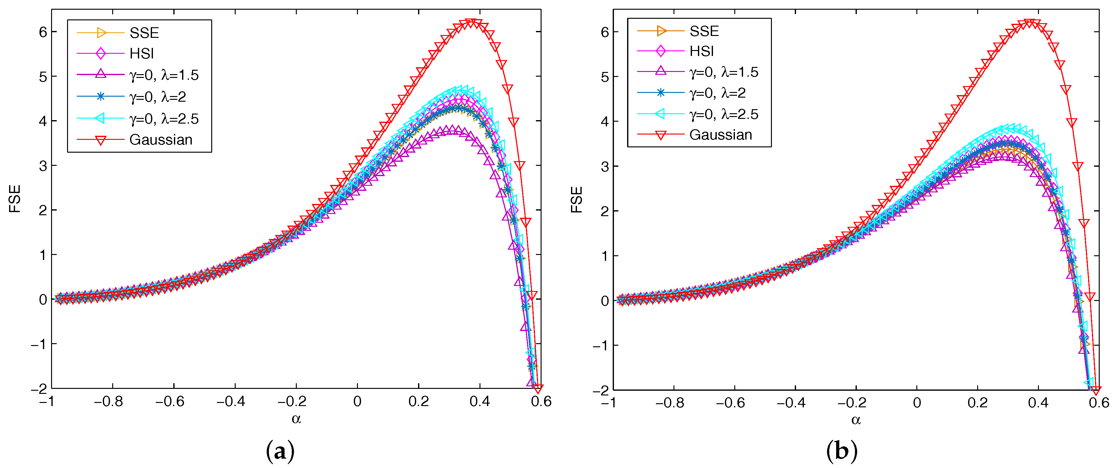
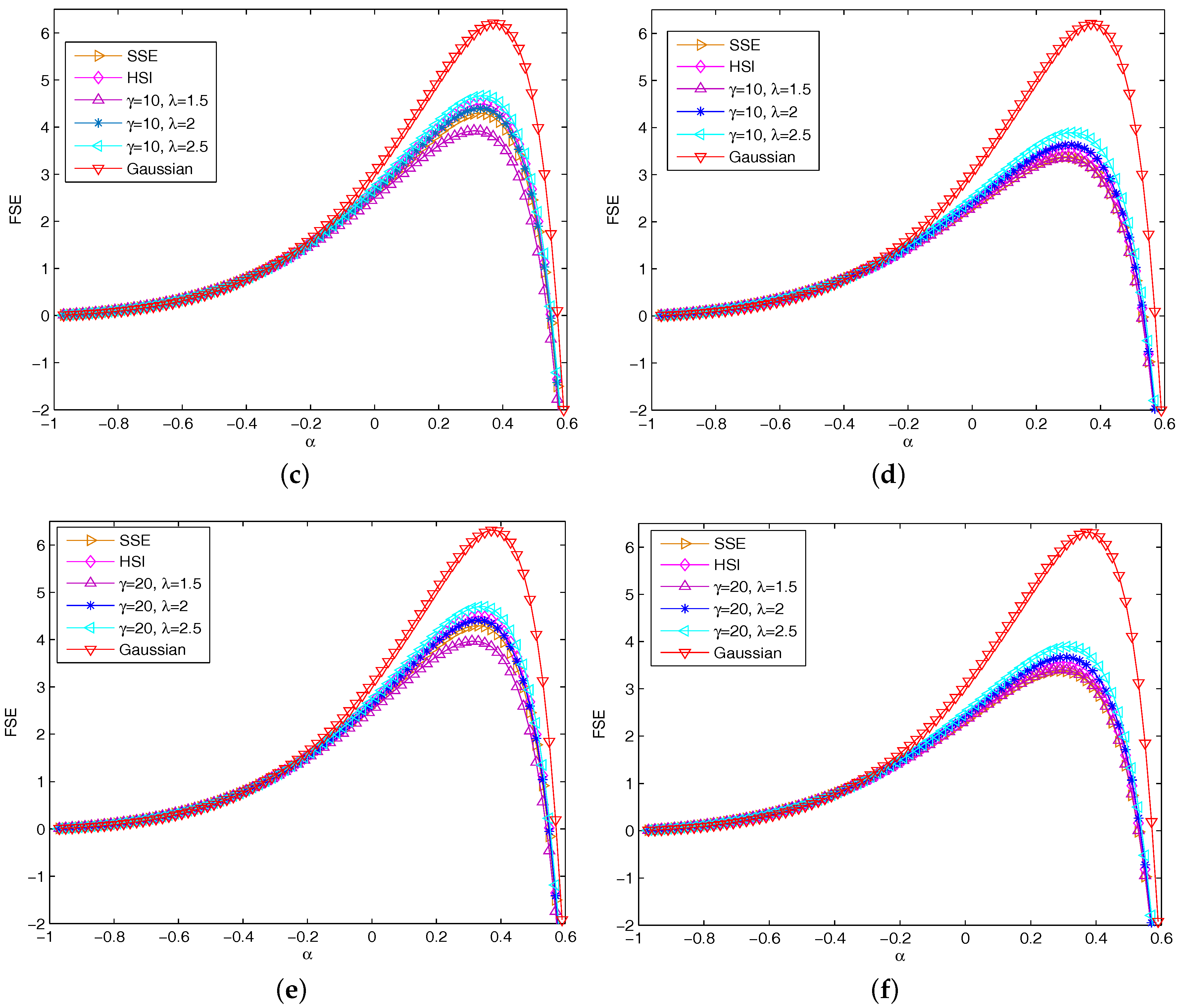
Figure 3 depicts FSE curves versus for the actual market datasets and the simulation ones, ranges from to with step size of . Figure 3a depicts the FSE curves of returns of the SSE, the HSI, and the financial price model for , and with fixed . All curves evolve along similar shape, as value increases, the FSE firstly increases and then decreases. The FSE values of Gaussian lies above others, and, as can be seen, all datasets are deviating from the Gaussian. In Figure 3a, the FSE track with larger lies above the ones with smaller . It indicates that, when increases, the FSE increases, which means that the dynamics of system become more complex as increases. Because the rate relates to the speed of investors react to the security market, as increases, the market will become more swarming and the investors are more likely to group together which lead to large fluctuations as a result. Figure 3b depicts the FSE curves of absolute returns of the actual datasets and simulation ones. Being compared with Figure 3a,b has similar dynamics behaviors. Figure 3b illustrates that except for Gaussian series, the FSE of absolute return series of actual datasets and simulation ones significantly decrease, which means that absolute return series exhibit lower complexity than return series. Figure 3c,d and Figure 3e,f depict the FSE curves of returns and absolute return series with and , and have similar patterns with Figure 3a,b.
5. Conclusions
In the present paper, a novel agent-based complex price dynamics is introduced by the combination of contact process and compound Poisson process with normally distributed jumps, which concern with the fluctuations caused by the spread of the investors’ attitudes and random jump fluctuations caused by macroeconomic environment, respectively. Then, we investigate and analyze the statistical behaviors of returns of the proposed model by descriptive statistics, K-S test and A-D test. The results show that the proposed price dynamics displays some stylized facts reported in financial time series. Further, to better understand complex dynamics of the proposed model, entropy analyses including permutation entropy, fractional permutation entropy, sample entropy and fractional sample entropy are preformed. The empirical results show that absolute return series exhibit less complex dynamics than fluctuation ones. A large is more likely to lead to complex dynamics, since the rate relates to the speed of attitude interaction in the security market, as increases, the market will become more swarming which lead to large fluctuations as a result. Furthermore, larger almost have larger entropy, since represents the rate of Poisson jumps, a large is more liable to trigger large fluctuation and directly lead to fat-tail and complex dynamics. Moreover, we choose the daily returns of SSE and HSI as the actual market datasets. Through the comparisons of the above analyses for the actual datasets and the simulation ones, the simulation datasets derived from the nonlinear stochastic interacting price model have similar statistical and complex dynamics with the actual markets, which indicates that the present financial price dynamics model could grasp some natural features of actual markets to some extent.
Acknowledgments
The authors were supported by National Natural Science Foundation of China Grant No. 11371050 and 71271026.
Author Contributions
YiduanWang and Wei Zhang collected the data, designed and performed the numerical analyses, wrote the main text, and generated the figures. YiduanWang, Wei Zhang, Jun Wang and Shenzhou Zheng reviewed the economic background and put the work into context. Jun Wang and Shenzhou Zheng reviewed the graph-theoretic background. Jun Wang and Shenzhou Zheng supervised the project. All authors have read and approved the manuscript.
Conflicts of Interest
The authors declare no conflict of interest.
Abbreviations
The following abbreviations are used in this manuscript:
| SSE | Shanghai Stock Exchange |
| HSI | Hang Seng Index |
| FPE | fractional permutation entropy |
| PSE | fractional sample entropy |
References
- Black, F.; Scholes, M. The pricing of options and corporate liabilities. J. Polit. Econ. 1973, 81, 637–654. [Google Scholar] [CrossRef]
- Calvet, L.; Fisher, A. Multifractal Volatility: Theory, Forecasting, and Pricing; Academic Press: New York, NY, USA, 2008. [Google Scholar]
- Gabaix, X.; Gopikrishnan, P.; Plerou, V.; Stanley, H.E. A theory of power-law distributions in financial market fluctuations. Nature 2003, 423, 267–270. [Google Scholar] [CrossRef] [PubMed]
- Preis, T.; Kenett, D.Y.; Stanley, H.E.; Helbing, D.; Ben-Jacob, E. Quantifying the Behavior of Stock Correlations under Market Stress. Sci. Rep. 2012, 2, 752. [Google Scholar] [CrossRef] [PubMed]
- Trivellato, B. Deformed Exponentials and Applications to Finance. Entropy 2013, 15, 3471–3489. [Google Scholar] [CrossRef]
- Lux, T. Financial Power Laws: Empirical Evidence, Models and Mechanisms; Cambridge University Press: Cambridge, UK, 2008. [Google Scholar]
- Niu, H.; Wang, J. Volatility clustering and long memory of financial time series and financial price model. Digit. Signal Process. 2013, 23, 489–498. [Google Scholar] [CrossRef]
- Münnix, M.C.; Shimada, T.; Schäfer, R.; Leyvraz, F.; Seligman, T.H.; Guhr, T.; Stanley, H.E. Identifying States of a Financial Market. Sci. Rep. 2012, 2, 6449. [Google Scholar] [CrossRef] [PubMed]
- Shang, Y. An agent based model for opinion dynamics with random confidence threshold. Commun. Nonlinear Sci. Numer. Simul. 2014, 19, 3766–3777. [Google Scholar] [CrossRef]
- Mantegna, R.N.; Stanley, H.E. An Introduction to Econophysics: Correlations and Complexity in Finance; Cambridge University Press: Cambridge, UK, 1999. [Google Scholar]
- Mandelbrot, B.B. Fractals and Scaling in Finance; Springer: New York, NY, USA, 1997. [Google Scholar]
- Gaylord, R.; Wellin, P. Computer Simulations with Mathematica: Explorations in the Physical, Biological and Social Science; Springer: New York, NY, USA, 1995. [Google Scholar]
- Ilinski, K. Physics of Finance, Gauge Modeling in Nonequilibrium Pricing; Wiley: New York, NY, USA, 2001. [Google Scholar]
- Lux, T.; Marchesi, M. Scaling and criticality in a stochastic multi-agent model of a financial market. Nature 1999, 397, 498–500. [Google Scholar] [CrossRef]
- Mills, T.C. The Econometric Modeling of Financial Time Series, 2nd ed.; Cambridge University Press: Cambridge, UK, 1999. [Google Scholar]
- Ross, S.M. An Introduction to Mathematical Finance; Cambridge University Press: Cambridge, UK, 1999. [Google Scholar]
- Yu, Y.; Wang, J. Lattice-oriented percolation system applied to volatility behavior of stock market. J. Appl. Stat. 2012, 39, 785–797. [Google Scholar] [CrossRef]
- Stauffer, D.; Penna, T.J.P. Crossover in the Cont-Bouchaud percolation model for market fluctuation. Physica A 1998, 256, 284–290. [Google Scholar] [CrossRef]
- Yang, G.; Wang, J.; Deng, W. Nonlinear analysis of volatility duration financial series model by stochastic interacting dynamic system. Nonlinear Dyn. 2015, 80, 701–713. [Google Scholar] [CrossRef]
- Zhang, W.; Wang, J. Nonlinear stochastic exclusion financial dynamics modeling and complexity behaviors. Nonlinear Dyn. 2017, 88, 921–935. [Google Scholar] [CrossRef]
- Zhang, W.; Wang, J. Nonlinear stochastic exclusion financial dynamics modeling and time-dependent intrinsic detrended cross-correlation. Physica A 2017, 482, 29–41. [Google Scholar] [CrossRef]
- Niu, H.L.; Wang, J. Entropy and Recurrence Measures of a Financial Dynamic System by an Interacting Voter System. Entropy 2015, 17, 2590–2605. [Google Scholar] [CrossRef]
- Li, R.; Wang, J. Interacting price model and fluctuation behavior analysis from Lempel-Ziv complexity and multi-scale weighted-permutation entropy. Phys. Lett. A 2016, 380, 117–129. [Google Scholar] [CrossRef]
- Cont, R. Empirical properties of asset returns: Stylized facts and statistical issues. Quant. Financ. 2001, 1, 223–236. [Google Scholar] [CrossRef]
- Allen, D.E.; McAleer, M.; Powell, R.; Singh, A.K. A non-parametric and entropy based analysis of the relationship between the VIX and S&P 500. J. Risk Financ. Manag. 2013, 6, 6–30. [Google Scholar]
- Ibl, M.; C̆apek, J. Measure of Uncertainty in Process Models Using Stochastic Petri Nets and Shannon Entropy. Entropy 2016, 18, 33. [Google Scholar] [CrossRef]
- Pascoal, R.; Monteiro, A.M. Market Efficiency, Roughness and Long Memory in PSI20 Index Returns: Wavelet and Entropy Analysis. Entropy 2014, 16, 2768–2788. [Google Scholar] [CrossRef]
- Zaremba, A.; Aste, T. Measures of Causality in Complex Datasets with Application to Financial Data. Entropy 2014, 16, 2309–2349. [Google Scholar] [CrossRef] [Green Version]
- Bandt, C.; Pompe, B. Permutation Entropy: A Natural Complexity Measure for Time Series. Phys. Rev. Lett. 2002, 88, 174102. [Google Scholar] [CrossRef] [PubMed]
- Richman, J.S.; Moorman, J.R. Physiological time-series analysis using approximate entropy and sample entropy. Am. J. Physiol. Heart Circ. Physiol. 2000, 278, 2039–2049. [Google Scholar]
- Xu, K.X.; Wang, J. Weighted fractional permutation entropy and fractional sample entropy for nonlinear Potts financial dynamics. Phys. Lett. A 2017, 381, 767–779. [Google Scholar] [CrossRef]
- Cont, R.; Tankov, P. Financial Modeling with Jump Processes; Chapman and Hall/CRC: London, UK, 2004. [Google Scholar]
- Liggett, T.M. Interacting Particle Systems; Springer: New York, NY, USA, 1985. [Google Scholar]
- Liggett, T.M. Stochastic Interacting Systems: Contact, Voter and Exclusion Processes; Springer: New York, NY, USA, 1999. [Google Scholar]
- Wang, J.; Wang, Q.Y.; Shao, J.G. Fluctuations of stock price model by statistical physics systems. Math. Comput. Model. 2010, 51, 431–440. [Google Scholar] [CrossRef]
- Higuchi, Y.; Murai, J.; Wang, J. The Dobrushin-Hryniv Theory for the Two- Dimensional Lattice Widom-Rowlinson Model. Adv. Stud. Pure Math. 2004, 39, 233–281. [Google Scholar]
- Wang, J.; Deng, S. Fluctuations of interface statistical physics models applied to a stock market model. Nonlinear Anal. Real World Appl. 2008, 9, 718–723. [Google Scholar] [CrossRef]
- Wang, J. The statistical properties of the interfaces for the lattice WidomRowlinson model. Appl. Math. Lett. 2006, 19, 223–228. [Google Scholar] [CrossRef]
- Cont, R.; Tankov, P. Financial Modelling with Jump Process; Chapman and Hall: London, UK, 2004. [Google Scholar]
- Kyprianou, A. Introductory Lectures on Fluctuations of Lévy Processes with Applications; Springer: Berlin, Germany, 2006. [Google Scholar]
- Applebaum, D. Lévy Process and Stochastic Calculus; Cambridge University Press: Cambridge, UK, 2009. [Google Scholar]
- Anderson, T.W.; Darling, D.A. A Test of Goodness-of-Fit. J. Am. Stat. Assoc. 1954, 49, 765–769. [Google Scholar] [CrossRef]
- Machado, J.T. Fractional order generalized information. Entropy 2014, 16, 2350–2361. [Google Scholar] [CrossRef]
- Valério, D.; Trujillo, J.J.; Rivero, M.; Machado, J.T.; Baleanu, D. Fractional calculus: A survey of useful formulas. Eur. Phys. J. Spec. Top. 2013, 222, 1827–1846. [Google Scholar] [CrossRef]
- Takens, F. Detecting Strange Attractors in Tuberlence; Springer: New York, NY, USA, 1986. [Google Scholar]
Figure 1.
Logarithmic plot of empirical probability distributions of returns for the simulation datasets with and the actual ones.
Figure 1.
Logarithmic plot of empirical probability distributions of returns for the simulation datasets with and the actual ones.

Figure 2.
FPE versus for the actual market datasets and the simulation ones: (a) for ; and (b) for .
Figure 2.
FPE versus for the actual market datasets and the simulation ones: (a) for ; and (b) for .
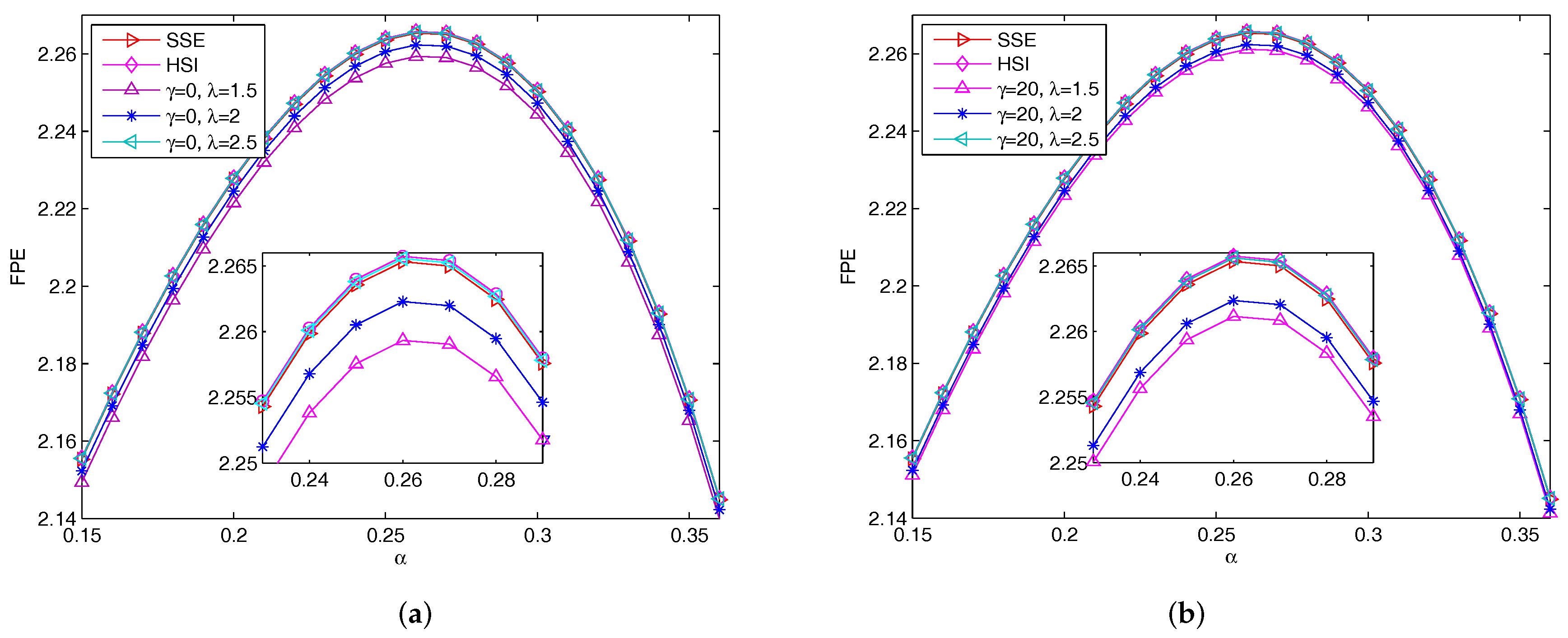
Figure 3.
FSE versus for the actual market datasets and the simulation ones: (a) For and . (b) For and . (c) For and . (d) For and . (e) For and . (f) For and .
Figure 3.
FSE versus for the actual market datasets and the simulation ones: (a) For and . (b) For and . (c) For and . (d) For and . (e) For and . (f) For and .


Table 1.
Descriptive statistics and tests of simulation datasets and actual datasets.
| Descriptive Statistics | K-S Test | A-D Test | ||||||||||||
| Mean | Std | Max | Min | Skewness | Kurtosis | ksstat | adstat | |||||||
| SSE | 0.0003 | 0.0171 | 0.0940 | −0.1044 | −0.3509 | 7.8473 | 0.0846 | 1 | 81.266 | 1 | ||||
| HSI | 0.0001 | 0.0155 | 0.1018 | −0.1099 | −0.2027 | 8.0296 | 0.0767 | 1 | 67.524 | 1 | ||||
| Mean | Std | Max | Min | Skewness | Kurtosis | ksstat | adstat | |||||||
| 0 | 1.5 | −0.0001 | 0.0080 | 0.0449 | −0.0539 | 0.0473 | 4.9788 | 0.0930 | 1 | 92.199 | 1 | |||
| 0 | 2 | −0.0001 | 0.0122 | 0.0617 | −0.0741 | −0.0767 | 5.9401 | 0.0690 | 1 | 65.553 | 1 | |||
| 0 | 2.5 | 0.0002 | 0.0170 | 0.0955 | −0.0917 | 0.0113 | 7.0522 | 0.0506 | 1 | 50.723 | 1 | |||
| 10 | 1.5 | −0.0001 | 0.0084 | 0.0702 | −0.0548 | 0.2197 | 5.2835 | 0.0900 | 1 | 90.403 | 1 | |||
| 10 | 2 | −0.0000 | 0.0126 | 0.0931 | −0.0751 | −0.0164 | 6.3699 | 0.0666 | 1 | 63.809 | 1 | |||
| 10 | 2.5 | 0.0003 | 0.0172 | 0.0955 | −0.1149 | −0.0326 | 8.1074 | 0.0494 | 1 | 47.488 | 1 | |||
| 20 | 1.5 | −0.0001 | 0.0089 | 0.0822 | −0.0691 | 0.2554 | 5.5807 | 0.0887 | 1 | 84.661 | 1 | |||
| 20 | 2 | −0.0001 | 0.0131 | 0.0916 | −0.0968 | −0.0472 | 7.0812 | 0.0652 | 1 | 60.104 | 1 | |||
| 20 | 2.5 | 0.0003 | 0.0176 | 0.1030 | −0.1143 | 0.0842 | 9.7433 | 0.0475 | 1 | 46.573 | 1 | |||
Table 2.
Permutation entropy of returns and absolute returns of simulation datasets and actual datasets.
Table 2.
Permutation entropy of returns and absolute returns of simulation datasets and actual datasets.
| SSE | 3.1679 | 3.1651 | 6.4748 | 6.4621 | 8.4739 | 8.4723 | ||||
| HSI | 3.1718 | 3.1701 | 6.4977 | 6.4758 | 8.4870 | 8.4813 | ||||
| 0 | 1.5 | 3.1684 | 3.1462 | 6.4735 | 6.4154 | 8.4732 | 8.4453 | |||
| 0 | 2 | 3.1723 | 3.1667 | 6.5032 | 6.4805 | 8.4858 | 8.4791 | |||
| 0 | 2.5 | 3.1768 | 3.1721 | 6.5088 | 6.4983 | 8.4900 | 8.4871 | |||
| 10 | 1.5 | 3.1701 | 3.1493 | 6.4803 | 6.4239 | 8.4740 | 8.4414 | |||
| 10 | 2 | 3.1725 | 3.1674 | 6.5047 | 6.4862 | 8.4857 | 8.4813 | |||
| 10 | 2.5 | 3.1765 | 3.1721 | 6.5104 | 6.4992 | 8.4896 | 8.4743 | |||
| 20 | 1.5 | 3.1695 | 3.1525 | 6.4784 | 6.4323 | 8.4795 | 8.4515 | |||
| 20 | 2 | 3.1738 | 3.1694 | 6.5069 | 6.4918 | 8.4964 | 8.4829 | |||
| 20 | 2.5 | 3.1770 | 3.1725 | 6.5150 | 6.4999 | 8.4986 | 8.4933 | |||
Table 3.
FPE of returns with different fractional exponent .
| 0 | |||||||||
| SSE | 2.2024 | 2.2276 | 2.2470 | 2.2599 | 2.2653 | 2.2625 | 2.2502 | 2.2274 | |
| HSI | 2.2028 | 2.2280 | 2.2474 | 2.2603 | 2.2657 | 2.2629 | 2.2506 | 2.2278 | |
| 0 | |||||||||
| 0 | 1.5 | 2.1964 | 2.2215 | 2.2409 | 2.2538 | 2.2593 | 2.2566 | 2.2445 | 2.2218 |
| 0 | 2 | 2.1994 | 2.2245 | 2.2439 | 2.2568 | 2.2623 | 2.2595 | 2.2473 | 2.2246 |
| 0 | 2.5 | 2.2026 | 2.2278 | 2.2472 | 2.2601 | 2.2656 | 2.2627 | 2.2505 | 2.2277 |
| 20 | 1.5 | 2.1982 | 2.2234 | 2.2428 | 2.2556 | 2.2611 | 2.2583 | 2.2462 | 2.2235 |
| 20 | 2 | 2.1994 | 2.2247 | 2.2443 | 2.2569 | 2.2625 | 2.2595 | 2.2475 | 2.2249 |
| 20 | 2.5 | 2.2027 | 2.2280 | 2.2474 | 2.2604 | 2.2658 | 2.2630 | 2.2509 | 2.2281 |
Table 4.
Smaple entropy of returns and absolute returns of simulation datasets and actual datasets.
| SSE | 2.1194 | 1.8067 | 2.0216 | 1.7344 | 1.9378 | 1.6509 | ||||
| HSI | 2.1302 | 1.8468 | 2.0744 | 1.7980 | 1.9929 | 1.7341 | ||||
| 0 | 1.5 | 1.9661 | 1.7812 | 1.8664 | 1.6724 | 1.7691 | 1.5854 | |||
| 0 | 2 | 2.1305 | 1.9127 | 2.0207 | 1.7799 | 1.8917 | 1.7286 | |||
| 0 | 2.5 | 2.2293 | 1.9970 | 2.1216 | 1.8878 | 2.0215 | 1.7942 | |||
| 10 | 1.5 | 1.9944 | 1.8212 | 1.9127 | 1.7277 | 1.8136 | 1.6510 | |||
| 10 | 2 | 2.1475 | 1.9497 | 2.0508 | 1.8215 | 1.9237 | 1.7310 | |||
| 10 | 2.5 | 2.2353 | 2.0116 | 2.1263 | 1.9040 | 2.0245 | 1.8116 | |||
| 20 | 1.5 | 2.0045 | 1.8383 | 1.9265 | 1.7443 | 1.8286 | 1.6781 | |||
| 20 | 2 | 2.1520 | 1.9604 | 2.0539 | 1.8329 | 1.9352 | 1.7729 | |||
| 20 | 2.5 | 2.2389 | 2.0169 | 2.1301 | 1.9052 | 2.0572 | 1.8246 | |||
Table 5.
FSE of returns with different exponent values .
| 0 | |||||||||
| SSE | 1.1101 | 1.5211 | 2.0227 | 2.6088 | 3.2493 | 3.8644 | 4.2683 | 4.0339 | |
| HSI | 1.1145 | 1.5351 | 2.0522 | 2.6615 | 3.3347 | 3.9923 | 4.4458 | 4.2561 | |
| Gaussian | 1.1349 | 1.6246 | 2.2593 | 3.0522 | 3.9930 | 5.0134 | 5.9105 | 6.1562 | |
| 0 | |||||||||
| 0 | 1.5 | 1.0947 | 1.4773 | 1.9338 | 2.4536 | 3.0026 | 3.5006 | 3.7712 | 3.4218 |
| 0 | 2 | 1.1100 | 1.5209 | 2.0222 | 2.6079 | 3.2478 | 3.8622 | 4.2652 | 4.0301 |
| 0 | 2.5 | 1.1181 | 1.5472 | 2.0783 | 2.7088 | 3.4119 | 4.1089 | 4.6088 | 4.4618 |
| 10 | 1.5 | 1.0997 | 1.4908 | 1.9607 | 2.4999 | 3.0754 | 3.6072 | 3.9155 | 3.5980 |
| 10 | 2 | 1.1126 | 1.5289 | 2.0391 | 2.6380 | 3.2965 | 3.9349 | 4.3660 | 4.1560 |
| 10 | 2.5 | 1.1184 | 1.5484 | 2.0809 | 2.7135 | 3.4196 | 4.1207 | 4.6253 | 4.4827 |
| 20 | 1.5 | 1.1011 | 1.4948 | 1.9687 | 2.5137 | 3.0974 | 3.6394 | 3.9594 | 3.6517 |
| 20 | 2 | 1.1128 | 1.5297 | 2.0408 | 2.6411 | 3.3015 | 3.9425 | 4.3764 | 4.1691 |
| 10 | 2.5 | 1.1187 | 1.5493 | 2.0830 | 2.7173 | 3.4259 | 4.1301 | 4.6386 | 4.4996 |
Table 6.
FSE of absolute returns with different exponent values .
| 0 | |||||||||
| SSE | 1.0785 | 1.4366 | 1.8557 | 2.3216 | 2.7982 | 3.2061 | 3.3773 | 2.9481 | |
| HSI | 1.0867 | 1.4566 | 1.8936 | 2.3852 | 2.8960 | 3.3463 | 3.5639 | 3.1712 | |
| Gaussian | 1.1349 | 1.6246 | 2.2593 | 3.0522 | 3.9930 | 5.0134 | 5.9105 | 6.1562 | |
| 0 | |||||||||
| 0 | 1.5 | 1.0698 | 1.4165 | 1.8182 | 2.2596 | 2.7039 | 3.0723 | 3.2011 | 2.7397 |
| 0 | 2 | 1.0844 | 1.4510 | 1.8829 | 2.3671 | 2.8681 | 3.3061 | 3.5102 | 3.1068 |
| 0 | 2.5 | 1.0971 | 1.4836 | 1.9463 | 2.4750 | 3.0362 | 3.5498 | 3.8376 | 3.5028 |
| 10 | 1.5 | 1.0776 | 1.4345 | 1.8517 | 2.3149 | 2.7880 | 3.1916 | 3.3581 | 2.9254 |
| 10 | 2 | 1.0895 | 1.4638 | 1.9075 | 2.4087 | 2.9325 | 3.3990 | 3.6343 | 3.2561 |
| 10 | 1.5 | 1.0988 | 1.4883 | 1.9557 | 2.4912 | 3.0617 | 3.5870 | 3.8882 | 3.5645 |
| 20 | 1.5 | 1.0798 | 1.4398 | 1.8616 | 2.3315 | 2.8133 | 3.2277 | 3.4060 | 2.9823 |
| 20 | 2 | 1.0909 | 1.4673 | 1.9142 | 2.4201 | 2.9503 | 3.4247 | 3.6689 | 3.2978 |
| 20 | 2.5 | 1.0989 | 1.4886 | 1.9564 | 2.4924 | 3.0636 | 3.5899 | 3.8920 | 3.5692 |
© 2017 by the authors. Licensee MDPI, Basel, Switzerland. This article is an open access article distributed under the terms and conditions of the Creative Commons Attribution (CC BY) license (http://creativecommons.org/licenses/by/4.0/).
Share and Cite
MDPI and ACS Style
Wang, Y.; Zheng, S.; Zhang, W.; Wang, J. Complex and Entropy of Fluctuations of Agent-Based Interacting Financial Dynamics with Random Jump. Entropy 2017, 19, 512. https://doi.org/10.3390/e19100512
AMA Style
Wang Y, Zheng S, Zhang W, Wang J. Complex and Entropy of Fluctuations of Agent-Based Interacting Financial Dynamics with Random Jump. Entropy. 2017; 19(10):512. https://doi.org/10.3390/e19100512
Chicago/Turabian StyleWang, Yiduan, Shenzhou Zheng, Wei Zhang, and Jun Wang. 2017. "Complex and Entropy of Fluctuations of Agent-Based Interacting Financial Dynamics with Random Jump" Entropy 19, no. 10: 512. https://doi.org/10.3390/e19100512
Note that from the first issue of 2016, this journal uses article numbers instead of page numbers. See further details here.