
Inferring Weighted Directed Association Networks from Multivariate Time Series with the Small-Shuffle Symbolic Transfer Entropy Spectrum Method

Abstract
:1. Introduction
1.1. Problem Statement
1.2. Related Works
1.3. Primary Contribution of This Work
- (1)
- Time series being non-stationary: the probabilities are estimated from observations of a single instance over a long time series. It is very important that the time series is statistically stationary over the period of interest, which can be a practical problem with transfer entropy calculations [38]. In most cases the time series from real industrial complex systems are non-stationary.
- (2)
- Time series being continuous: it is problematic to calculate the transfer entropy on continuous-valued time series. Thus, here we will resort to a solution.
- (3)
- Strong relationships identification: in general, when carrying out correlation analysis, we are more interested in strong correlations than weak correlations. Because the relationships among these variables are unknown, strong correlations are more convincing but weak correlations have a greater probability of misidentification and this may bring serious consequences. We don’t take the indirect correlation into account in the whole paper.
- (4)
- The direction and quantity of influence: the causality relation identification is crucial for network prediction and evolution. It is difficult to detect the directional influence that one variable exerts on another between two variables.
- (5)
- Temporal relation identification: we attempt to detect the specific temporal relation-based time lags, namely the function relation of time.
2. Methods
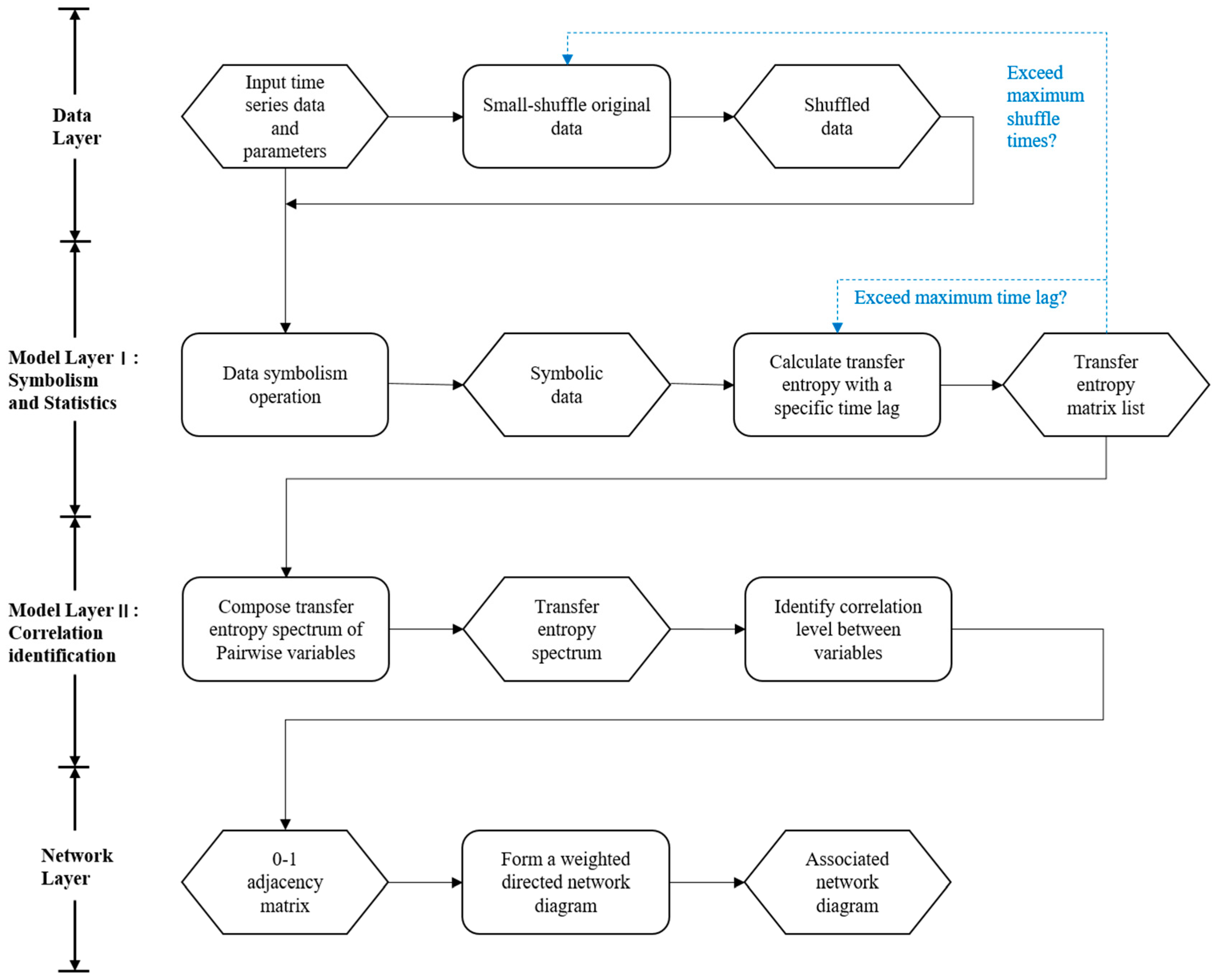
2.1. Main Principle
2.2. Small-Shuffle Surrogate Data Method
- (i)
- Shuffle the index of :where A is an amplitude.
- (ii)
- Sort by the rank order and let the index of be .
- (iii)
- Obtain the surrogate data:
2.3. Time Series Symbolization
2.4. Symbolic Transfer Entropy Calculation with Different Time Lags
| Algorithm 1: Symbolic Transfer Entropy Calculation with Different Time Lags |
| Input: STS, symbolic time series |
| tm, maximum time delay |
| Output: STEML, a list of symbolic transfer entropy matrix |
| Method: |
| for (t = 1; t <= tm; t++) { |
| colNum = column number of STS |
| for (i = 1; i <= colNum; j++) { |
| for (j = 1; j <= colNum; j++) { |
| if (j i) { |
| STS(j) = the column j of STS |
| STS(i) = the column i of STS |
| STE_matrix [i, j] = call_STE_Function(STS(j), STS(i), t) |
| } |
| } |
| } |
| Element t of STEML = STE_matrix |
| } |
| Return STEML |
2.5. Symbolic Transfer Entropy Spectrum Composition
2.6. Strong Correlation Identification
2.7. Association Network Inference
3. Results
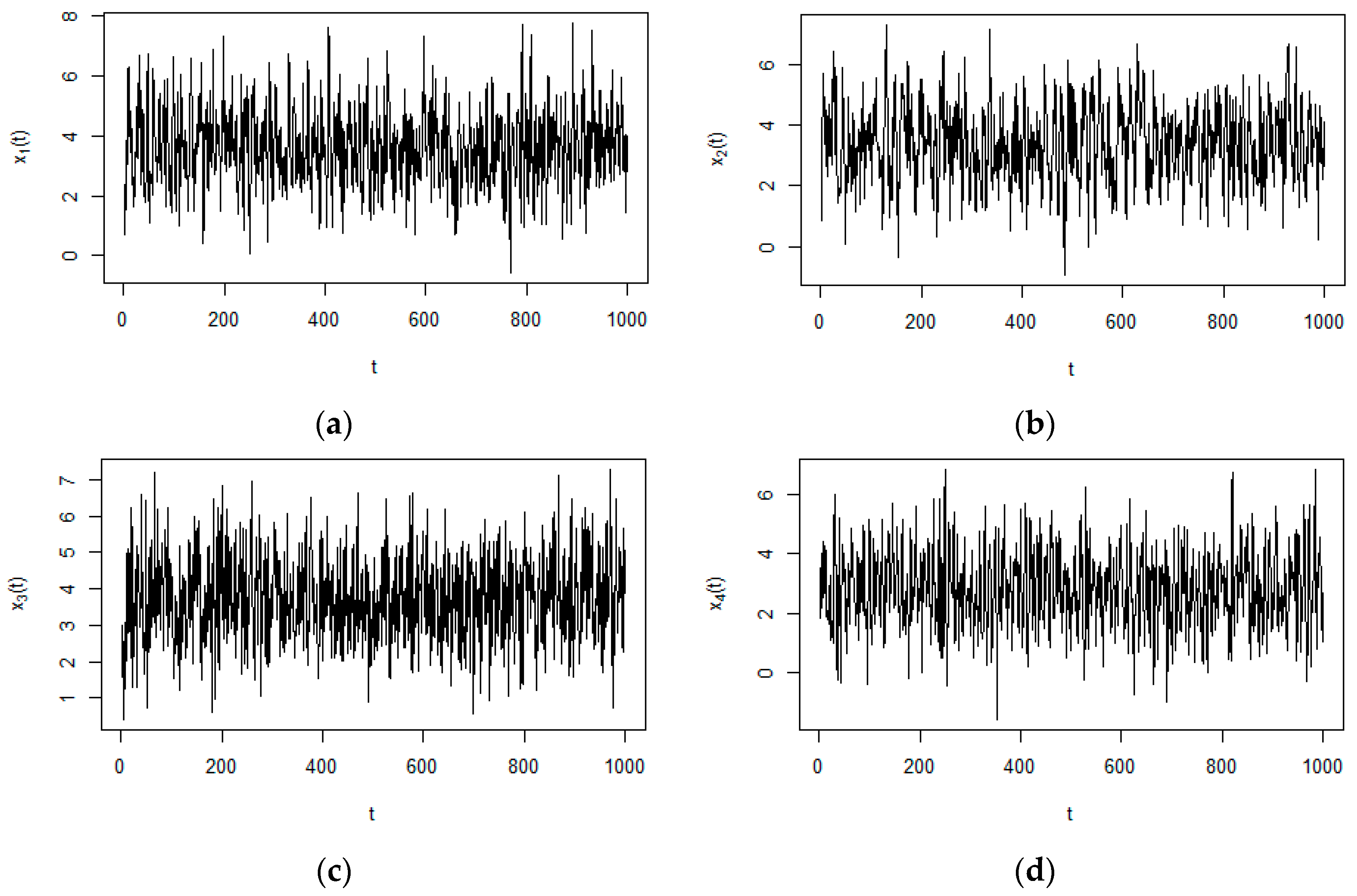
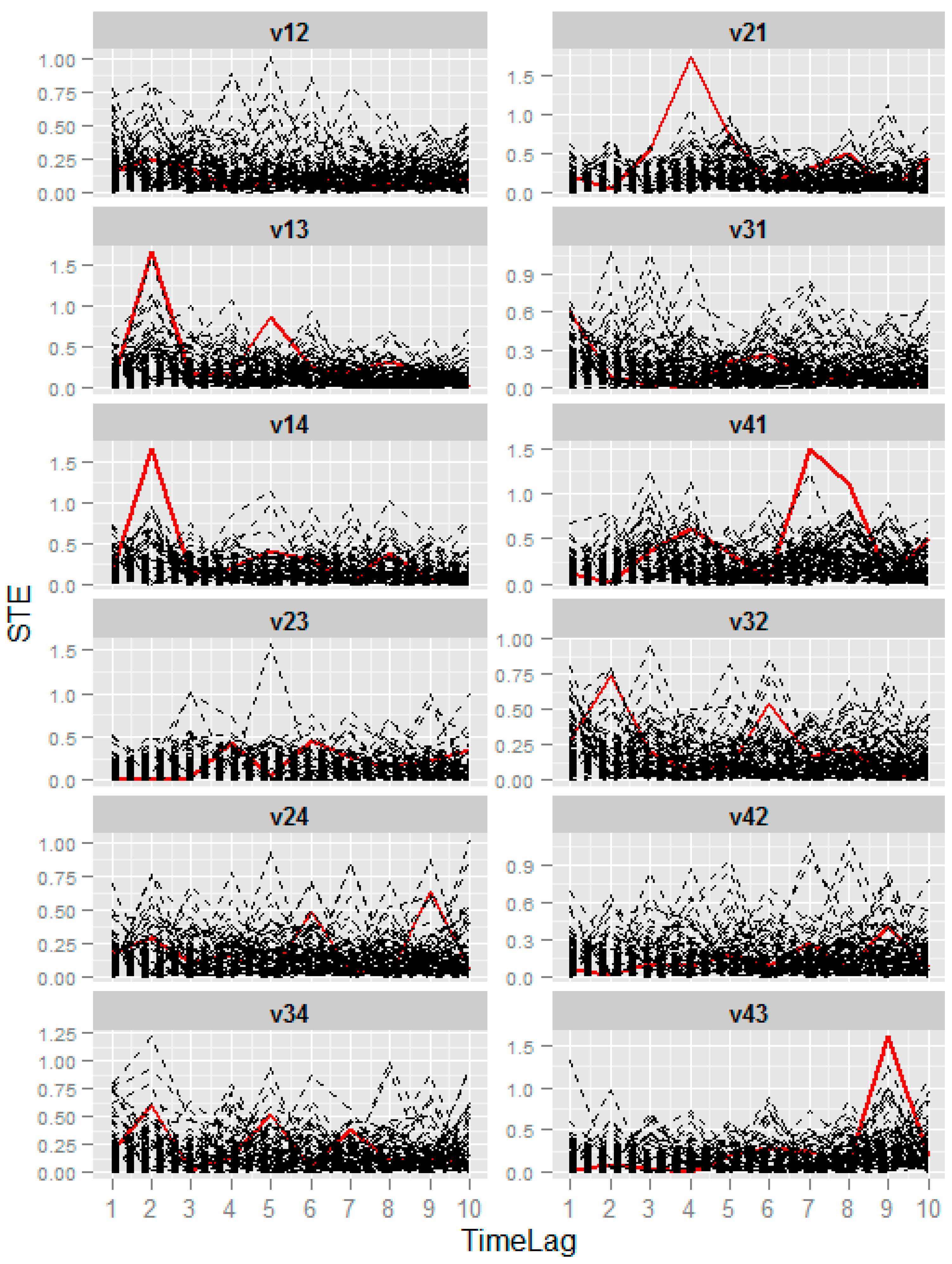
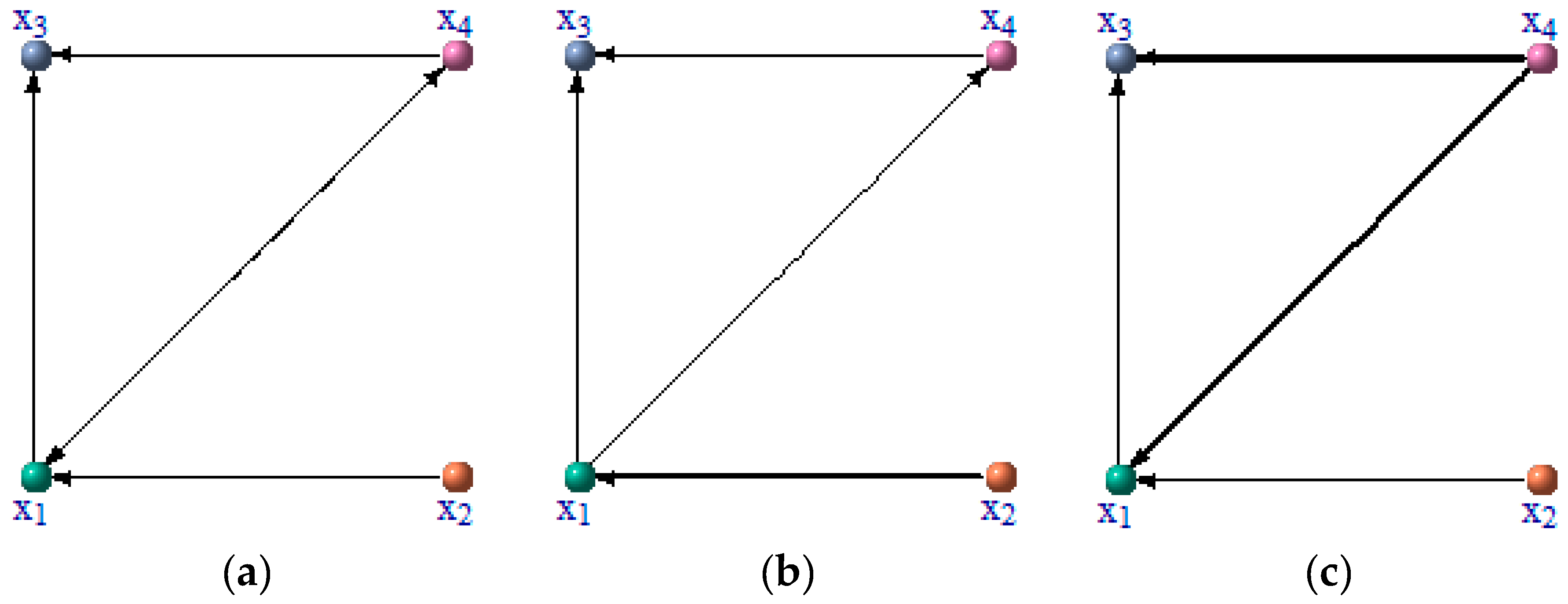
3.1. Numerical Example from Linear System
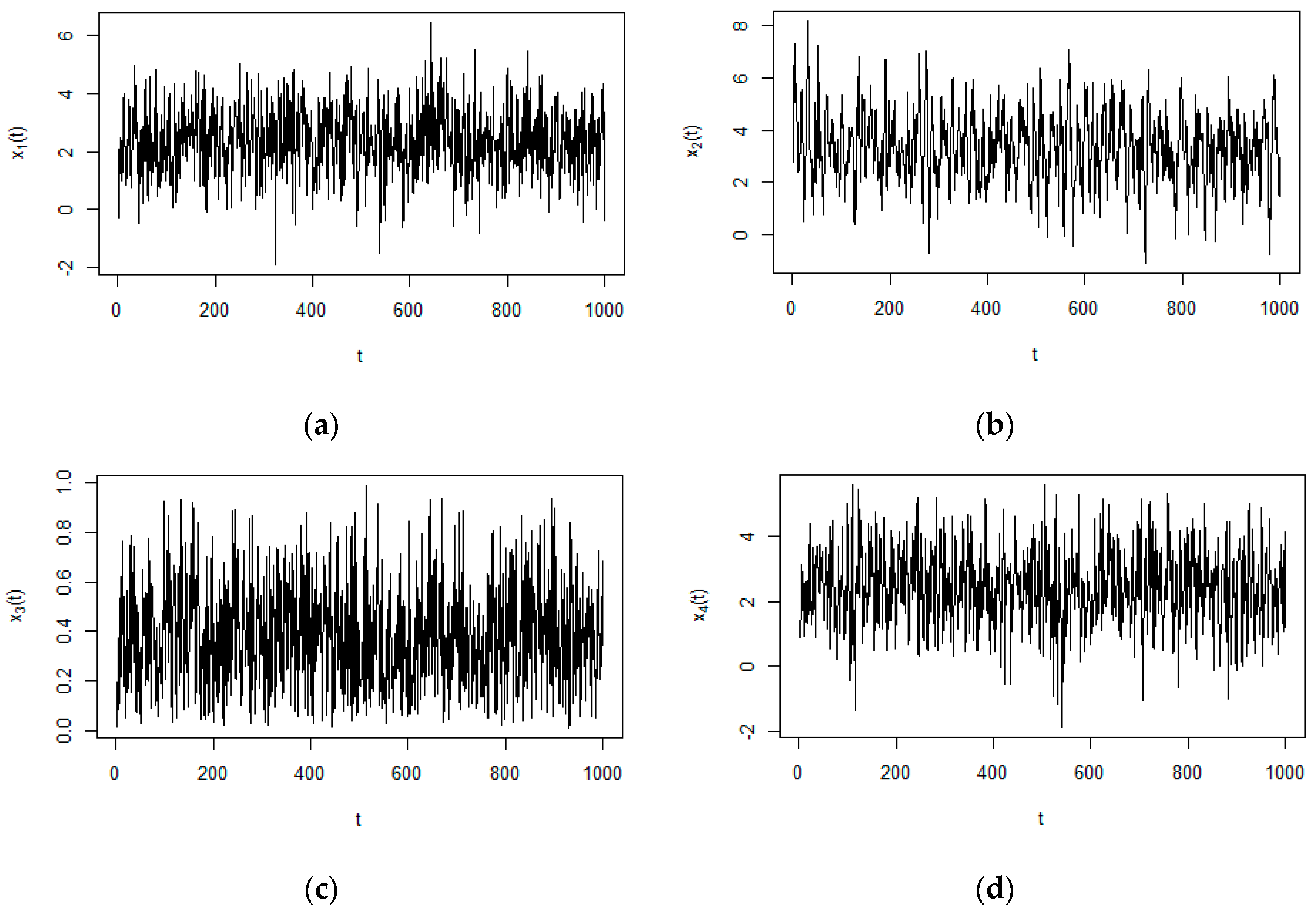
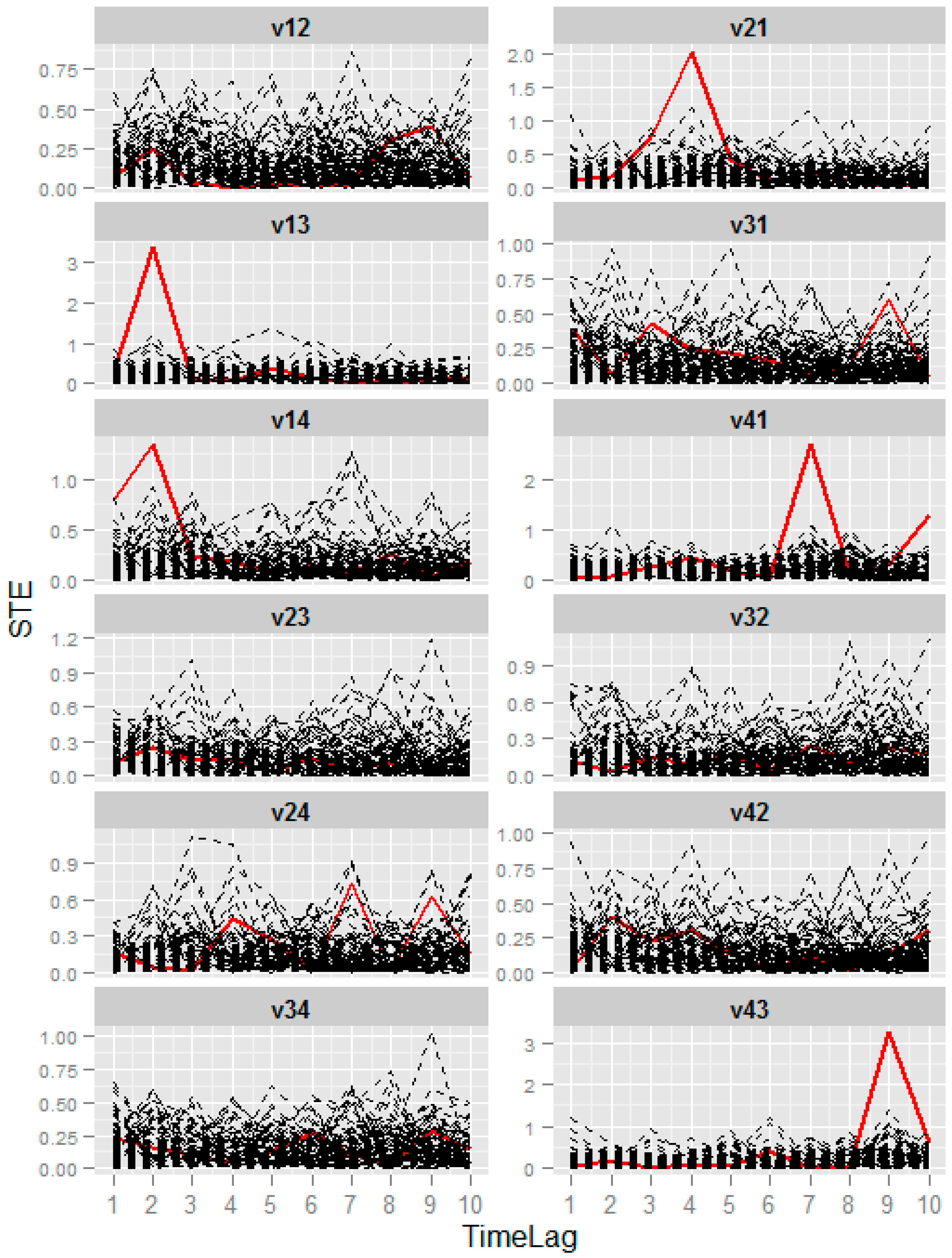
3.2. Numerical Example from Nonlinear System
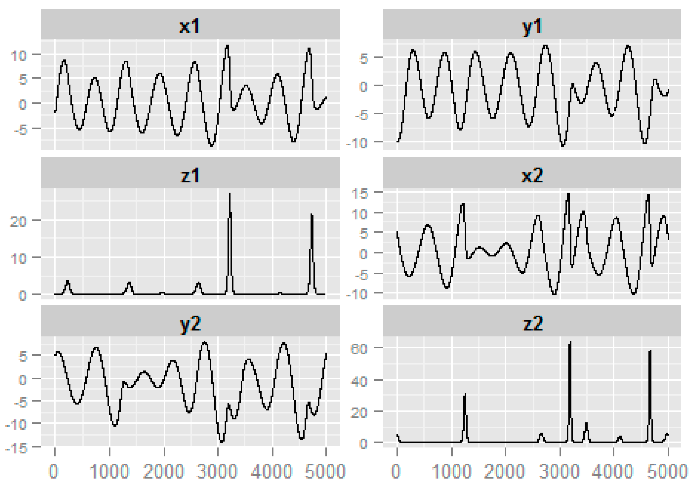
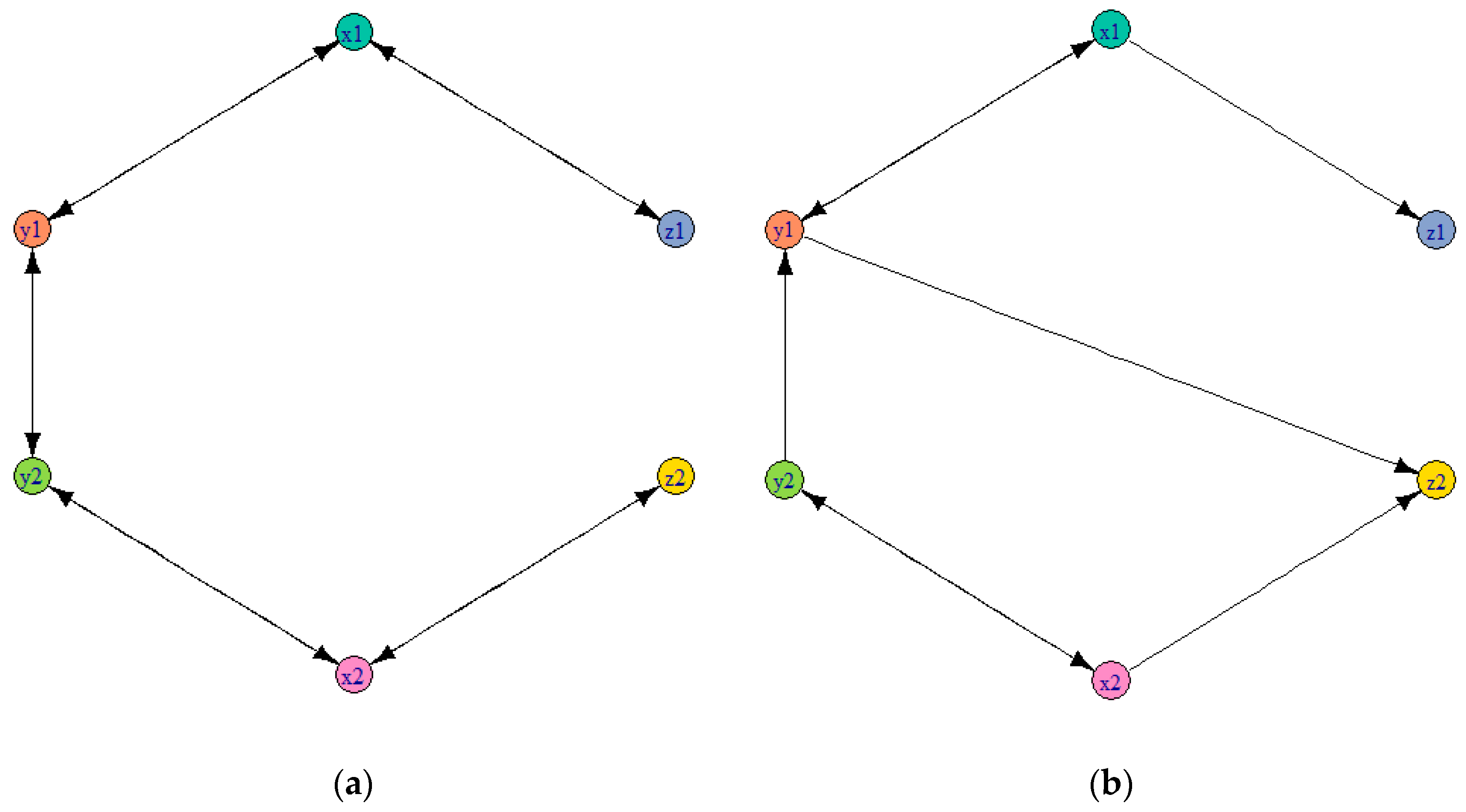
3.3. Numerical Example from the Coupled Rossler Systems
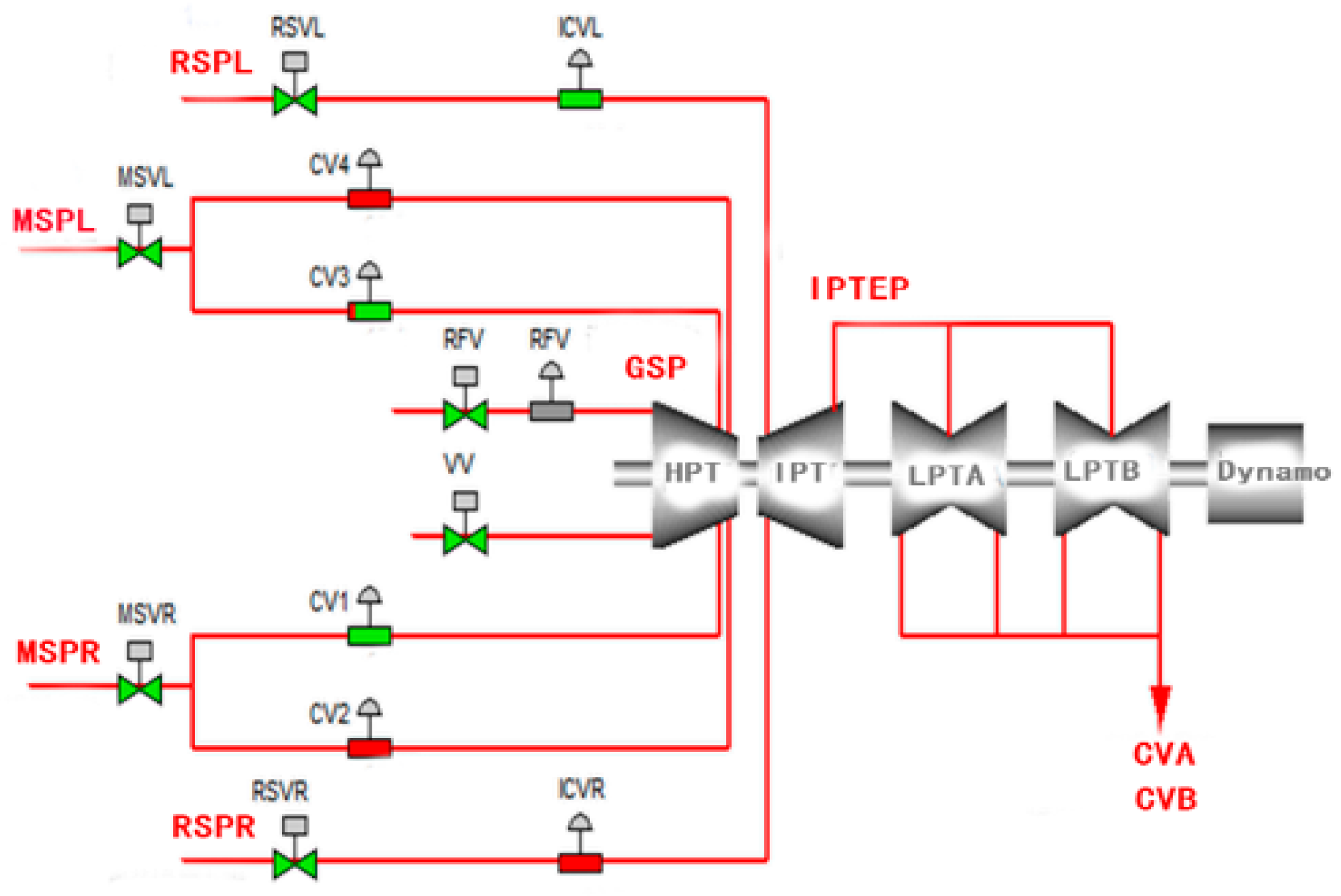
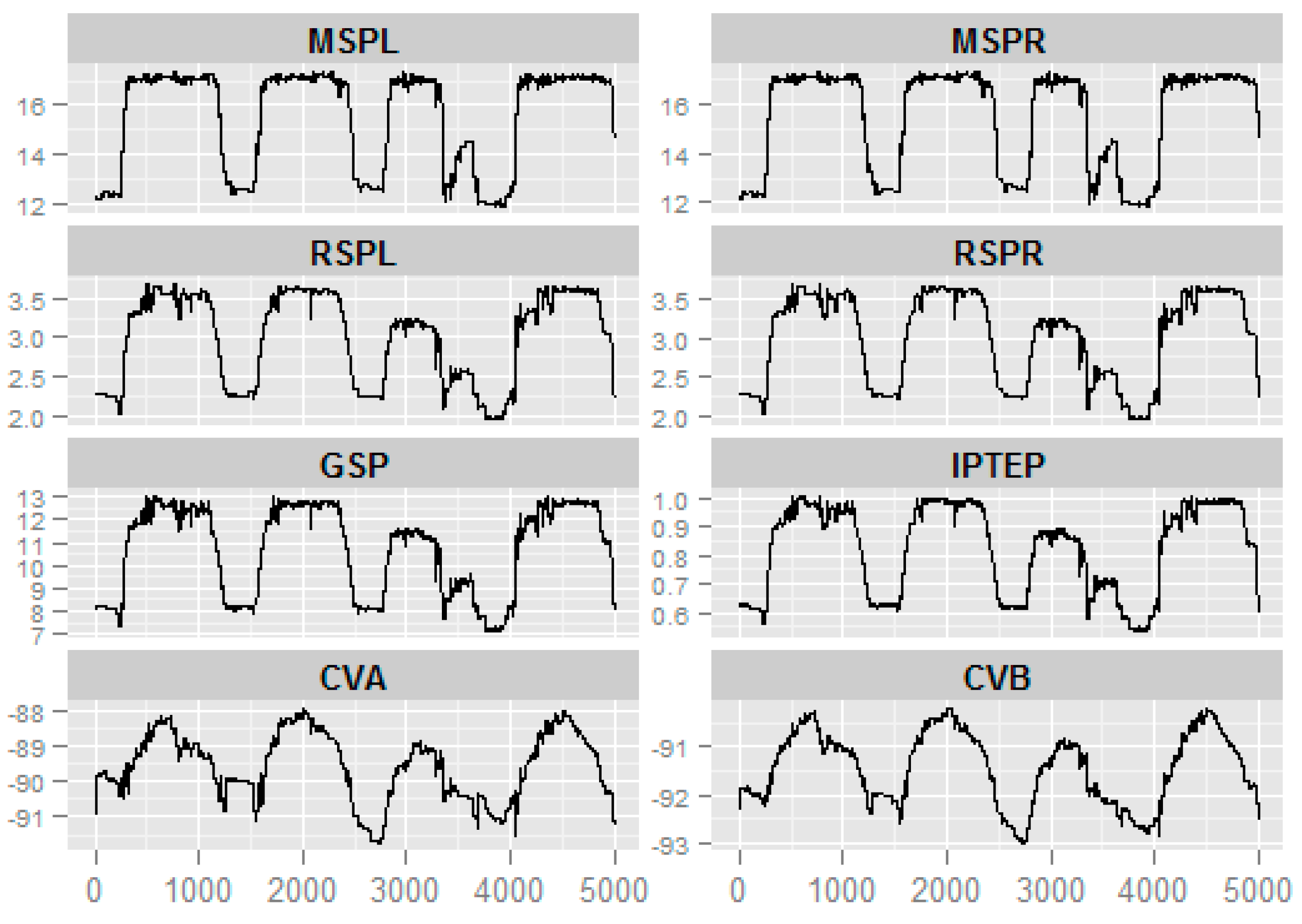
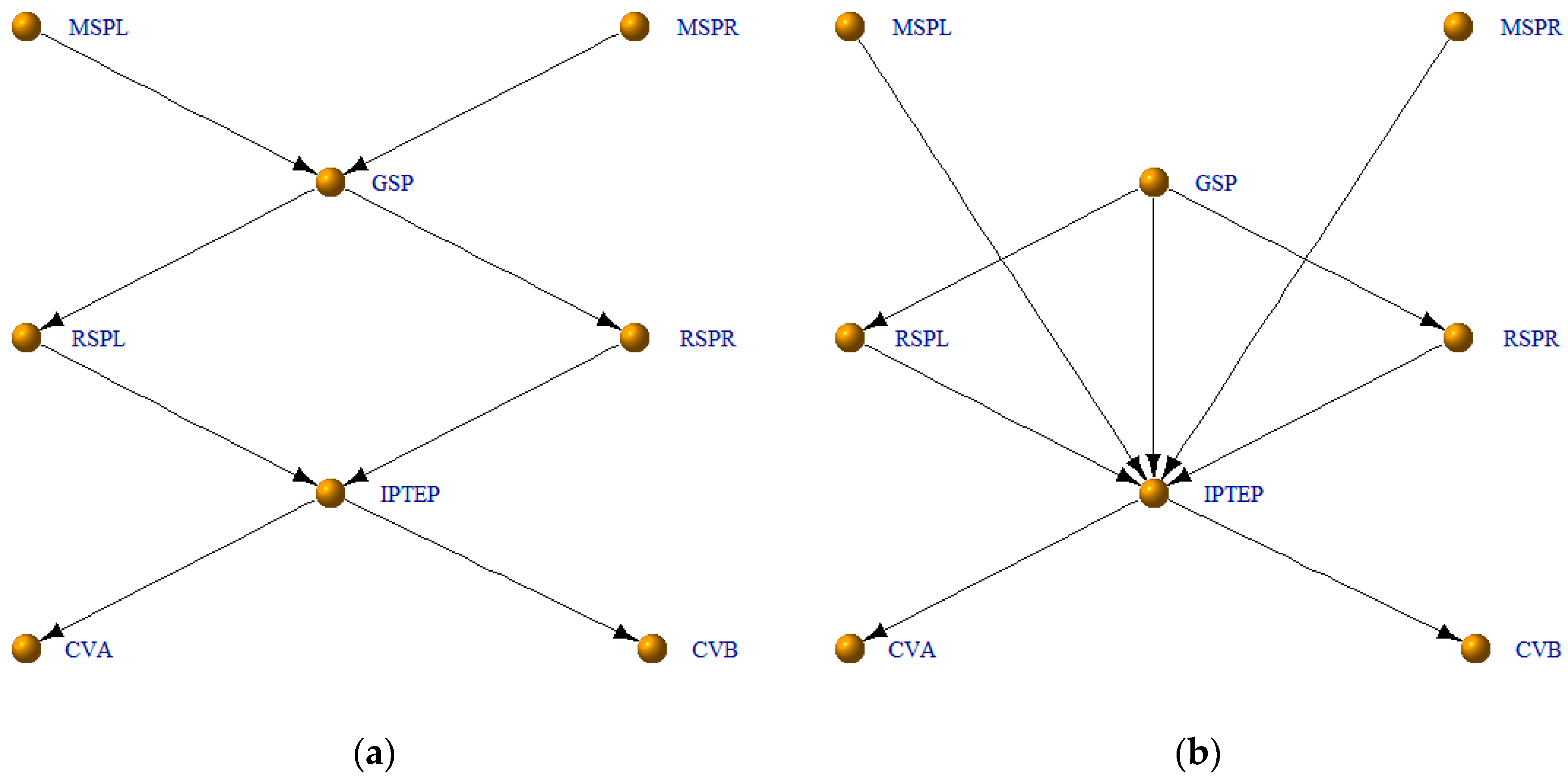
3.4. Application
4. Conclusions
Acknowledgments
Author Contributions
Conflicts of Interest
References
- De Solla Price, D.J. Networks of scientific papers. Science 1965, 149, 510–515. [Google Scholar] [CrossRef]
- Evans, T.S.; Hopkins, N.; Kaube, B.S. Universality of performance indicators based on citation and reference counts. Scientometrics 2012, 93, 473–495. [Google Scholar] [CrossRef] [Green Version]
- Goldberg, S.R.; Anthony, H.; Evans, T.S. Modelling citation networks. Scientometrics 2015, 105, 1577–1604. [Google Scholar] [CrossRef]
- Watts, D.J.; Strogatz, S.H. Collective dynamics of ‘small-world’ networks. Nature 1998, 393, 440–442. [Google Scholar] [CrossRef] [PubMed]
- Barabási, A.-L.; Albert, R. Emergence of scaling in random networks. Science 1999, 286, 509–512. [Google Scholar] [PubMed]
- Fernández-Rosales, I.Y.; Liebovitch, L.S.; Guzmán-Vargas, L. The dynamic consequences of cooperation and competition in small-world networks. PLoS ONE 2015, 10, e0126234. [Google Scholar] [CrossRef] [PubMed]
- Guo, X.; Zhang, Y.; Hu, W.; Tan, H.; Wang, X. Inferring nonlinear gene regulatory networks from gene expression data based on distance correlation. PLoS ONE 2014, 9, e87446. [Google Scholar] [CrossRef] [PubMed]
- Yuan, Y.; Li, C.-T.; Windram, O. Directed partial correlation: Inferring large-scale gene regulatory network through induced topology disruptions. PLoS ONE 2011, 6, e16835. [Google Scholar] [CrossRef] [PubMed]
- Cecchi, G.A.; Garg, R.; Rao, A.R. Inferring brain dynamics using granger causality on fmri data. In Proceedings of the 5th IEEE International Symposium on Biomedical Imaging, Paris, France, 14–17 May 2008. [CrossRef]
- Deng, L.; Sun, J.; Cheng, L.; Tong, S. Characterizing dynamic local functional connectivity in the human brain. Sci. Rep. 2016, 6, 26976. [Google Scholar] [CrossRef] [PubMed]
- Maucher, M.; Kracher, B.; Kühl, M.; Kestler, H.A. Inferring Boolean network structure via correlation. Bioinformatics 2011, 27, 1529–1536. [Google Scholar] [CrossRef] [PubMed]
- Han, L.; Zhu, J. Using matrix of thresholding partial correlation coefficients to infer regulatory network. Biosystems 2008, 91, 158–165. [Google Scholar] [CrossRef] [PubMed]
- Wang, Y.X.R.; Jiang, K.; Feldman, L.J.; Bickel, P.J.; Huang, H. Inferring gene-gene interactions and functional modules using sparse canonical correlation analysis. Ann. Appl. Stat. 2014, 9, 300–323. [Google Scholar] [CrossRef]
- Schäfer, J.; Strimmer, K. An empirical Bayes approach to inferring large-scale gene association networks. Bioinformatics 2005, 21, 754–764. [Google Scholar] [CrossRef] [PubMed]
- Huynh-Thu, V.A.; Irrthum, A.; Wehenkel, L.; Geurts, P. Inferring regulatory networks from expression data using tree-based methods. PLoS ONE 2010, 5, e12776. [Google Scholar] [CrossRef] [PubMed]
- Margolin, A.A.; Wang, K.; Lim, W.K.; Kustagi, M.; Nemenman, I.; Califano, A. Reverse engineering cellular networks. Nat. Protoc. 2006, 1, 662–671. [Google Scholar] [CrossRef] [PubMed]
- Faith, J.J.; Hayete, B.; Thaden, J.T.; Mogno, I.; Wierzbowski, J.; Cottarel, G.; Kasif, S.; Collins, J.J.; Gardner, T.S. Large-scale mapping and validation of Escherichia coli transcriptional regulation from a compendium of expression profiles. PLoS Biol. 2007, 5. [Google Scholar] [CrossRef] [PubMed]
- Zoppoli, P.; Morganella, S.; Ceccarelli, M. TimeDelay-ARACNE: Reverse engineering of gene networks from time-course data by an information theoretic approach. BMC Bioinform. 2010, 11. [Google Scholar] [CrossRef] [PubMed]
- Villaverde, A.; Ross, J.; Banga, J. Reverse engineering cellular networks with information theoretic methods. Cells 2013, 2, 306–329. [Google Scholar] [CrossRef] [PubMed]
- Aliferis, C.F.; Statnikov, A.; Tsamardinos, I.; Mani, S.; Koutsoukos, X.D. Local causal and markov blanket induction for causal discovery and feature selection for classification part I: Algorithms and empirical evaluation. J. Mach. Learn. Res. 2010, 11, 171–234. [Google Scholar]
- Dondelinger, F.; Husmeier, D.; Lèbre, S. Dynamic bayesian networks in molecular plant science: Inferring gene regulatory networks from multiple gene expression time series. Euphytica 2012, 183, 361–377. [Google Scholar] [CrossRef]
- En Chai, L.; Saberi Mohamad, M.; Deris, S.; Khim Chong, C.; Choon, Y.W.; Omatu, S. Current development and review of dynamic bayesian network-based methods for inferring gene regulatory networks from gene expression data. Curr. Bioinform. 2014, 9, 531–539. [Google Scholar] [CrossRef]
- Wiener, N.; Wiener, N. The theory of prediction. Mod. Math. Eng. 1956, 1, 125–139. [Google Scholar]
- Granger, C.W.J. Investigating causal relations by econometric models and cross-spectral methods. Econometrica 1969, 37, 424–438. [Google Scholar] [CrossRef]
- Tilghman, P.; Rosenbluth, D. Inferring wireless communications links and network topology from externals using granger causality. In MILCOM 2013—2013 IEEE Military Communications Conference; IEEE: Piscataway, NJ, USA, 2013; pp. 1284–1289. [Google Scholar]
- Schiatti, L.; Nollo, G.; Rossato, G.; Faes, L. Extended granger causality: A new tool to identify the structure of physiological networks. Physiol. Meas. 2015, 36. [Google Scholar] [CrossRef] [PubMed]
- Montalto, A.; Stramaglia, S.; Faes, L.; Tessitore, G.; Prevete, R.; Marinazzo, D. Neural networks with non-uniform embedding and explicit validation phase to assess granger causality. Neural Netw. 2015, 71, 159–171. [Google Scholar] [CrossRef] [PubMed] [Green Version]
- Mahdevar, G.; Nowzaridalini, A.; Sadeghi, M. Inferring gene correlation networks from transcription factor binding sites. Genes Genet. Syst. 2013, 88, 301–309. [Google Scholar] [CrossRef] [PubMed]
- Friedman, J.; Alm, E.J. Inferring correlation networks from genomic survey data. PLoS Comput. Biol. 2012, 8, e1002687. [Google Scholar] [CrossRef] [PubMed] [Green Version]
- Carmeli, C.; Knyazeva, M.G.; Innocenti, G.M.; de Feo, O. Assessment of EEG synchronization based on state-space analysis. Neuroimage 2005, 25, 339–354. [Google Scholar] [CrossRef] [PubMed]
- Walker, D.M.; Carmeli, C.; Pérez-Barbería, F.J.; Small, M.; Pérez-Fernández, E. Inferring networks from multivariate symbolic time series to unravel behavioural interactions among animals. Anim. Behav. 2010, 79, 351–359. [Google Scholar] [CrossRef]
- Reshef, D.N.; Reshef, Y.A.; Finucane, H.K.; Grossman, S.R.; McVean, G.; Turnbaugh, P.J.; Lander, E.S.; Mitzenmacher, M.; Sabeti, P.C. Detecting novel associations in large data sets. Science 2011, 334, 1518–1524. [Google Scholar] [CrossRef] [PubMed]
- Xia, L.C.; Ai, D.; Cram, J.; Fuhrman, J.A.; Sun, F. Efficient statistical significance approximation for local similarity analysis of high-throughput time series data. Bioinformatics 2013, 29, 230–237. [Google Scholar] [CrossRef] [PubMed]
- Ruan, Q.; Dutta, D.; Schwalbach, M.S.; Steele, J.A.; Fuhrman, J.A.; Sun, F. Local similarity analysis reveals unique associations among marine bacterioplankton species and environmental factors. Bioinformatics 2006, 22, 2532–2538. [Google Scholar] [CrossRef] [PubMed]
- Montalto, A.; Faes, L.; Marinazzo, D. Mute: A matlab toolbox to compare established and novel estimators of the multivariate transfer entropy. PLoS ONE 2014, 9. [Google Scholar] [CrossRef] [PubMed] [Green Version]
- Ai, X. Inferring a drive-response network from time series of topological measures in complex networks with transfer entropy. Entropy 2014, 16, 5753–5776. [Google Scholar] [CrossRef]
- Papana, A.; Kyrtsou, C.; Kugiumtzis, D.; Diks, C. Partial Symbolic Transfer Entropy; University of Amsterdam: Amsterdam, The Netherlands, 2013; pp. 13–16. [Google Scholar]
- Thorniley, J. An improved transfer entropy method for establishing causal effects in synchronizing oscillators. In ECAL 2011; MIT Press: Cambridge, MA, USA, 2011; pp. 797–804. [Google Scholar]
- Theiler, J.; Eubank, S.; Longtin, A.; Galdrikian, B.; Doyne Farmer, J. Testing for nonlinearity in time series: The method of surrogate data. Phys. D Nonlinear Phenom. 1992, 58, 77–94. [Google Scholar] [CrossRef]
- Small, M. Applied Nonlinear Time Series Analysis: Applications in Physics, Physiology and Finance; World Scientific: Singapore, 2005; p. 260. [Google Scholar]
- Nakamura, T.; Hirata, Y.; Small, M. Testing for correlation structures in short-term variabilities with long-term trends of multivariate time series. Phys. Rev. E 2006, 74, 041114. [Google Scholar] [CrossRef] [PubMed]
- Nakamura, T.; Tanizawa, T.; Small, M. Constructing networks from a dynamical system perspective for multivariate nonlinear time series. Phys. Rev. E 2016, 93, 032323. [Google Scholar] [CrossRef] [PubMed]
- Bandt, C.; Pompe, B. Permutation entropy: A natural complexity measure for time series. Phys. Rev. Lett. 2002, 88, 174102. [Google Scholar] [CrossRef] [PubMed]
- Staniek, M.; Lehnertz, K. Symbolic transfer entropy. Phys. Rev. Lett. 2008, 100, 158101. [Google Scholar] [CrossRef] [PubMed]
- Ma, H.; Aihara, K.; Chen, L. Detecting causality from nonlinear dynamics with short-term time series. Sci. Rep. 2014, 4. [Google Scholar] [CrossRef] [PubMed]
- Hill, S.M.; Heiser, L.M.; Cokelaer, T.; Unger, M.; Nesser, N.K.; Carlin, D.E.; Zhang, Y.; Sokolov, A.; Paull, E.O.; Wong, C.K.; et al. Inferring causal molecular networks: Empirical assessment through a community-based effort. Nat. Methods 2016, 13, 310–318. [Google Scholar] [CrossRef] [PubMed]
- Rapp, P.E.; Cellucci, C.J.; Watanabe, T.A.A.; Albano, A.M.; Schmah, T.I. Surrogate data pathologies and the false-positive rejection of the null hypothesis. Int. J. Bifurc. Chaos 2001, 11, 983–997. [Google Scholar] [CrossRef]
- Sims, C.A. Money, income, and causality. Am. Econ. Rev. 1972, 62, 540–552. [Google Scholar]


| ID | Precision | Sensitivity | PTL |
|---|---|---|---|
| 1 | 1.00 | 0.80 | 1.00 |
| 2 | 1.00 | 0.60 | 1.00 |
| 3 | 1.00 | 0.60 | 1.00 |
| 4 | 0.80 | 0.80 | 0.75 |
| 5 | 0.60 | 0.60 | 1.00 |
| 6 | 1.00 | 0.80 | 1.00 |
| 7 | 1.00 | 0.80 | 1.00 |
| 8 | 0.80 | 0.80 | 1.00 |
| 9 | 1.00 | 0.80 | 1.00 |
| 10 | 1.00 | 0.80 | 1.00 |
| Average | 0.92 | 0.74 | 0.98 |
| ID | Precision | Sensitivity | PTL |
|---|---|---|---|
| 1 | 0.75 | 0.60 | 1.00 |
| 2 | 1.00 | 0.80 | 1.00 |
| 3 | 0.80 | 0.80 | 1.00 |
| 4 | 1.00 | 0.80 | 1.00 |
| 5 | 1.00 | 0.80 | 1.00 |
| 6 | 1.00 | 0.40 | 1.00 |
| 7 | 1.00 | 0.80 | 1.00 |
| 8 | 0.67 | 0.80 | 0.75 |
| 9 | 0.80 | 0.80 | 1.00 |
| 10 | 1.00 | 0.60 | 1.00 |
| Average | 0.90 | 0.72 | 0.98 |
| ID | Precision | Sensitivity |
|---|---|---|
| 1 | 1.00 | 0.60 |
| 2 | 0.75 | 0.60 |
| 3 | 0.75 | 0.60 |
| 4 | 0.86 | 0.60 |
| 5 | 0.75 | 0.60 |
| 6 | 0.88 | 0.70 |
| 7 | 0.75 | 0.60 |
| 8 | 0.88 | 0.70 |
| 9 | 1.00 | 0.60 |
| 10 | 0.75 | 0.60 |
| Average | 0.84 | 0.62 |
| ID | Method | Precision | Sensitivity |
|---|---|---|---|
| 1 | SSSTES | 0.67 | 0.75 |
| 2 | RSSTE | 0.27 | 0.38 |
| 3 | GC | 0.17 | 1.00 |
© 2016 by the authors; licensee MDPI, Basel, Switzerland. This article is an open access article distributed under the terms and conditions of the Creative Commons Attribution (CC-BY) license (http://creativecommons.org/licenses/by/4.0/).
Share and Cite
Hu, Y.; Zhao, H.; Ai, X. Inferring Weighted Directed Association Networks from Multivariate Time Series with the Small-Shuffle Symbolic Transfer Entropy Spectrum Method. Entropy 2016, 18, 328. https://doi.org/10.3390/e18090328
Hu Y, Zhao H, Ai X. Inferring Weighted Directed Association Networks from Multivariate Time Series with the Small-Shuffle Symbolic Transfer Entropy Spectrum Method. Entropy. 2016; 18(9):328. https://doi.org/10.3390/e18090328
Chicago/Turabian StyleHu, Yanzhu, Huiyang Zhao, and Xinbo Ai. 2016. "Inferring Weighted Directed Association Networks from Multivariate Time Series with the Small-Shuffle Symbolic Transfer Entropy Spectrum Method" Entropy 18, no. 9: 328. https://doi.org/10.3390/e18090328