
Generalized Robustness of Contextuality


1
School of Mathematics and Information Science, Shaanxi Normal University, Xi’an 710062, China
2
School of Ethnic Nationalities Education, Shaanxi Normal University, Xi’an 710062, China
*
Author to whom correspondence should be addressed.
Entropy 2016, 18(9), 297; https://doi.org/10.3390/e18090297
Submission received: 16 May 2016
/
Revised: 4 August 2016
/
Accepted: 9 August 2016
/
Published: 1 September 2016
(This article belongs to the Special Issue Quantum Information 2016)
Abstract
:Motivated by the importance of contextuality and a work on the robustness of the entanglement of mixed quantum states, the robustness of contextuality (RoC) of an empirical model e against non-contextual noises was introduced and discussed in Science China Physics, Mechanics and Astronomy (59(4) and 59(9), 2016). Because noises are not always non-contextual, this paper introduces and discusses the generalized robustness of contextuality (GRoC) of an empirical model e against general noises. It is proven that if and only if e is non-contextual. This means that the quantity can be used to distinguish contextual empirical models from non-contextual ones. It is also shown that the function is convex on the set of all empirical models and continuous on the set of all no-signaling empirical models. For any two empirical models e and f such that the generalized relative robustness of e with respect to f is finite, a fascinating relationship between the GRoCs of e and f is proven, which reads . Lastly, for any n-cycle contextual box e, a relationship between the GRoC and the extent of violating the non-contextual inequalities is established.
1. Introduction
Contextuality is one of the most interesting manifestations of the quantumness of physical systems and manifests itself in the famous Kochen–Specker theorem [1], which states that for every quantum system belonging to a Hilbert space of dimension greater than two, irrespective of its actual state, there exists a finite set of measurements whose results cannot be assigned in a context-independent manner. It exhibits the strength of correlations that comes out of a quantum state when measured by compatible measurements and plays a central role in quantum communication and quantum computation. For example, quantum contextuality is related to quantum error correction [2], random access codes [3], quantum key distribution [4] and one-location quantum games [5]. The work in [6] proved that contextuality can supply the “magic” for quantum computation by establishing a remarkable equivalence between the onset of contextuality and the possibility of universal quantum computation via magic state distillation. An important and interesting question is how to quantify quantum contextuality. A huge effort is being put into quantifying quantum contextuality by the mutual information of contextuality, the relative entropy of contextuality and the cost of contextuality [7].
Contextuality is a basic and amazing quantum property, as well as entanglement [8,9]. Moreover, contextuality has been formulated in terms of “empirical models”, i.e., families of probability distributions [10]. Due to the importance of contextuality and motivated by a work on the robustness of entanglement of mixed quantum states against noise and jamming [11], we proposed and discussed recently in [12,13] the robustness of contextuality (RoC) and the contextuality cost of an empirical model e, where denotes the minimal amount of contextuality-free mixing needed to wipe out all contextuality of e and denotes the minimal amount of contextuality mixing needed to prepare e. The following conclusions have been proven: (i) an empirical model e is contextual if and only if ; (ii) the robustness of contextuality (RoC) is convex and un-increasing under a non-contextuality-preserving affine mapping; (iii) RoC is bounded and continuous on the set of all no-signaling empirical models; (iv) e is non-contextual if and only if ; and (v) e is strongly contextual if and only if . Furthermore, a relationship between and has been obtained. Lastly, we have computed and compared the RoCs of three empirical models. This means that the quantities and are measures for the contextuality of an empirical model e. However, noises are not always non-contextual. Motivated by a work on the generalized robustness of the entanglement of mixed quantum states against noise and jamming [14], in this paper, we consider the generalized robustness of contextuality (GRoC) , which characterizes the minimal amount of mixing with general noises (i.e., both non-contextual empirical models and contextual empirical models), which washes out all contextuality of e.
For any measurement scenarios, the problem of separating non-contextual from contextual correlations has been solved in [10,15]. In particular, Reference [16] provided the complete characterization of the non-contextual correlations for the case of dichotomic observables , where each consecutive pair , sum mod n, is jointly measurable. This generalizes both the Clauser–Horne–Shimony–Holt and the Klyachko–Can–Binicioglu–Shumovsky scenarios [17,18,19,20,21], which are the simplest ones for locality and non-contextuality, respectively. Such correlations can be formulated by an n-cycle box e [16], which is a family of probability distributions , where is a probability distribution on all possible outcomes of measurement . The contextuality of e can be completely characterized by the extent of violating the non-contextual inequalities in [16]. The work in [13] established the relationship between RoC and the violating of non-contextual inequalities for n-cycle boxes. Does there exist a relationship between the quantities and the extent of violating the non-contextual inequalities in [16]? In this paper, we will establish such a relationship.
This paper is organized as follows. In Section 2, we recall definitions and relevant results with respect to the contextuality of empirical models and the robustness of contextuality of empirical models and then introduce and observe the generalized robustness of contextuality (GRoC) , which characterizes the minimal amount of mixing with general noises (i.e., both non-contextual empirical models and contextual empirical models), which washes out all contextuality of e. Many properties of GRoC are proven, such as faithfulness, boundedness and continuity. It is worth noting that, for any two empirical models e and f, provided that the generalized relative robustness of e with respect to f is finite, i.e., there exists a finite non-negative number x, such that is non-contextual. In Section 3, by introducing a quantity representing the extent of violating the non-contextual inequalities in [16], we obtain the GRoC of any n-cycle boxes and can compare the robustness of contextuality against any noise for any n-cycle box and m-cycle one with .
2. Generalized Robustness of the Contextuality of Empirical Models
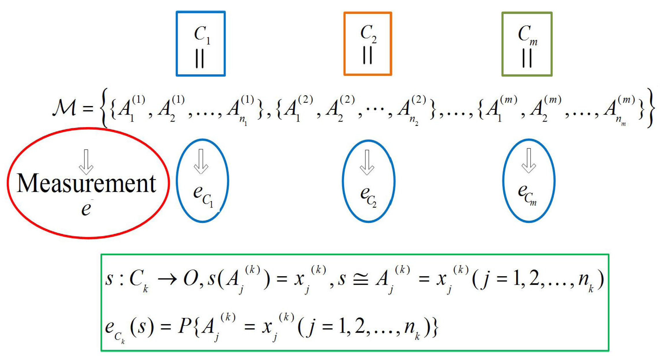
In [10], a measurement cover over a nonempty finite set X is defined as a family of nonempty subsets of X, such that and If in addition, O is a nonempty finite set, then the triple is said to be a measurement scenario (MS). In this case, the elements of X are called measurements; the ones of are called measurement contexts; and ones of O are called the outcomes of the measurements in X. The elements of the set consisting of all mappings are referred to as the events. Furthermore, we use to denote the set of all probability distributions over
Definition 1
([10]). Let be an MS. If for all , then the family is said to be an empirical model on .
Figure 1 is used to illustrate an empirical model: each context has a joint probability distribution under a measurement, such that is the probability that the event s with occurs.
Definition 2
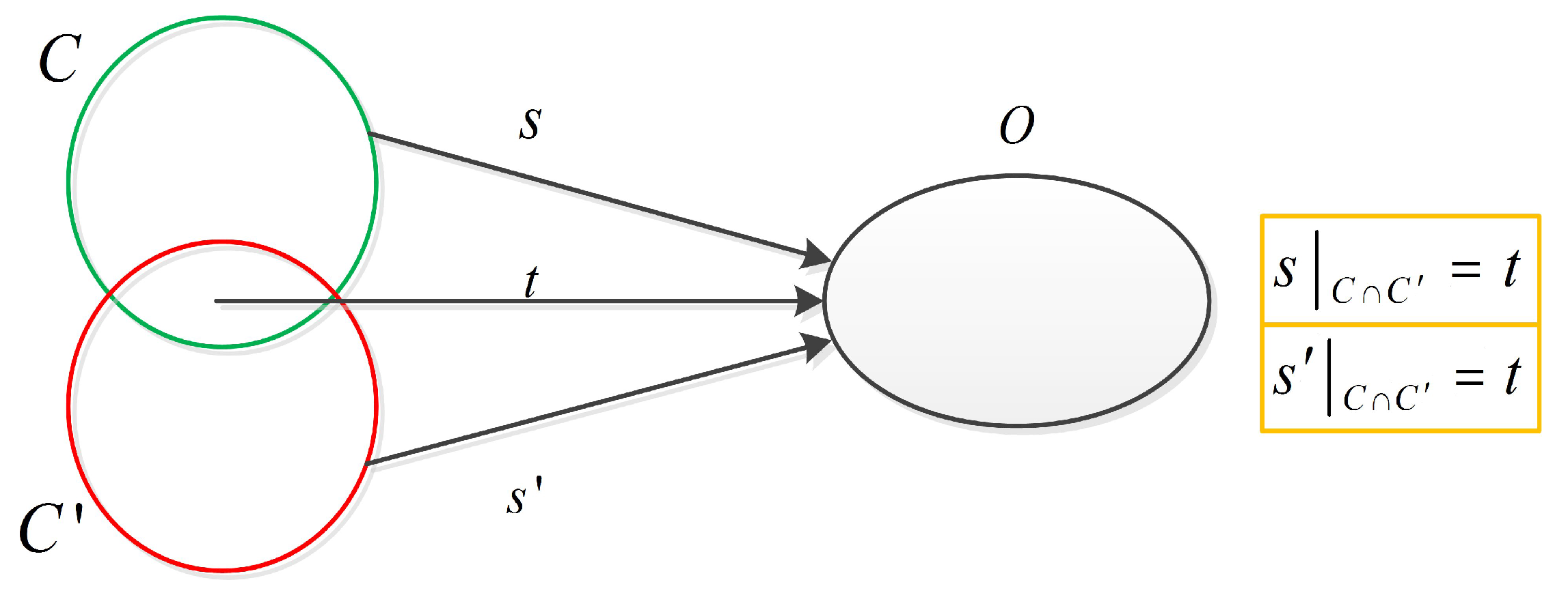
([10]). An empirical model on an MS is said to be a no-signaling empirical model if for all whenever with where:
For each event , the value of at t is defined as the sum of all values with , such that . Similarly, the value of at t is defined as the sum of all values with , such that . See Figure 2.
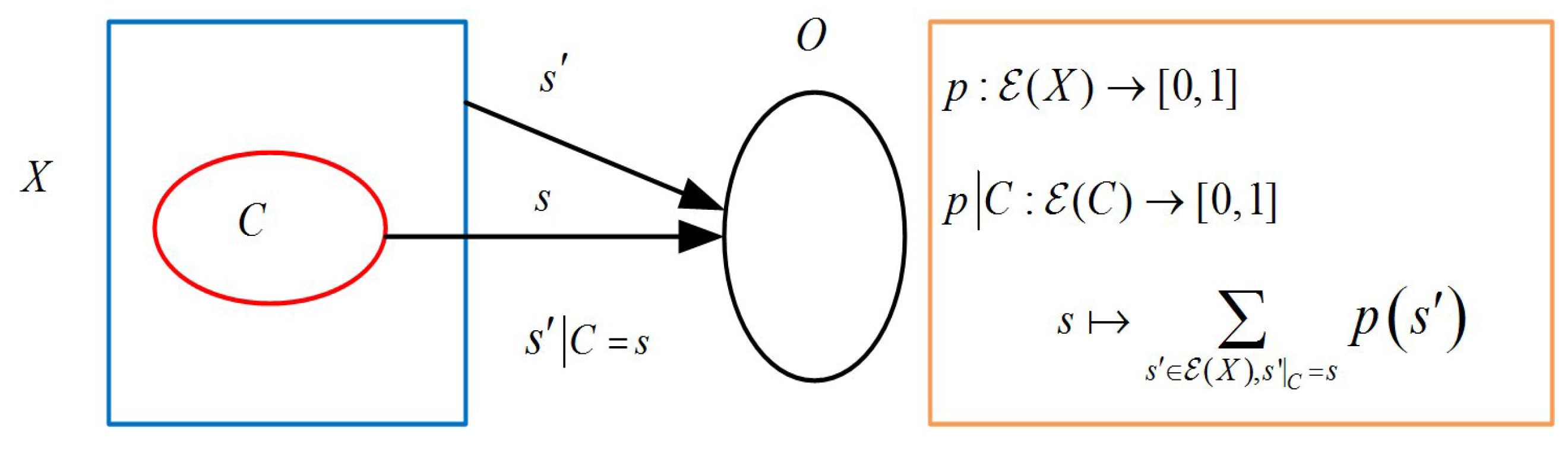
Let be an MS. Put:
For any and , we define:
and obtain , i.e., is a probability distribution for the measurements in context C.
Figure 3 illustrates the value of at , i.e., it is defined as the sum of all values with such that the restriction of on C is equal to s: .
Definition 3
([10]). An empirical model on an MS is said to be non-contextual if there exists such that for all Otherwise, it is said to be contextual.
Remark 1.
It is easy to check that every non-contextual empirical model is no-signaling.
In the following, we use and to denote the sets of all empirical models, no-signaling empirical models, non-contextual empirical models and contextual empirical models on an MS , respectively.
For any MS , put (the cardinality of the set ), and . Without loss of generality, we can write:
Definition 4
([10]). The incidence matrix associated with an MS given by (1) is defined as the ℓ by the matrix where if and ; and otherwise.
Definition 5
([10]). The incidence vector associated with empirical model on an MS given by Equation (1) is defined as the ℓ-dimensional column vector:
where if .
With these notations, the following theorems were proven in [10] (Proposition 4.1 and Theorem 5.5).
Theorem 1
([10]).
is non-contextual if and only if the equation has a non-negative real solution such that
Theorem 2
([10]).
For each , the linear system has a real solution such that
By looking carefully at the incidence matrix, we obtain the following theorem, which improves Theorem 1.
Theorem 3.
is non-contextual if and only if the equation has a non-negative real solution.
Proof.
Let be non-contextual. Then, we see from Theorem 1 that the equation has a non-negative real solution.
Let and the equation have a nonnegative real solution . Then:
By directly computing, we obtain that:
where the last equality holds since any entry of is either one or zero and the number of ones in every column of is m. Combining with Equation (3), we have . Therefore, the non-negative real solution to satisfies that . By Theorem 1, we obtain that e is non-contextual. □
By Theorem 3, only if the equation has a non-negative real solution, then e is non-contextual.
For given , put:
Due to the importance of contextuality and motivated by a work on the robustness of entanglement of mixed quantum states against noise and jamming [11], we have proposed and discussed the robustness of contextuality (RoC) of an empirical model e in [12,13] to quantify the amount of contextuality with respect to non-contextual mixing by asking about the minimal amount of contextuality-free mixing needed to wipe out all contextuality of e. The mathematical definition is as follows.
Definition 6
([12]). Let and . The relative robustness of contextuality of e with respect to is defined as:
and the robustness of contextuality (RoC) of e is defined as:
Contextual empirical model e is the object in which we are interested, and it is contextuality that supplies the “magic” for quantum computation. Although e is contextual, when it is mixed with a non-contextual empirical model , the mixture with may be non-contextual, and so, the contextuality of e is wiped out by . In this sense, we say that is noise or jamming. However, noises are not always non-contextual. Motivated by the generalized robustness [14] of entanglement, we investigate the generalized robustness of contextuality , which characterizes the minimal amount of mixing with general noises (i.e., both non-contextual empirical models and contextual ones), which washes out all contextuality of e.
Definition 7.
. The generalized relative robustness of contextuality of e with respect to is defined as:
and the generalized robustness of contextuality (GRoC) of e is defined as:
Considering that the minimums above are taken over compact sets and the functions to be optimized are continuous, we have that Equations (7) and (8) are well defined.
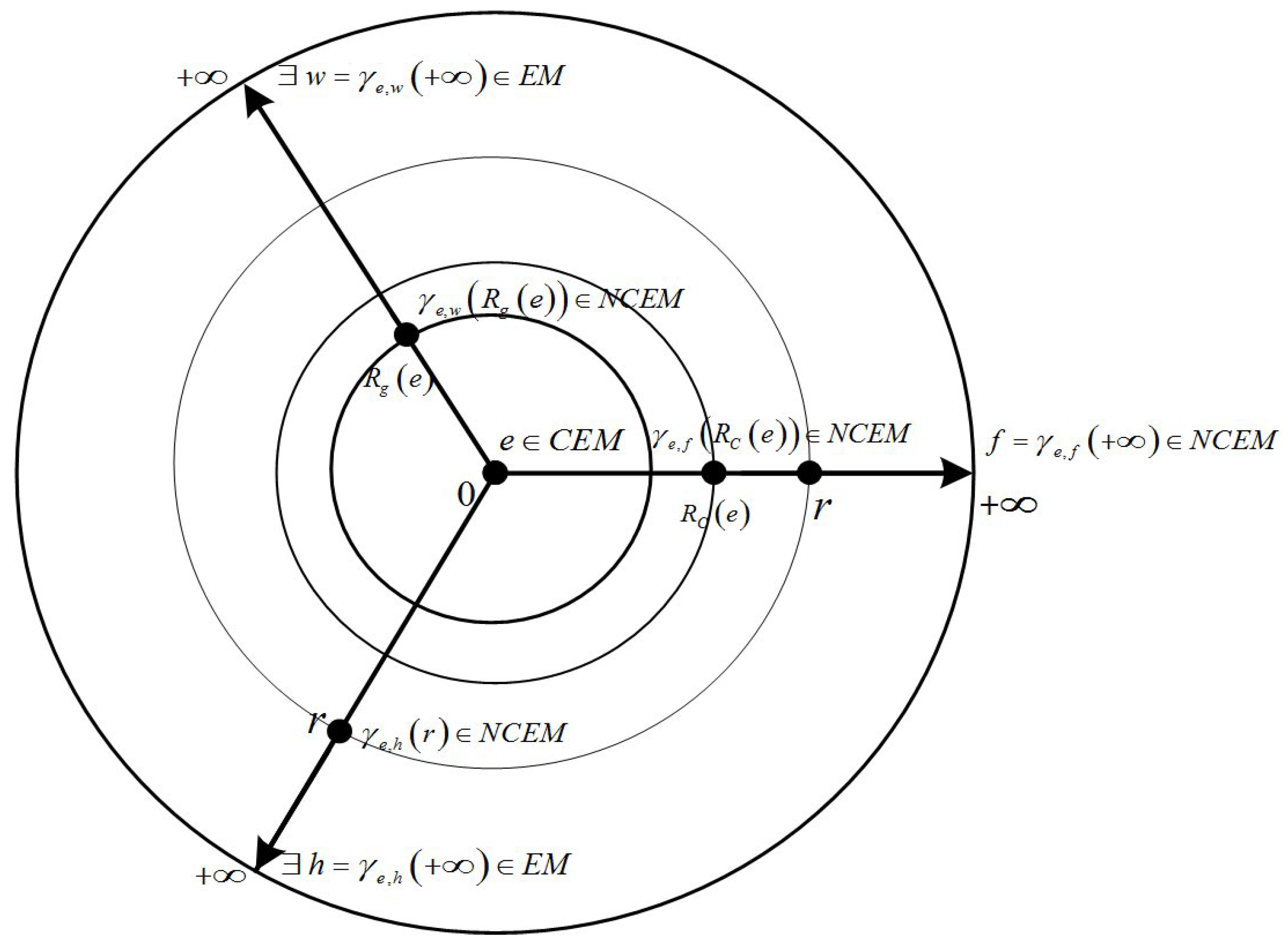
Figure 4 shows that implies that is contextual for all , and is non-contextual. In the case where , is non-contextual if and only if . Figure 5 shows that is finite, and the smallest radius of the circles containing non-contextual empirical models is . Moreover, the circle with radius contains non-contextual empirical models, and the circle with radius contains only contextual empirical models.
Remark 2.
By the definitions of RoC and GRoC of an empirical model e, we see that . For any , if , then is non-contextual, and so, by Remark 1. Thus, is the no-signaling since and
Using the norm-distance of in [12], a sequence in is convergent to e if and only if as for all . We see from [22] (Section 0.4.6) that there exist invertible matrices and and identity matrix such that:
For any positive integer n and , we denote:
Based on the above notations, the boundedness and continuity of GRoC on the set are proven in the following theorem. Moreover, the following theorem says that GRoC can be used to distinguish non-contextual empirical models from contextual ones.
Theorem 4.
(i) Let and be the empirical model , i.e., the totally mixed non-contextual empirical model. For any , it holds that:
(ii) is finite for any empirical model e; if and only if e is non-contextual.
(iii) For any , it holds that:
(iv) The GRoC function is convex on , i.e., if , then:
(v) for all with ; moreover, for any , there exists an empirical model f such that
(vi) as a function on is continuous, that is provided that such that .
Proof.
(i) Let . Theorem 2 implies that has a real solution . Put:
then:
Therefore, . Put then and so is a solution to with:
Let and be the empirical model . By directly computing, we obtain that . By Equation (14), we see that , and then:
Hence, is a non-negative solution to . Using Theorem 3, we obtain that is non-contextual. By Equation (7), we get that . Thus, we obtain by Equations (8) and (14) that Equation (11) holds.
(ii) First, let us prove that is finite for any empirical model e. To do this, we take an empirical model e and let given in (i). Note that for all , we can choose a small such that is an empirical model. Then, , and so, . This shows that Thus, is finite, even though it may be very large.
By the definitions of and , it is easy to know that for any . Since e is non-contextual if and only if , we obtain that for non-contextual . If , then there exists such that by Equations (7) and (8). Thus, .
(iii) Since e is contextual, we can assume that in the following. Put:
Then, , and so, is not empty.
At first, we shall show that is an upper bound of the set Suppose that there exists an such that Let for some such that where . For any , we see from the convexity of [12] that:
Set . Then:
which contradicts the property of . This shows that is an upper bound of the set
Then, we shall prove that is the supremum of the set Since e is contextual, we obtain from (ii) that . For any , take . Then, and . If there exists an such that , then , a contradiction. Hence, for all , and so, with . Therefore, , i.e., (12) holds.
(iv) Let:
and . Then by (ii) we see that both and are finite. Put Thus, there exist such that and:
Since and , we get and:
Observing that:
we see that . Consequently,
(v) Assume that . Clearly, if , then by Equation (8). We see from (ii) that , and so, . Next, we assume that . Then, . Since:
we obtain that and then:
For any , we see from Equation (8) that there exists an empirical model f such that . The first conclusion of (ii) yields that , and then, the first conclusion implies that .
(vi) Assume that such that . By the closedness of ([12], Theorem 2.2), we obtain that .
Claim 1.
Put Then, for some subsequence . For each there exists such that . The compactness of ([12], Theorem 2.2) yields that there exists a subsequence satisfying as . Since
and is closed, we have:
By Equation (7) and (8), we know that
Claim 2.
Assume that .
When the set is finite, then we obtain that .
When the set is infinite, there exists subsequence of such that for any j. For any , take:
Then:
Since and for any , we get that . For any , since and as j goes to infinity, we obtain that there exists positive integer such that:
Take:
Then, we have that for any , and . For any , take:
Thus, is convergent to zero since converges to e and for any j. Otherwise, when for some j, we have for any and . Since:
we obtain that for any , and then, , which contradicts the fact that for all j. Thus, we obtain a sequence of positive numbers with limit zero. Take:
for any . Since for any and , we have:
Hence,
and so, for any , we have that for all . By directly computing, we obtain that for any and then . Since:
is convex (by (iv)) and for any j (by (i)), we obtain that for any j,
Therefore,
Combining Claim 1 with Claim 2, we see that:
and then . □
By Equation (13), we observe that:
This means that there does not exist a parameter such that:
In other words, mixing of two empirical models does not increase simultaneously the GRoC of the mixed empirical models. Theorem 4. (v) says that and cannot be large simultaneously whenever and . By the compactness of ([12], Theorem 2.2), we obtain that Claim 1 also holds for such that , i.e. for any and any , there exists such that provided that with
Definition 8
([10]). An empirical model is said to be strongly contextual if for any there exists such that
Definition 9
([12]). The quantity:
is called the contextuality cost of .
Corollary 1.
There exists a strongly contextual such that:
Proof.
Since is continuous on and is a compact set, we obtain that has a maximal value on . For any , if e is not strongly contextual, then the cost of contextuality of e is strictly less than one ([12], Theorem 4.1), and there exist strongly contextual and non-contextual such that ([12], Corollary 4.1). Since h is non-contextual, we see from Theorem 4 that . It follows from the convexity of (Theorem 4) that:
This shows that the maximal value of over must be attained at some strongly contextual and no-signaling empirical model. □
3. The GRoC of -Cycle Boxes
In this section, we consider n dichotomic observables , where each consecutive pair , sum mod n, is jointly measurable and take:
Then, is an MS. The no-signaling empirical models on MS are said to be n-cycle boxes. To compute the GRoC of n-cycle boxes, the following notations and lemmas are needed. Denote events on measurement context as:
where the sum is mod n. Thus, for any . For any n-cycle box , take:
Put:
In the following, we assume that unless otherwise stated and compute .
Lemma 1
([16]). An n-cycle box e is non-contextual if and only if all tight non-contextuality inequalities hold, i.e.,
For an n-cycle box e, take:
Then, quantifies the extent of violating the non-contextual inequalities in Lemma 1. By Lemma 1 and Equation (17), we see that e is non-contextual if and only if .
Lemma 2.
For every contextual n-cycle box e, there exists one and only one non-contextuality inequality of all tight non-contextuality inequalities that is violated. That is, for an n-cycle box e, if there exists such that , then:
Proof.
Assume that such that . Let . Then, we obtain by Equation (16) that ; both and are odd numbers and . Therefore, there exist such that and . Since we obtain that by Equation (15). Moreover, since . Thus,
□
With these lemmas, we can prove the following theorem.
Theorem 5.
For any n-cycle box e, it holds that:
Proof.
- Case (i): If e is non-contextual, then we have that by Theorem 4 (ii) and for any by Lemma 1. By Equation (17), we see that , and so, (18) holds.
- Case (ii): If e is contextual, then there exists one and only one such that , and so:TakeThen, . Clearly, there exists n-cycle box f such that:
- Case (ii): If n is an even number, then we obtain that and . By Lemma 2, we have that:
Claim 3.
.
By Lemma 1 and Inequalities (19) and (20), we obtain that is non-contextual if and only if:
and:
i.e.,
By Equation (7), we obtain that .
Claim 4.
.
By Claim 3 and Equation (8), we have . Take:
and:
Then, .
For , we have:
Hence, we have from Lemma 1 that is contextual for any , and so, by Equation (7).
For , we have that , and so:
By Lemma 1 and Inequalities (19) and (21), we obtain that is non-contextual if and only if:
and:
i.e.,
Since:
for , we obtain that is non-contextual if and only if:
By Equation (7), we get that . Since , we see that .
When , we know that:
Combining Lemma 1 and Inequalities (19) and (23), we get that is non-contextual if and only if:
If , then for any , Inequality (24) is always violated, and so, is contextual. By Equation (7), we obtain from inequality (24) that . If , we obtain that is non-contextual if and only if:
By Equation (7), we see that:
Since , we obtain that .
When , there exists such that , and then:
By Lemma 1 and Inequalities (19) and (25), we have that is non-contextual if and only if:
and:
i.e.,
Hence,
Thus,
Since , we obtain that .
In a word, we obtain that for any and . Therefore, we have from Equation (8) that
- Case (ii): If n is an odd number, then it is easy to find that:
Claim 5.
.
From Lemma 1 and Inequalities (19) and (26), we get that is non-contextual if and only if
i.e.,
Therefore, .
Claim 6.
.
By Claim 5 and Equation (8), we have . Take:
For , it is easy to check that
For , we see from Lemma 1 and Inequality (18) that is non-contextual if and only if:
i.e.,
Hence,
For , there exists such that , and so:
By Lemma 1 and Inequalities (19) and (27), we obtain that is non-contextual if and only if:
and:
i.e.,
Hence,
Therefore,
Now, we have shown that for any . Therefore, . This shows that Equation (18) holds. □
Remark 3.
In [13], we have computed the robustness of contextuality of an n-cycle box e and obtained that:
Hence, for even n and for odd n.
Example 1.
For any n-cycle box f, we have for any i, and so, for any . Hence, by Equation (17), and then, Equation (18) implies that .
Let us consider the n-chain box in [7], which is given by:
By taking and , we obtain that and . Thus, by Equation (17), and then, Equation (18) implies that . This shows that:
4. Conclusions
Because noises are not always non-contextual, we have introduced and discussed the generalized robustness of contextuality (GRoC) of an empirical model e against general noises. We also have proven that if and only if e is non-contextual. This means that the quantity can be used to distinguish non-contextual empirical models from contextual ones. For any two empirical models e and f with , it has been proven , which reveals a fascinating relationship between the GRoCs of e and f. A relationship between GRoC and the extent of violating the non-contextual inequalities for n-cycle boxes has also been established, which reads . Thus, for any n-cycle boxes e and f, when , we have ; when e and f are contextual, we have if and only if . This means that can be used to quantify the contextuality of n-cycle boxes. Moreover, we have proven that the maximal value of over must be attained at some strongly contextual model. This shows that to some extent, contains the quantity of contextuality of e.
Acknowledgments
This work was supported by the National Natural Science Foundation of China (Grant Nos. 11371012, 11401359, 11471200, 11571211 and 11571213), the Fundamental Research Funds for the Central Universities (Grant No. GK201604001) and the Innovation Fund Project for Graduate Program of Shaanxi Normal University (Grant No. 2016CBY005).
Author Contributions
Wenhua Wang proved that the faithfulness of and Theorem 4(iii). Yajing Fan showed the convexity of . Liang Chen helped to depict the figures. The rest work of this paper was accomplished by Huaixin Cao and Huixian Meng, and discussed by the team of authors. All the authors have revised the paper carefully and approved the research contents that were written in the final manuscript. All authors have read and approved the final manuscript.
Conflicts of Interest
The authors declare no conflict of interest.
References
- Kochen, S.; Specker, E.P. The Problem of Hidden Variables in Quantum Mechanics. J. Math. Mech. 1967, 17, 59–87. [Google Scholar] [CrossRef]
- DiVincenzo, D.P.; Peres, A. Quantum code words contradict local realism. Phys. Rev. A 1997, 55, 4089–4092. [Google Scholar] [CrossRef]
- Galvão, E.F. Foundations of quantum theory and quantum information applications. Ph.D. Thesis, Oxford University, Oxford, UK, 2002. [Google Scholar]
- Nagata, K. Kochen-Specker theorem as a precondition for secure quantum key distribution. Phys. Rev. A 2005, 72, 012325. [Google Scholar] [CrossRef]
- Aharon, N.; Vaidman, L. Quantum advantages in classically defined tasks. Phys. Rev. A 2008, 77, 052310. [Google Scholar] [CrossRef]
- Howard, M.; Wallman, M.J.; Veitch, V.; Emerson, J. Contextuality supplies the “magic” for quantum computation. Nature 2014, 510, 351–355. [Google Scholar] [CrossRef] [PubMed]
- Grudka, A.; Horodecki, K.; Horodecki, M.; Horodecki, P.; Horodecki, R.; Joshi, P.; Klus, W.; Wocik, A. Quantifying contextuality. Phys. Rev. Lett. 2014, 112, 1204011. [Google Scholar] [CrossRef] [PubMed]
- Einstein, A.; Podolski, B.; Rosen, N. Can quantum-mechanical description of physical reality be considered complete? Phys. Rev. 1935, 47, 777. [Google Scholar] [CrossRef]
- Bell, J. Speakable and Unspeakable in Quantum Mechanics: Collected Papers on Quantum Philosophy; Cambridge University Press: Cambridge, UK, 1987. [Google Scholar]
- Abramsky, S.; Brandenburger, A. The Sheaf-theoretic structure of non-locality and contextuality. New J. Phys. 2011, 13, 113036. [Google Scholar] [CrossRef]
- Vidal, G.; Tarrach, R. Robustness of entanglement. Phys. Rev. A. 1999, 59, 141–155. [Google Scholar] [CrossRef] [Green Version]
- Meng, H.X.; Cao, H.X.; Wang, W.H. The robustness of contextuality and the contextuality cost of empirical models. Sci. China Phys. Mech. Astron. 2016, 59, 640303. [Google Scholar] [CrossRef]
- Meng, H.X.; Cao, H.X.; Wang, W.H.; Chen, L.; Fan, Y.J. Continuity of the robustness of contextuality of empirical models. Sci. China Phys. Mech. Astron. 2016, 59, 100311. [Google Scholar] [CrossRef]
- Steiner, M. Generalized robustness of entanglement. Phys. Rev. A. 2003, 67, 054305. [Google Scholar] [CrossRef]
- Abramsky, S.; Hardy, L. Logical Bell inequalities. Phys. Rev. A. 2012, 85, 062114. [Google Scholar] [CrossRef]
- Araújo, M.; Quintino, M.T.; Budroni, C.; Cunha, M.T.; Cabello, A. All non-contextuality inequalities for the n-cycle scenario. Phys. Rev. A. 2013, 88, 022118. [Google Scholar]
- Clauser, J.F.; Horne, M.A.; Shimony, A.; Holt, R.A. Proposed experiment to test Local Hidden-Variable theories. Phys. Rev. Lett. 1969, 23, 880. [Google Scholar] [CrossRef]
- Cabello, A. Experimentally testable state-independent quantum contextuality. Phys. Rev. Lett. 2008, 101, 210401. [Google Scholar] [CrossRef] [PubMed]
- Kirchmair, G.; Zahringer, F.; Gerritsma, R.; Kleinmann, M.; Guhne, O.; Cabello, A.; Blatt, R.; Roos, C.F. State-independent experimental test of quantum contextuality. Nature 2009, 460, 494–497. [Google Scholar] [CrossRef]
- Amselem, E.; Radmark, M.; Bourennane, M.; Cabello, A. State-independent quantum contextuality with single photons. Phys. Rev. Lett. 2009, 103, 160405. [Google Scholar] [CrossRef] [PubMed]
- Lapkiewicz, R.; Li, P.; Schaeff, C.; Langford, N.K.; Ramelow, S.; Wiesniak, M.; Zeilinger, A. An experimental proposal for revealing contextuality in almost all qutrit states. Sci. Rep. 2013, 3, 2706. [Google Scholar] [CrossRef]
- Horn, R.A.; Johnson, C.R. Matrix Analysis; Cambridge Univerisity Press: Cambridge, UK, 1985. [Google Scholar]
Figure 1.
An illustration of an empirical model.

Figure 2.
An illustration of and .

Figure 3.
An illustration of .

Figure 4.
An illustration of .
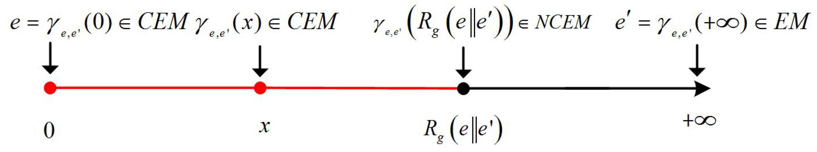
Figure 5.
An illustration of the GRoC of an empirical model e.

© 2016 by the authors; licensee MDPI, Basel, Switzerland. This article is an open access article distributed under the terms and conditions of the Creative Commons Attribution (CC-BY) license (http://creativecommons.org/licenses/by/4.0/).
Share and Cite
MDPI and ACS Style
Meng, H.; Cao, H.; Wang, W.; Fan, Y.; Chen, L. Generalized Robustness of Contextuality. Entropy 2016, 18, 297. https://doi.org/10.3390/e18090297
AMA Style
Meng H, Cao H, Wang W, Fan Y, Chen L. Generalized Robustness of Contextuality. Entropy. 2016; 18(9):297. https://doi.org/10.3390/e18090297
Chicago/Turabian StyleMeng, Huixian, Huaixin Cao, Wenhua Wang, Yajing Fan, and Liang Chen. 2016. "Generalized Robustness of Contextuality" Entropy 18, no. 9: 297. https://doi.org/10.3390/e18090297
Note that from the first issue of 2016, this journal uses article numbers instead of page numbers. See further details here.