
Greedy Algorithms for Optimal Distribution Approximation


Institute for Communications Engineering, Technical University of Munich, Munich 80290, Germany
*
Author to whom correspondence should be addressed.
Entropy 2016, 18(7), 262; https://doi.org/10.3390/e18070262
Submission received: 14 June 2016
/
Revised: 1 July 2016
/
Accepted: 11 July 2016
/
Published: 18 July 2016
(This article belongs to the Section Information Theory, Probability and Statistics)
Abstract
:The approximation of a discrete probability distribution by an M-type distribution is considered. The approximation error is measured by the informational divergence , which is an appropriate measure, e.g., in the context of data compression. Properties of the optimal approximation are derived and bounds on the approximation error are presented, which are asymptotically tight. A greedy algorithm is proposed that solves this M-type approximation problem optimally. Finally, it is shown that different instantiations of this algorithm minimize the informational divergence or the variational distance .

1. Introduction
In this work, we consider finite precision representations of probabilistic models. Suppose the original model, or target distribution, has n non-zero mass points and is given by . We wish to approximate it by a distribution of which each entry is a rational number with a fixed denominator. In other words, for every i, for some non-negative integer . The distribution is called an M-type distribution, and the positive integer is the precision of the approximation. The problem is non-trivial, since computing the numerator by rounding to the nearest integer in general fails to yield a distribution.
M-type approximations have many practical applications, e.g., in political apportionments, M seats in a parliament need to be distributed to n parties according to the result of some vote . This problem led, e.g., to the development of multiplier methods [1]. In communications engineering, example applications are finite precision implementations of probabilistic data compression [2], distribution matching [3], and finite-precision implementations of Bayesian networks [4,5]. In all of these applications, the M-type approximation should be close to the target distribution in the sense of an appropriate error measure. Common choices for this approximation error are the variational distance and the informational divergences:
where log denotes the natural logarithm.
Variational distance and informational divergence Equation (1b) have been considered by Reznik [6] and Böcherer [7], respectively, who presented algorithms for optimal M-type approximation and developed bounds on the approximation error. In a recent manuscript [8], we extended the existing works on Equation (1a,b) to target distributions with infinite support () and refined the bounds from [6,7].
In this work, we focus on the approximation error Equation (1c). It is an appropriate cost function for data compression [9] (Theorem 5.4.3) and seems appropriate for the approximation of parameters in Bayesian networks (see Section 4). Nevertheless, to the best of the authors’ knowledge, the characterization of M-type approximations minimizing has not received much attention in literature so far.
Our contributions are as follows. In Section 2, we present an efficient greedy algorithm to find M-type distributions minimizing Equation (1c). We then discuss in Section 3 the properties of the optimal M-type approximation and bound the approximation error Equation (1c). Our bound incorporates a reverse Pinsker inequality recently suggested in [10] (Theorem 7). The algorithm we present is an instance of a greedy algorithm similar to steepest ascent hill climbing [11] (Chapter 2.6). As a byproduct, we unify this work with [6,7,8] by showing that also the algorithms optimal w.r.t. variational distance Equation (1a) and informational divergence Equation (1b) are instances of the same general greedy algorithm, see Section 2.
2. Greedy Optimization
In this section, we define a class of problems that can be optimally solved by a greedy algorithm. Consider the following example:
Example 1.
Suppose there are n queues with jobs, and you have to select M jobs minimizing the total time spent. A greedy algorithm suggests to select successively the job with the shortest duration, among the jobs that are at the front of their queues. If the jobs in each queue are ordered by increasing duration, then this greedy algorithm is optimal.
We now make this precise: Let M be a positive integer, e.g., the number of jobs that have to be completed, and let , , be a set of functions, e.g., is the duration of the k-th job in the i-th queue. Let furthermore be a pre-allocation, representing a constraint that has to be fulfilled (e.g., in the i-th queue at least jobs have to be completed) or a chosen initialization. Then, the goal is to minimize
i.e., to find a final allocation satisfying and, for every i, . A greedy method to obtain such a final allocation is presented in Algorithm 1. We show in Appendix A.1. that this algorithm is optimal if the functions satisfy certain conditions:
| Algorithm 1: Greedy Algorithm |
| Initialize |
| repeat times |
| Compute |
| Compute // (choose one minimal element) Update |
| end repeat |
| Return c = (k1, ⋯, kn). |
Proposition 1.
If the functions are non-decreasing in k, Algorithm 1 achieves a global minimum for a given pre-allocation and a given M.
Remark 1.
The minimum of may not be unique.
Remark 2.
If a function is convex, the difference is non-decreasing in k. Hence, Algorithm 1 also minimizes
Remark 3.
Note that the functions need not be non-negative, i.e., in the view of Example 1, jobs may have negative duration. The functions are non-negative, though, if in Remark 2 is convex and non-decreasing.
Remark 2 connects Algorithm 1 to steepest ascent hill climbing [11] (Chapter 2.6) with fixed step size and a constrained number of M steps.
We now show that instances of Algorithm 1 can find M-type approximations minimizing each of the cost functions in Equation (1). Noting that for some non-negative integer , we can rewrite the cost functions as follows:
where denotes entropy in nats.
Ignoring constant terms, these cost functions are all instances of Remark 2 for convex functions (see Table 1). Hence, the three different M-type approximation problems set up by Equation (1) can all be solved by instances of Algorithm 1, for a trivial pre-allocation and after taking M steps. The final allocation simply defines the M-type approximation by .
For variational distance optimal approximation, we showed in [8] (Lemma 3), that every optimal M-type approximation satisfies , hence one may speed up the algorithm by pre-allocating . We furthermore show in Lemma 1 below that the support of the optimal M-type approximation in terms of Equation (1c) equals the support of (if ). Assuming that is positive, one can pre-allocate the algorithm with . We summarize these instantiations of Algorithm 1 in Table 1.
This list of instances of Algorithm 1 minimizing information-theoretic or probabilistic cost functions can be extended. For example, the -divergences and can also be minimized, since the functions inside the respective sums are convex. However, Rényi divergences of orders cannot be minimized by applying Algorithm 1.
3. -Type Approximation Minimizing
As shown in the previous section, Algorithm 1 presents a minimizer of the problem if instantiated according to Table 1. Let us call this minimizer . Recall that is positive and that . The support of must contain the support of , since otherwise . Note further that the costs are negative if and zero if ; hence, if , the index i cannot be chosen by Algorithm 1, thus also . This proves:
Lemma 1.
If , the supports of and coincide, i.e., .
The assumption that is positive and that hence comes without loss of generality. In contrast, neither variational distance nor informational divergence Equation (1b) require : As we show in [8], the M-type approximation problem remains interesting even if .
Based on Lemma 1, the following example explains why the optimal M-type approximation does not necessarily result in a “small” approximation error:
Example 2.
Let and , hence by Lemma 1, . It follows that , which can be made arbitrarily close to by choosing a small positive ε.
In Table 1 we made use of [8] (Lemma 3), which says that every minimizing the variational distance satisfies , to speed up the corresponding instance of Algorithm 1 by proper pre-allocation. Initialization by rounding is not possible when minimizing , as shown in the following two examples:
Example 3.
Let and . The optimal M-type approximation is , hence . Initialization via rounding off fails.
Example 4.
Let and . The optimal M-type approximation is , hence . Initialization via rounding up fails.
To show that informational divergence vanishes for , assume that for all i. Since the variational distance optimal approximation satisfies for every i, has the same support as , which ensures that . By similar arguments as in the proof of [8] (Proposition 4), we obtain
Note that this bound is universal, i.e., it prescribes the same convergence rate for every target distribution with n mass points.
We now develop an upper bound on that holds for every M. To this end, we first approximate by a distribution in that minimizes . If is unique, then it is called the reverse I-projection [12] (Section I.A) of onto . Since , its variational distance optimal approximation has the same support as , which allows us to bound by .
Lemma 2.
Let minimize . Then,
where is such that , and where .
Proof.
See Appendix A.2. ☐
Let , , and . The parameter must scale the mass such that it equals , i.e., we have
If, for all i, , then , hence is feasible and . One can show that decreases with M.
Proposition 2
(Approximation Bounds).
Proof.
See Appendix A.3. ☐
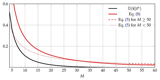
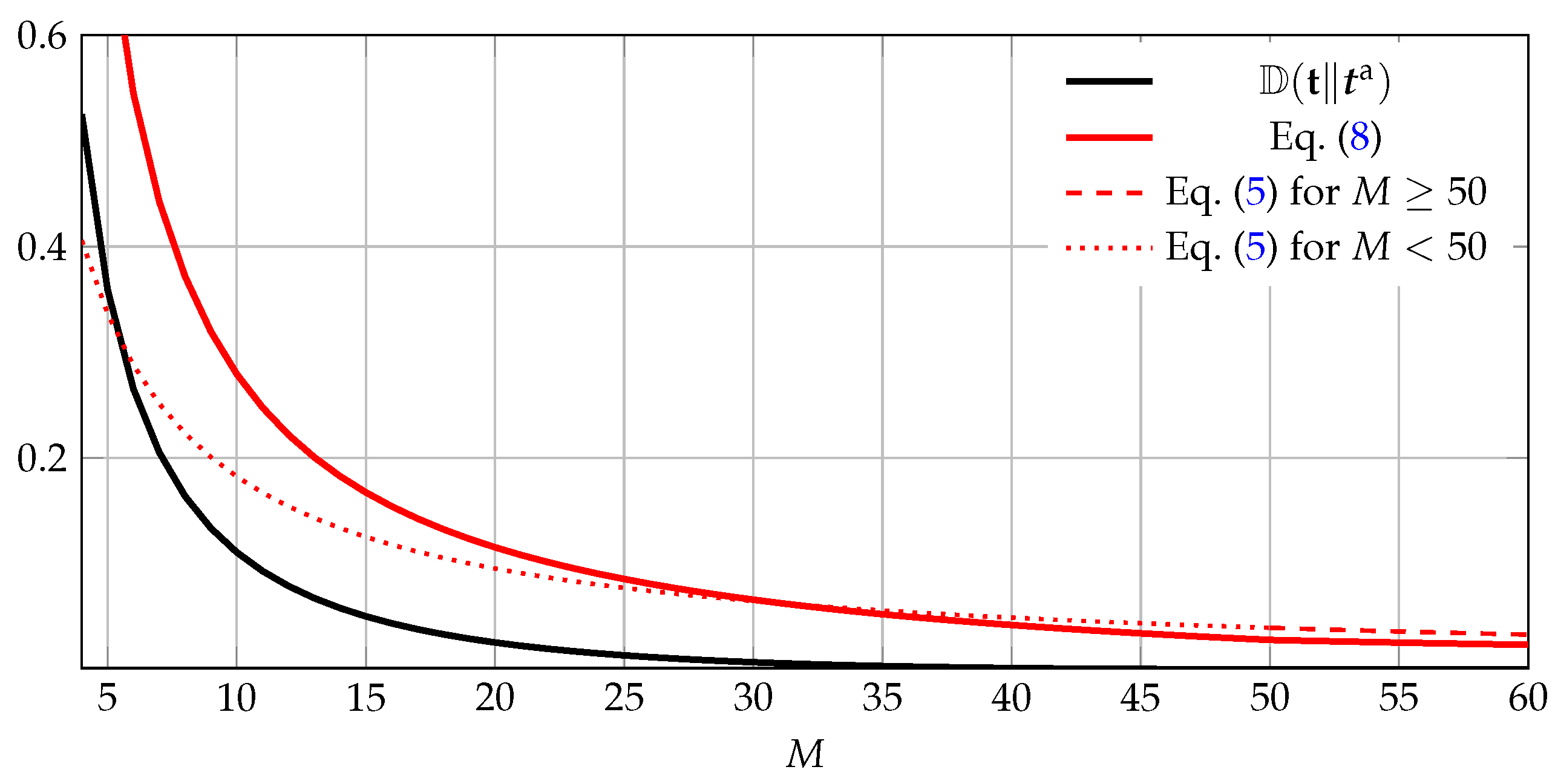
The first term on the right-hand side of Equation (8) accounts for the error caused by first approximating by (in the sense of Lemma 2). The second term accounts for the additional error caused by the M-type approximation of and incorporates the reverse Pinsker inequality [10] (Theorem 7). If for every i, hence , then and the bound simplifies to
For M sufficiently large, Equation (8) thus yields better results than Equation (5), which approximates to . Moreover, for M sufficiently large, our bound Equation (8) is uniform, i.e., it prescribes the same convergence rate for every target distribution with n mass points. We illustrate the bounds for an example in Figure 1.
4. Applications and Outlook
Arithmetic coding uses a probabilistic model to compress a source sequence. Applying Algorithm 1 with cost Equation (1c) to the empirical distribution of the source sequence provides an M-type distribution as a probabilistic model. The parameter M can be choosen small for reduced complexity. Another application of Algorithm 1 can be found in [3], which considers the problem of generating length-M sequences according to a desired distribution. Since a length-M sequence has an M-type empirical distribution, the Reference [3] applies Algorithm 1 with cost Equation () to pre-calculate the M-type approximation of the desired distribution.
Algorithm 1 can also be used to calculate the M-type approximation of Markov models, i.e., approximating the transition matrix of an n-state, irreducible Markov chain with invariant distribution vectors μ by a transition matrix containing only M-type probabilities. Generalizing Equation (1c), the approximation error can be measured by the informational divergence rate [13]
The optimal M-type approximation is found by applying the instance of Algorithm 1 to each row separately, and Lemma 1 ensures that the transition graph of equals that of , i.e., the approximating Markov chain is irreducible. Future work shall extend this analysis to hidden Markov models and should investigate the performance of these algorithms in practical scenarios, e.g., speech processing with finite-precision arithmetic.
Another possible application is the approximation of Bayesian network parameters. The authors of [4] approximated the true parameters using a stationary multiplier method from [14]. Since rounding probabilities to zero led to bad classification performance, they replaced zeros in the approximating distribution afterwards by small values. This in turn led to the problem that probabilities that are in fact zero, were approximated by a non-zero probability. We believe that these problems can be removed by instantiating Algorithm 1 for cost Equation (1c). This automatically prevents approximating non-zero probabilities with zeros and vice-versa, see Lemma 1.
Finally, for approximating Bayesian network parameters, recent work suggests rounding log-probabilities, i.e., to approximate by for a non-negative integer [5]. Finding an optimal approximation that corresponds to a true distribution is equivalent to solving
where denotes any of the considered cost functions Equation (1). If and using the binary logarithm, the constraint translates to the requirement that is approximated by a complete binary tree. Then, the optimal approximation is the Huffman code for .
Acknowledgments
The work of Bernhard C. Geiger was partially funded by the Erwin Schrödinger Fellowship J 3765 of the Austrian Science Fund. The work of Georg Böcherer was partly supported by the German Ministry of Education and Research in the framework of an Alexander von Humboldt Professorship. This work was supported by the German Research Foundation (DFG) and the Technical University of Munich (TUM) in the framework of the Open Access Publishing Program.
Author Contributions
Bernhard C. Geiger and Georg Böcherer conceived this study, derived the results, and wrote the manuscript. Specifically, Bernhard C. Geiger Proposition 1 and Lemmas 3, 5 and 6, and Georg Böcherer proved Lemmas 2 and 4. All authors have read and approved the final manuscript.
Conflicts of Interest
The authors declare no conflict of interest.
Appendix. Proofs
Appendix A.1. Proof of Proposition 1
Since a pre-allocation only fixes a lower bound for , w.l.o.g. we assume that and thus with . Consider the set and assume that the (not necessarily unique) set consists of M smallest values in , i.e., and
Clearly, cannot be smaller than the sum over all elements in . Since the are non-decreasing, there exists at least one final allocation that takes successively the first values from each queue i, i.e., satisfies Equation (A1). This shows that the lower bound induced by Equation (A1) can actually be achieved.
We prove the optimality of Algorithm 1 by contradiction: Assume that Algorithm 1 finishes with a final allocation such that is strictly larger than the (unique) sum over all elements in (non-unique) . Hence, must exchange at least one of the elements in for an element that is strictly larger. Thus, by the properties of the functions and Algorithm 1, there must be indices ℓ and m such that , , and . At each iteration of the algorithm, the current allocation at index m satisfies . Since , can never be a minimal element, and hence is not chosen by Algorithm 1. This contradicts the assumption that Algorithm 1 finishes with a such that is strictly larger than the sum of ’s M smallest values. ☐
Appendix A.2. Proof of Lemma 2
The problem finding a minimizing is equivalent to finding an optimal point of the problem:
The Lagrangian of the problem is
By the Karush–Kuhn–Tucker (KKT) conditions [15] (Chapter 5.5.3), a feasible point is optimal if, for every ,
By Equation (A2b), we have . If , then by Equation (A4b) and by Equation (A4c). Thus
where ν is such that . ☐
Appendix A.3. Proof of Proposition 2
Reverse I-projections admit a Pythagorean inequality [12] (Theorem 1). In other words, if is a distribution, its reverse I-projection onto a set , and any distribution in , then
For the present scenario, we can show an even stronger result:
Lemma 3.
Let be the target distribution, let be as in Lemma 2, and let be the variational distance optimal M-type approximation of . Then,
Proof.
Here, follows because for , and thus, the M-type approximation minimizing the variational distance satisfies ; furthermore, is because for , . ☐
We now bound the summands in Lemma 3.
Lemma 4.
In the setting of Lemma 3,
Proof.
We first employ a reverse Pinsker inequality from [10] (Theorem 7), stating that
where . Furthermore, since for variational distance optimal approximations we always have [8] (Lemma 3), we can bound
since . Since the factor increases in r, the bound Equation (A13) follows by substituting r in Equation (A14) by 2. ☐
Lemma 5.
In the setting of Lemma 3,
Proof.
where is because for , . ☐
To bound , we present
Lemma 6.
Let be a sub-probability distribution with masses and total weight , and let be its variational distance optimal M-type approximation using masses. Then,
Note that for we recover [8] (Lemma 4).
Proof.
Assume first that either or . Note that this is possible since and are sub-probability distributions, summing to and , respectively. Then, which satisfies this bound. This can be seen by rearranging Equation (A21) such that J only appears on the left-hand side; the maximizing J (not necessarily integer) then satisfies Equation (A21) with equality.
We thus remain to treat the case where after rounding off all indices, masses remain and we have
The variational distance is minimized by distributing the L masses to L indices with the largest errors , hence
where follows because for , . This is maximized for (not necessarily integer), which after inserting yields the upper bound. ☐
Proof of Bound in Proposition 2.
We start by bounding the informational divergence by the informational divergence between and the variational distance optimal approximation of its reverse I-projection onto :
where
- (a) is due to Lemma 3,
- (b) is due to Lemmas 4 and 5,
- (c) is due to Lemma 6 with , , and , and
- (d) follows by bounding k from below via Equation (7)☐
References
- Dorfleitner, G.; Klein, T. Rounding with multiplier methods: An efficient algorithm and applications in statistics. Stat. Pap. 1999, 40, 143–157. [Google Scholar] [CrossRef]
- Rissanen, J.; Langdon, G.G. Arithmetic coding. IBM J. Res. Dev. 1979, 23, 149–162. [Google Scholar] [CrossRef]
- Schulte, P.; Böcherer, G. Constant Composition Distribution Matching. IEEE Trans. Inf. Theory 2016, 62, 430–434. [Google Scholar] [CrossRef]
- Drużdżel, M.J.; Oniśko, A. Are Bayesian Networks Sensitive to Precision of Their Parameters? In Proceedings of the International IIS’08 Conference, Intelligent Information Systems XVI, Zakopane, Poland, 16–18 June 2008; pp. 35–44.
- Tschiatschek, S.; Pernkopf, F. On Bayesian Network Classifiers with Reduced Precision Parameters. IEEE Trans. Pattern Anal. Mach. Intell. 2015, 37, 774–785. [Google Scholar] [CrossRef] [PubMed]
- Reznik, Y. An Algorithm for Quantization of Discrete Probability Distributions. In Proceedings of the 2011 Data Compression Conference (DCC), Snowbird, UT, USA, 29–31 March 2011; pp. 333–342.
- Böcherer, G. Optimal Non-Uniform Mapping for Probabilistic Shaping. In Proceedings of the 9th International ITG Conference on Systems, Communications and Coding (SCC), Munich, Germany, 21–24 January 2013; pp. 1–6.
- Böcherer, G.; Geiger, B.C. Optimal Quantization for Distribution Synthesis. 2016; arXiv:1307.6843v4. [Google Scholar]
- Cover, T.M.; Thomas, J.A. Elements of Information Theory, 2nd ed.; Wiley Interscience: Hoboken, NJ, USA, 2006. [Google Scholar]
- Verdú, S. Total variation distance and the distribution of relative information. In Proceedings of the Information Theory and Applications Workshop (ITA), San Diego, CA, USA, 9–14 February 2014; pp. 499–501.
- Michalewicz, Z.; Fogel, D.B. How to Solve It: Modern Heuristics, 2nd ed.; Springer: Berlin, Germany, 2004. [Google Scholar]
- Csiszár, I.; Frantis̆ek, M. Information Projections Revisited. IEEE Trans. Inf. Theory 2003, 49, 1474–1490. [Google Scholar] [CrossRef]
- Rached, Z.; Alajaji, F.; Campbell, L.L. The Kullback–Leibler divergence rate between Markov sources. IEEE Trans. Inf. Theory 2004, 50, 917–921. [Google Scholar] [CrossRef]
- Heinrich, L.; Pukelsheim, F.; Schwingenschlögl, U. On stationary multiplier methods for the rounding of probabilities and the limiting law of the Sainte-Laguë divergence. Stat. Decis. 2005, 23, 117–129. [Google Scholar] [CrossRef]
- Boyd, S.; Vandenberghe, L. Convex Optimization; Cambridge University Press: Cambridge, UK, 2004. [Google Scholar]
Figure 1.
Evaluating the bounds Equations (5) and (8) for . Note that Equation (5) is a valid bound only for , i.e., where the curve is dashed.
Figure 1.
Evaluating the bounds Equations (5) and (8) for . Note that Equation (5) is a valid bound only for , i.e., where the curve is dashed.


© 2016 by the authors; licensee MDPI, Basel, Switzerland. This article is an open access article distributed under the terms and conditions of the Creative Commons Attribution (CC-BY) license (http://creativecommons.org/licenses/by/4.0/).
Share and Cite
MDPI and ACS Style
Geiger, B.C.; Böcherer, G. Greedy Algorithms for Optimal Distribution Approximation. Entropy 2016, 18, 262. https://doi.org/10.3390/e18070262
AMA Style
Geiger BC, Böcherer G. Greedy Algorithms for Optimal Distribution Approximation. Entropy. 2016; 18(7):262. https://doi.org/10.3390/e18070262
Chicago/Turabian StyleGeiger, Bernhard C., and Georg Böcherer. 2016. "Greedy Algorithms for Optimal Distribution Approximation" Entropy 18, no. 7: 262. https://doi.org/10.3390/e18070262
Note that from the first issue of 2016, this journal uses article numbers instead of page numbers. See further details here.