
Cumulative Paired φ-Entropy


Department of Statistics and Econometrics, Friedrich-Alexander-Universität Erlangen-Nürnberg, Lange Gasse, Nürnberg 90403, Germany
*
Author to whom correspondence should be addressed.
†
These authors contributed equally to this work.
Entropy 2016, 18(7), 248; https://doi.org/10.3390/e18070248
Submission received: 13 April 2016
/
Revised: 9 June 2016
/
Accepted: 24 June 2016
/
Published: 1 July 2016
Abstract
:A new kind of entropy will be introduced which generalizes both the differential entropy and the cumulative (residual) entropy. The generalization is twofold. First, we simultaneously define the entropy for cumulative distribution functions (cdfs) and survivor functions (sfs), instead of defining it separately for densities, cdfs, or sfs. Secondly, we consider a general “entropy generating function” φ, the same way Burbea et al. (IEEE Trans. Inf. Theory 1982, 28, 489–495) and Liese et al. (Convex Statistical Distances; Teubner-Verlag, 1987) did in the context of φ-divergences. Combining the ideas of φ-entropy and cumulative entropy leads to the new “cumulative paired φ-entropy” (). This new entropy has already been discussed in at least four scientific disciplines, be it with certain modifications or simplifications. In the fuzzy set theory, for example, cumulative paired φ-entropies were defined for membership functions, whereas in uncertainty and reliability theories some variations of were recently considered as measures of information. With a single exception, the discussions in the scientific disciplines appear to be held independently of each other. We consider for continuous cdfs and show that is rather a measure of dispersion than a measure of information. In the first place, this will be demonstrated by deriving an upper bound which is determined by the standard deviation and by solving the maximum entropy problem under the restriction of a fixed variance. Next, this paper specifically shows that satisfies the axioms of a dispersion measure. The corresponding dispersion functional can easily be estimated by an L-estimator, containing all its known asymptotic properties. is the basis for several related concepts like mutual φ-information, φ-correlation, and φ-regression, which generalize Gini correlation and Gini regression. In addition, linear rank tests for scale that are based on the new entropy have been developed. We show that almost all known linear rank tests are special cases, and we introduce certain new tests. Moreover, formulas for different distributions and entropy calculations are presented for if the cdf is available in a closed form.
1. Introduction
The φ-entropy
where f is a probability density function and φ is a strictly concave function, was introduced by [1]. If we set , , we get Shannon’s differential entropy as the most prominent special case.
Shannon et al. [2] derived the “entropy power fraction” and showed that there is a close relationship between Shannon entropy and variance. In [3], it was demonstrated that Shannon’s differential entropy satisfies an ordering of scale and thus is a proper measure of scale (MOS). Recently, the discussion in [4] has shown that entropies can be interpreted as a measure of dispersion. In the discrete case, minimal Shannon entropy means maximal certainty about the random outcome of an experiment. A degenerate distribution minimizes the Shannon entropy as well as the variance of a discrete quantitative random variable. For such a degenerate distribution, Shannon entropy and variance both take the value 0. However, there is an important difference between the differential entropy and the variance when discussing a discrete quantitative random variable with support . The differential entropy is maximized by a uniform distribution over , while the variance is maximal if both interval bounds a and b have the probability mass of (cf. [5]). A similar result holds for a discrete random variable with a finite number of realizations. Therefore, it is doubtful that Equation (1) is a true measure of dispersion.
We propose to define the φ-entropy for cumulative distribution functions (cdfs) F and survivor functions (sf) instead of for density functions f. Throughout the paper, we define . By applying this modification we get
where cdf F is absolutely continuous, means “cumulative paired entropy”, and φ is the “entropy generating function” defined on with . We will assume that φ is concave on throughout most of this paper. In particular, we will show that Equation (2) satisfies a popular ordering of scale and attains its maximum if the domain is an interval , while a, b occur with a probability of . This means that Equation (2) behaves like a proper measure of dispersion.
In addition, we generalize results from the literature, focusing on the Shannon case with , (cf. [6]), the cumulative residual entropy
(cf. [7]), and the cumulative entropy
(cf. [8,9]). In the literature, this entropy is interpreted as a measure of information rather than dispersion without any clarification on what kind of information is considered.
A first general aim of this paper is to show that entropies can rather be interpreted as measures of dispersion than as measures of information. A second general aim is to demonstrate that the entropy generating function φ, the weight function J in L-estimation, the dispersion function d which serves as a criterion for minimization in robust rank regression, and the scores-generating function are closely related.
Specific aims of this paper are:
- To show that the cdf-based entropy Equation (2) originates in several distinct scientific areas.
- To demonstrate the close relationship between Equation (2) and the standard deviation.
- To derive maximum entropy (ME) distributions under simple and more complex restrictions and to show that commonly known as well as new distributions solve the ME principle.
- To derive the entropy maximized by a given distribution under certain restrictions.
- To formally prove that Equation (2) is a measure of dispersion.
- To propose an L-estimator for Equation (2) and derive its asymptotic properties.
- To use Equation (2) in order to obtain new related concepts measuring the dependence of random variables (such as mutual φ-information, φ-correlation, and φ-regression).
- To apply Equation (2) to get new linear rank tests for the comparison of scale.
The paper is structured in the same order as these aims. After this introduction, in the second section we give a short review of the literature that is concerned with Equation (2) or related measures. The third section begins by summarizing reasons for defining entropies for cdfs and sfs instead of defining them for densities. Next, some equivalent characterizations of Equation (2) are given, provided the derivative of φ exists. In the fourth section, we use the Cauchy–Schwarz inequality to derive an upper bound for Equation (2), which provides sufficient conditions for the existence of . In addition, more stringent conditions for the existence are directly proven. In the fifth section, the Cauchy–Schwarz inequality allows to derive ME distributions if the variance is fixed. For more complicated restrictions we attain ME distributions by solving the Euler–Lagrange conditions. Following the generalized ME principle (cf. [10]), we change the perspective and ask which entropy is maximized if the variance and the population’s distribution is fixed. The sixth section is of key importance because the properties of Equation (2) as a measure of dispersion is analyzed in detail. We show that Equation (2) satisfies an often applied ordering of scale by [3], is invariant with respect to translations and equivariant with respect to scale transformations. Additionally, we provide certain results concerning the sum of independent random variables. In the seventh section, we propose an L-estimator for . Some basic properties of this estimator like influence function, consistency, and asymptotic normality are shown. In the eighth section, we introduce several new statistical concepts based on , which are generalizing divergence, mutual information, Gini correlation, and Gini regression. Additionally, we show that new linear rank tests for dispersion can be based on . The known linear rank tests like the Mood- or the Ansari-Bradley tests are special cases of this general approach. However, in this paper we exclude most of the technical details for they will be presented in several accompanying papers. In the last section we compute Equation (2) for certain generating functions φ and some selected families of distributions.
2. State of the Art—An Overview
Entropies are usually defined on the simplex of probability vectors, which are summing up to one (cf. [2,11]). Until now it has been rather usual to calculate the Shannon entropy not for vectors of probability or probability density functions f, but for distribution functions F. The corresponding Shannon entropy is given by
Nevertheless, we have identified five scientific disciplines directly or implicitly working with an entropy based on distribution functions or survivor functions:
- Fuzzy set theory,
- Generalized ME principle,
- Theory of dispersion of ordered categorial variables,
- Uncertainty theory,
- Reliability theory.
2.1. Fuzzy Set Theory
To the best of our knowledge, Equation (5) was initially introduced by [12]. However, they did not consider the entropy for a cdf F. Instead, they were concerned with a so-called membership function that quantifies the degree to which a certain element x of a set Ω belongs to a subset . Membership functions were introduced by [13] within the framework of the “fuzzy set theory”.
It is important to note that if all elements of Ω are mapped to the value , maximum uncertainty about x belonging to a set A will be attained.
This main property is one of the axioms of membership functions. In the aftermath of [12] numerous modifications to the term “entropy” have been made and axiomatizations of the membership functions have been stated (see, e.g., the overview in [14]).
Finally, those modifications proceeded parallel to a long history of extensions and parametrizations of the term entropy for probability vectors and densities. It began with [15] up to [16,17], who provided a superstructure of those generalizations consisting of a very general form of the entropy, including the φ-entropy Equation (1) as a special case. Burbea et al. [1] introduced the term φ-entropy. If both and appeared in the entropy, as in the Fermi-Dirac entropy (cf. [18], p. 191), they used the term “paired” φ-entropy.
2.2. Generalized Maximum Entropy Principle
Regardless of the debate in the fuzzy set theory and the theory of measurement of dispersion, Kapur [10] showed that a growth model with a logistic growth rate is yielded as the solution of maximizing Equation (5) under two simple constraints. This provides an example for the “generalized maximum entropy principle” postulated by Kesavan et al. [19]. In addition to that, the simple ME principle introduced by [20,21] derives a distribution which maximizes an entropy given certain constraints. Furthermore, the generalization of [19] consists of determining the φ-entropy, which is maximized given a distribution and some constraints. Finally, they used a slightly modified formula Equation (5). The cdf had to be replaced by a monotonically increasing function with logistic shape.
2.3. Theory of Dispersion
Irrespectively of the discussion on membership functions in the fuzzy set theory and the proposals of generalizing the Shannon entropy, Leik [22] discussed a measure of dispersion for ordered categorial variables with a finite number k of categories . His measure is based on the distance between the -dimensional vectors of cumulated frequencies and . Both vectors only coincide if the extreme categories and appear with same frequency. This represents the case of maximal dispersion. Consider
as discrete version of Equation (2). Setting , we get the measure of Leik as a special case of Equation (6) up to a change of sign. Vogel et al. [23] considered and the Shannon variation of Equation (6) as measure of dispersion for ordered categorial variables. Numerous modifications of Leik’s measure of dispersion have been published. In [24,25,26,27,28,29], the authors implicitly used or equivalently . Most of the discussion was conducted in the journal “Perceptual and Motor Skills”. For a recent overview of measuring dispersion including ordered categorial variables see, e.g., [30]. Instead of dispersion, some articles are concerned with related concepts for ordered categorial variables, like bipolarization and inequality (cf. [31,32,33,34,35]). A class of measures of dispersion for ordered categorial variables with a finite number of categories that is similar to Equation (6) has been introduced by Klein and Yager [36,37] independently of each other. They had obviously not been aware of the discussion in “Perceptual and Motor Skills”. Both authors gave axiomatizations to describe which functions φ will be appropriate for measuring dispersion. However, at least Yager [37] recognized the close relationship between those measures and the general term “entropy” in the fuzzy set theory. He introduced the term “dissonance” to more precisely characterize measures of dispersion for ordered categorial variables. In the language of information theory, maximum dissonance describes an extreme case in which there is still some information. But this information is extremely contradictory. As an example, we could ask in the field of product evaluation to what degree information, which states that 50 percent of the recommendations are extremely good and at the same time 50 percent are extremely bad, is useful to make a purchase decision. This is an important difference to the Shannon entropy, which is maximal if there is no information at all, i.e., all categories occur with same probability.
Bowden [38] defines the location entropy function , given a value of x. He emphasizes the possibility to construct measures of spread and symmetry based on this function. To the best of our knowledge, Bowden [38] is the only one to mention the application of cumulated paired Shannon entropy to continuous distributions so far.
2.4. Uncertainty Theory
Reference ([6] (first edition 2004) can be considered the founder of the uncertainty theory. This theory is concerned with formalizing data consisting of expert opinions rather than formalizing data gathered by repeating a random experiment. Liu slightly modified the Kolmogoroff axioms of probability theory to receive an uncertainty measure, following which he defined uncertain variables, uncertainty distribution functions, and moments of uncertain variables. Liu argued that “an event is the most uncertain if its uncertainty measure is , because the event and its complement may be regarded as ‘equally likely’ ” ([6], p. 14). Liu’s maximum uncertainty principle states: “For any event, if there are multiple reasonable values that an uncertain measure may take, the value as close to as possible is assigned to the event” [6] (p. 14). Similar to the fuzzy set theory, the distance between the uncertainty distribution and the value can be measured by the Shannon-type entropy Equation (5). Apparently for the first time in the third edition of 2010, he explicitly calculated Equation (5) for several distributions (e.g., the logistic distribution) and derived upper bounds. He applied the ME principle to uncertainty distributions. The preferred constraint is to predetermine values of mean and variance ([6], p. 83ff.). In this case, the logistic distribution maximizes Equation (5). In this context, the logistic distribution plays the same role in uncertainty theory as the Gaussian distribution in probability theory. The Gaussian distribution maximizes the differential entropy, given values for mean and variance. Therefore, in uncertainty theory the logistic distribution is called “normal The authors of distribution”. [39] provided Equation (5) as a function of the quantile function. In addition to that, the authors of [40] chose , , as entropy generating function and derived the ME distribution as a discrete uniform distribution, which is concentrated on the endpoints of the compact domain if no further restrictions are assumed. Popoviciu [5] attained the same distribution by maximizing the variance. Chen et al. [41] introduced cross entropies and divergence measures based on general functions φ. Further literature on this topic is provided by [42,43,44].
2.5. Reliability Theory
Entropies also play a prominent role in reliability theory. They were initially introduced in the fields of hazard rates and residual lifetime distributions (cf. [45]). In addition, the authors of [46,47] introduced the cumulative residual entropy Equation (3), discussed its properties, and derived the exponential and the Weibull distribution by an ME principle, given the coefficient of variation. This work went into detail on the advantage of defining entropy via survivor functions instead of probability density functions. Rao et al. [46] refer to the extensive criticism on the differential entropy by [48]. Moreover, Zografos et al. [49] generalized the Shannon-type cumulative residual entropy to an entropy of the Rényi type. Furthermore, Drissi et al. [50] considered random variables with general support. They also presented solutions for the maximization of Equation (3), provided that more general restrictions are considered. Similar to [51], they identified the logistic distribution to be the ME distribution, given mean, variance, and a symmetric form of the distribution function.
Di Crescenzo et al. [9] analyzed Equation (4) for cdfs and discussed its stochastic properties. Sunoj et al. [52] plugged the quantile function into the Shannon-type entropy Equation (4) and presented expressions if the quantile function possesses a closed form, but not the cdf. In recent papers an empirical version of Equation (3) is used as goodness-of-fit test (cf. [53]).
Additionally, and are applied to the distribution function of the residual lifetime and the inactivity time (cf. [54]). This can directly be generalized to the framework.
Moreover, Psarrakos et al. [55] provides an interesting alternative generalization of the Shannon case. In this paper we focus on the class of concave functions φ. Special extensions to non-concave functions will be subject to future research.
This brief overview shows that different disciplines are accessing an entropy based on distribution functions. The contributions of the fuzzy set theory, the uncertainty theory, and the reliability theory all have the exclusive consideration of continuous random variables in common. The discussions about entropy in reliability theory on the one hand and fuzzy set theory and uncertainty theory, respectively, on the other hand were conducted independently of each other without even noticing the results of the other disciplines. However, Liu’s uncertainty theory benefits from the discussion in the fuzzy set theory. In the theory of dispersion of ordered categorial variables the authors do not appear to be aware of their implicit use a concept of entropy. Nevertheless the situation is somewhat different to that of the other areas since only discrete variables were discussed. Kiesl’s dissertation [56] provides a theory of measures of the form Equation (6) with numerous applications. However, an intensive discussion of Equation (2) is missing and will be provided here.
3. Cumulative Paired φ-Entropy for Continuous Variables
3.1. Definition
We focus on absolute continuous cdfs F with density functions f. The set of all those distribution functions is called . We call a function “entropy generating function” if it is non-negative and concave on the domain with . In this case, is a symmetric function with respect to .
Definition 1.
The functional with
is called cumulative paired φ-entropy for with entropy generating function φ.
Up to now, we assumed the existence of . In the following section we will discuss some sufficient criteria ensuring the existence of . If X is a random variable with cdf F, we occasionally use the notation instead.
Next, some examples of well established concave entropy generating functions φ and corresponding cumulative paired φ-entropies will be given.
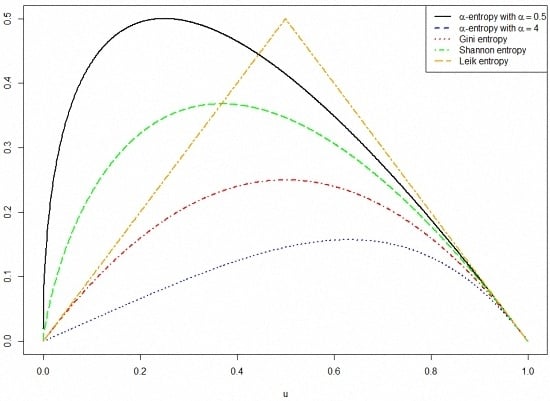
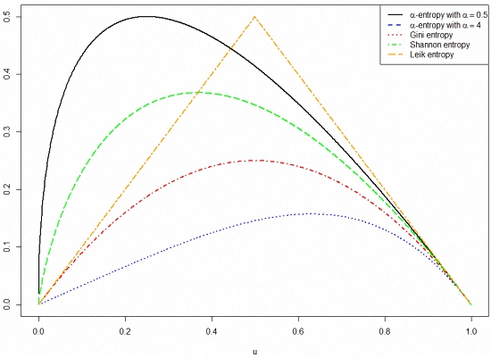
- Cumulative paired α-entropy : Following [57], let φ be given byfor . The corresponding so-called cumulative paired α-entropy is
- Cumulative paired Gini entropy : For we getas a special case of .
- Cumulative paired Shannon entropy : Set , . Thus,gives the entropy which was already mentioned in the introduction. It is a special case of for .
- Cumulative paired Leik entropy : The functionrepresents the limiting case of a linear concave function φ. The measure of dispersion proposed by [22] implicitly makes use of φ such that we callcumulative paired Leik entropy.
Figure 1 gives an impression of the previously mentioned generating functions φ .
3.2. Advantages of Entropies Based on Cdfs
The authos of [46,47] list several reasons for better defining an entropy for distribution functions rather than defining it for density functions. Starting point is the well-known critique of Shannon’s differential entropy that was expressed by several authors like [48,58] and (p. 58f) in [59].
Transferred to cumulative paired entropies, the advantages of entropies based on distribution functions (cf. [46]) are as follows:
- is based on probabilities and has a consistent definition for both discrete and continuous random variables.
- is always non-negative.
- can easily be estimated by the empirical distribution function. This estimation is strongly consistent, due to the strong consistency of the empirical distribution function.
Problems of the differential entropy are occasionally discussed in case of grouped data, at which the usual Shannon entropy is calculated for each group probability. With an increasing amount of groups, the Shannon entropy not only does not converge to the respective differential entropy, but it even diverges (cf., e.g., (p. 54) in ([59], (p. 239) in [60]). In the next section we will show that the discrete version of converges to as the number of groups approaches infinity.
3.3. for Grouped Data
First, we show the notation for characterizing grouped data. The interval is divided into k subintervals with limits . The range of each group is called for . Let X be a random variable with absolute continuous distribution function F, which is only known at the limits of each group. The probabilities of each group are denoted by , . is the random variable whose distribution function is yielded by linear interpolation of the values of F at the limits of successive groups. Finally, is the result of adding an independent, uniformly distributed random variable to X. It holds that
for , for and for .
Let denote the respective random variable of . The probability density function of is defined by for , .
Lemma 1.
Let φ be an entropy generating function with antiderivative . The paired cumulative φ-entropy of the distribution function in Equation (12) is given as follows:
Proof.
For , we have
with , , , and , . With and we have
☐
Considering this result, we can easily prove the convergence property for :
Theorem 1.
Let φ be a generating function with antiderivative and let F be a continuous distribution function of the random variable X with support . is the corresponding random variable for grouped data with , . Then the following holds:
Proof.
Consider equidistant classes with , . Subsequently, Equation (13) results in
With we have such that for F continuous we get . The antiderivative has the derivative φ almost everywhere such that with
An analogue argument holds for the second term of Equation (14). ☐
In addition to this theoretical result we get the following useful expressions for for grouped data and a specific choice of φ as Corollary 1 shows:
Corollary 1.
Let φ be s.t.
where . Then for
and for
Proof.
Using the antiderivatives
since , it holds that
for . The results follow immediately. ☐
3.4. Alternative Representations of
In case holds and φ is differentiable, one can provide several alternative representations of in addition to Eqaution (7). These alternative representations will be useful in the following to find conditions ensuring the existence of and to find some simple estimators.
Proposition 1.
Let φ be a non-negative and differentiable function on the domain with derivative and . In this case, for with quantile function , density function f, and quantile density function , for , the following holds:
Proof.
Apply probability integral transform and partial integration. ☐
Due to it holds that
This property supports the understanding of being a covariance for which the Cauchy–Schwarz inequality gives an upper bound:
Corollary 2.
Let φ be a non-negative and differentiable function on the domain with derivative and . Then if U is uniformly distributed on and :
Proof.
Let , then since ,
☐
Depending on the context, we switch between these alternative representations of .
4. Sufficient Conditions for the Existence of CPE
4.1. Deriving an Upper Bound for
The Cauchy–Schwarz inequality for Equations (18) and (19), respectively, provides an upper bound for if the variance exists and
holds. The existence of the upper bound simultaneously ensures the existence of .
Proposition 2.
Let φ be a non-negative and differentiable function on the domain with derivative and . If Equation (20) holds, then for with and quantile function , we have
Proof.
The statement follows from
☐
Next, we consider the upper bound for the cumulative paired α-entropy:
Corollary 3.
Let X be a random variable having a finite variance. Then
for , with
for .
Proof.
For and , , we have
is required for the existence of . For we have and , , such that
☐
In the framework of uncertainty theory, the upper bound for the paired cumulative Shannon entropy was derived by [51] (see also [6], p. 83). For we get the upper bound for the paired cumulative Gini entropy
This result has already been proven for non-negative uncertainty variables by [40]. Finally, one yields the following upper bound for the paired cumulative Leik entropy:
Corollary 4.
Let X be a random variable with existing variance. Then
Proof.
Use
to get the result. ☐
4.2. Stricter Conditions for the Existence of
So far, we only considered sufficient conditions for an existing variance. Following the arguments in [46,50], which were used for the special case of cumulative residual and residual Shannon entropy, one can derive stricter sufficient conditions for the existence of .
Theorem 2.
If for , then for .
Proof.
To prepare the proof we first note that
holds for and .
The second fact required for the proof is that
if , because
Third, it holds that
because
consists of four indefinite integrals:
It must be shown separately that these integrals converge.
The convergence of the first two terms follows directly from the existence of . With Equations (27) and (28) we have for
and
For the third term we have to demonstrate that
for . If , there is a β with while . With Equation (27) it is for that
because .
With there exists
For the transformation is monotonically increasing for . Using the Markov inequality we get
Putting these results together, we attain
for (and thus for ) and due to for .
It remains to show the convergence of the fourth term:
for . For , there is a β with and . Due to Equation (27) and for it is true that
With we have
Now, the Markov inequality gives
In summary, we have
for and by for . This completes the proof. ☐
Following Theorem 2, depending on the number of existing moments, specific conditions for α arise in order to ensure the existence of :
- If the variance of X exists (i.e., ), exists for .
- For , is sufficient for the existence of (i.e., ).
- For , is sufficient for the existence of (i.e., ).
5. Maximum CPE Distributions
5.1. Maximum Distributions for Given Mean and Variance
Equality in the Cauchy–Schwarz inequality gives a condition under which the upper bound is attained. This is the case if an affine linear relation between respectively X and respectively exists with probability 1. Since the quantile function is monotonically increasing, such an affine linear function can only exist if is monotonic as well (de- or increasing). This implies that φ needs to be a concave function on . In order to derive a maximum distribution under the restriction that mean and variance are given, one may only consider concave generating functions φ.
We summarize this obvious but important result in the following Theorem:
Theorem 3.
Let φ be a non-negative and differentiable function on the domain with derivative and . Then F is the maximum distribution with prespecified mean μ and variance of iff a constant exists such that
Proof.
The upper bound of the Cauchy–Schwarz inequality will be attained if there are constants such that the first restriction equals
The property leads to such that
This means that there is a constant with
The second restriction postulates that
φ is concave on with
Therefore, is monotonically increasing. The quantile function is also monotonically increasing such that b has to be positive. This gives
☐
The quantile function of the Tukey’s λ distribution is given by
Its mean and variance are
The domain is given by for .
By discussing the paired cumulative α-entropy, one can prove the new result that the Tukey’s λ distribution is the maximum distribution for prespecified mean and variance. Tukey’s λ distribution takes on the role of the Student-t distribution if one changes from the differential entropy to (cf. [61]).
Corollary 5.
The cdf F maximizes for under the restrictions of a given mean μ and given variance iff F is the cdf of the Tukey λ distribution with .
Proof.
For , , we have
for . As a consequence, the constant b is given by
and the maximum distribution results in
can easily be identified as the quantile function of a Tukey’s λ distribution with and . ☐
For the Gini case (), one obtains the quantile function of a uniform distribution
with domain . This maximum distribution corresponds essentially to the distribution derived by Dai et al. [40].
The fact that the logistic distribution is the maximum distribution, provided mean and variance are given, was derived by Chen et al. [51] in the framework of uncertainty theory and by ([50], p. 4) in the framework of reliability theory. Both proved this result using Euler–Lagrange equations. In the interest of completeness, we provide an alternative proof via the upper bound of the Cauchy–Schwarz inequality.
Corollary 6.
The cdf F maximizes under the restrictions of a known mean μ and a known variance iff F is the cdf of a logistic distribution.
Proof.
Since
one receives
Inverting gives the distribution function of the logistic distribution with mean μ and variance 1:
☐
As a last example we consider the cumulative paired Leik entropy .
Corollary 7.
The cdf F maximizes under restrictions of a known mean μ and a known variance iff for F holds
Proof.
From and , , follows that
☐
Therefore, the maximization of with given mean and variance leads to a distribution whose variance is maximal on the interval .
5.2. Maximum Distributions for General Moment Restrictions
Drissi et al. [50] discuss general moment restrictions of the form
for which the existence of the moments is assumed. By using Euler–Lagrange equations they show that
maximizes the residual cumulative entropy under constraints Equation (31). Moreover, they demonstrated that the solution needs to be symmetric with respect to μ. Here, , , are the Lagrange parameters which are determined by the moment restrictions, provided a solution exists. Rao et al. [47] shows that for distributions with support the ME distribution is given by
if the restrictions Equation (31) are again required.
One can easily examine the shape of a distribution which maximizes the cumulative paired φ-entropy under the constraints Equation (31). This maximum distribution can no longer be derived by the upper bound of the Cauchy–Schwarz inequality if . One has to solve the Euler–Lagrange equations for the objective function
with Lagrange parameters , . The Euler–Lagrange equations lead to the optimization problem
for . Once again there is a close relation between the derivative of the generating function and the quantile function, provided a solution of the optimization problem Equation (32) exists.
The following example shows that the optimization problem Equation (32) leads to a well-known distribution if constraints are chosen carefully in case of a Shannon-type entropy.
Example 1.
The power logistic distribution is defined by the distribution function
for . The corresponding quantile function is
This quantile function is also solution of Equation (33) given , , under the constraint . The maximum of the cumulative paired Shannon entropy under the constraint is given by
Setting leads to the familiar result for the upper bound of given the variance.
5.3. Generalized Principle of Maximum Entropy
Kesavan et al. [19] introduced the generalized principle of an ME problem which describes the interplay of entropy, constraints, and distributions. A variation of this principle is the aim of finding an entropy that is maximized by a given distribution and some moment restrictions.
This problem can easily be solved for if mean and variance are given, due to the linear relationship between and the quantile function of the maximum distribution provided by the Cauchy–Schwarz inequality. However, it is a precondition for that is strictly monotonic on in order to be a quantile function. Therefore, the concavity of and the condition are of key importance.
We demonstrate the solution to the generalized principle of the maximum entropy problem for the Gaussian and the Student-t distribution.
Proposition 3.
Let φ, Φ and be the density, the cdf and the quantile function of a standard Gaussian random variable. The Gaussian distribution is the maximum distribution for a given mean μ and variance for with entropy generating function
Proof.
With
the condition for the maximum distribution with mean μ and variance becomes
By substituting , it follows that
such that is the quantile function of a Gaussian distribution with mean μ and variance . ☐
An analogue result holds for the Student-t distribution with k degrees of freedom. In this case, the main difference to the Gaussian distribution is the fact that the entropy generating function possesses no closed form but is obtained by numerical integration of the quantile function.
Corollary 8.
Let respectively be the cdf respectively the quantile function of a Student-t distribution with k degrees of freedom for . is the maximum quantile function for a given mean μ and variance iff
Proof.
Starting with
and the symmetry of the distribution around μ, we get the condition
With we get the quantile function of the t distribution with k degrees of freedom and mean μ:
☐
Figure 2 shows the shape of the entropy generating function φ for several distributions generated by the generalized ME principle.
6. CPE as a Measure of Scale
6.1. Basic Properties of
The cumulative residual entropy () introduced by [46], the generalized cumulative residual entropy (GCRE) of [50], and the cumulative entropy () discussed by [8,9], have always been interpreted as measures of information. However, all these approaches do not explain which kind of information was considered. In contrast to this interpretation as measures of information, Oja [3] proved that the differential entropy satisfies a special ordering of scale and has certain meaningful properties of measures of scale. In [4], the authors discussed the close relationship between differential entropy and variance. In the discrete case the Shannon entropy can be interpreted as a measure of diversity, which is a concept of dispersion if there is no ordering and no distance between the realizations of a random variable. In this section, we will clarifying the important role which the variance plays for the existence of .
Therefore, we intend to provide a deeper insight in as a proper MOS. We start by showing that has typical properties of an MOS. In detail, a proper MOS should always be non-negative and attain its minimal value 0 for a degenerated distribution. If a finite interval is considered as support, an MOS should attain its maximum if a and b occur with probability . possesses all these properties as shown in the next proposition.
Proposition 4.
Let with for and . Let X be a random variable with support D and is assumed to exist. Then the following properties hold:
- 1.
- .
- 2.
- iff there exists an with .
- 3.
- attains its maximum iff there exist with such that .
Proof.
- Follows from the non-negativity of φ.
- If there is an with , then and for all . Due to follows for all .Set . Due to the non-negativity of the integrand of , must hold for . Since , , it follows , for .
- Let have a finite maximum. Since has a unique maximum at , the maximum of isIn order to attain the assumed finite maximum, the support D has to be a finite interval . Here, is the maximum. Now, it is sufficient to construct a distribution with support that attains this maximum. Setthen . Therefore, F is -maximal.To prove the other direction of statement 3 we consider an arbitrary distribution G with survival function and support . Due to and , it holds that☐
6.2. and Oja’s Axioms for Measures of Scale
Oja ([3] p. 159) defined a MOS as follows:
Definition 2.
Let be a set of continuous distribution functions and ⪯ an appropriate ordering of scale on . is called MOS, if
- 1.
- for all , .
- 2.
- , for , , with .
Oja [3] discussed several orderings of scale. He showed in particular that Shannon entropy and variance satisfy a partial quantile based ordering of scale, which has been discussed by [62]. Referring to [63,64] criticized that this ordering and the location-scale family of distributions focused by Oja [3] were too restrictive. He discussed a more general nonparametric model of dispersion based on a more general ordering of scale (cf. [65,66]). In line with [4], we focus on the scale ordering proposed by [62].
Definition 3.
Let , be continuous cdfs with respective quantile functions and . is said to be more spread out than () if
If , are absolutely continuous with density functions , , can be characterized equivalently by the property that is monotonically non-decreasing or
(cf. [3], p. 160).
Next, we show that is an MOS in the sense of [3]. This following lemma examines the behavior of with respect to affine linear transformations, referring to the first axiom of Definition 2:
Lemma 2.
Let F be the cdf of the random variable X. Then
Proof.
For , it follows that
Substitution of with gives
Likewise, we have that
such that
☐
In order to satisfy the second axiom of Oja’s definition of a measure of scale, has to satisfy the ordering of scale ⪯. This is shown by the following lemma:
Lemma 3.
Let and be continuous cdfs of the random variables and with . Then the following holds:
Proof.
One can show with that
for . Therefore,
If and hence for , it follows that . ☐
As a consequence of Lemma 2 and Lemma 3, is an MOS in the sense of [3]. Thus, not only variance, differential entropy, and other statistical measures have the properties of measures of scale, but also .
6.3. and Transformations
Ebrahimi et al. ([4] p. 323), the authors considered cdf , on domain , and density functions , , which are connected via , , via a differentiable transformation , that is respectively for . Thus, they demonstrated for Shannon’s differential entropy H that the transformation only affects the difference:
For , one gets a less explicit relationship between and :
Transformations with , , are of special interest since these transformations do not diminish measures of scale. In Theorem 1, Ebrahimi et al. [4] showed that holds if for . Hence, no MOS can be diminished by this specific transformation, especially neither Shannon entropy nor .
Ebrahimi et al. [4] considered the special transformation , . They showed that Shannon’s differential entropy is moved additively by this transformation, which is not expected for an MOS. Furthermore, the standard deviation is changed by the factor , which is also true for as shown in Lemma 2.
6.4. for Sums of Independent Random Variables
As is generally known, variance and differential entropy behave additively for the sum of independent random variables X and Y. More general entropies such as the Rényi or the Havrda & Charvát entropy are only subadditive (cf. [18], p. 194).
Neither the property of additivity nor the property of subadditivity could be shown for cumulative paired φ-entropies. Instead, they possess the maximum property if φ is a concave function on . This means that, for two independent variables X and Y, is lower-bounded by the maximum of the two individual entropies and . This result was shown by [46] for the cumulative residual Shannon entropy. The following Theorem generalizes this result, while the proof partially follows Theorem 2 of [46].
Theorem 4.
Let X and Y be independent random variables and φ a concave function on the interval with . Then we have
Proof.
Let X and Y be independent random variables with distribution functions , and densities , . Using the convolution formula, we immediately get
The existence of the expectation is assumed. To prove the Theorem, we begin with
In the context of uncertainty theory, Liu [6] considered a different definition of independence for uncertain variables leading to the simpler additivity property
for independent uncertain variables X and Y.
7. Estimation of CPE
Beirlant et al. [67] presented an overview of differential entropy estimators. Essentially, all proposals are based on the estimation of a density function f inheriting all typical problems of nonparametric estimation of a density function. Among others, the problems are biasedness, choice of a kernel, and optimal choice of the smoothing parameter (cf. [68], p. 215ff.). However, is based on cdf F for which several natural estimators with desirable stochastic properties, derived from the Theorem of Glivenko and Cantelli (cf. [69], p. 61), exist. For a simple random sample , independently distributed random variables with identical distribution function F, the authors of [8,9] estimated F using the empirical distribution function for . Moreover, they showed for the cumulative entropy that the estimator is consistent for (cf. [8]). In particular, for F being the distribution function of a uniform distribution, they provided the expected value of the estimator and demonstrated that the estimator is asymptotically normal. For F being the cdf of an exponential distribution, they additionally derived the variance of the estimator.
In the following, we generalize the estimation approach of [8] by embedding it into the well-established theory of L-estimators (cf. [70], p. 55ff.). If φ is differentiable, then can be represented as the covariance between the random variable X and :
An unbiased estimator for this covariance is
where
This results in an L-estimator with , . By applying known results for the influence functions of L-estimators (cf. [70]), we get for the influence function of :
In particular, the derivative is
This means that the influence function will be completely determined by the antiderivative of . The following examples demonstrate that the influence function of can easily be calculated if the underlying distribution F is logistic. We consider the Shannon, the Gini, and the α-entropy cases.
Example 2.
Beginning with the derivative
we arrive at
The influence function is not bounded and proportional to the influence function of the variance, which implies that variance and have a similar asymptotic and robustness behavior. The integration constant C has to be determined such that
Example 3.
Using the Gini entropy and the logistic distribution function F we have
Integration gives the influence function
By applying numerical integration we get .
Example 4.
For the derivative of the influence function is given by
Integration leads to the influence function
where
Under certain conditions (cf. [71], p. 143) concerning J, or φ and F, L- estimators are consistent and asymptotically normal. So, the cumulative paired φ-entropy is
with asymptotic variance
The following examples consider the Shannon and the Gini case for which the condition that is sufficient to guarantee asymptotic normality can easily be checked. We consider again the cdf F of the logistic distribution.
Example 5.
For the cumulative paired Shannon entropy it holds that
since
Example 6.
In the Gini case we get
since by numerical integration
It is known that L-estimators have a remarkable small-sample bias. Following [72], the bias can be reduced by applying the Jackknife method. It is well-known that asymptotical distributions can be used to construct approximate confidence intervals as well as that they can be applied for hypothesis tests in the one- or two-sample case. ([70], p. 116ff.) discussed asymptotic efficient L-estimators for a parameter of scale θ. Klein et al. [73] examine how the entropy generating function φ will be determined by the requirement that has to be asymptotically efficient.
8. Related Concepts
Several statistical concepts are closely related to cumulative paired φ-entropies. These concepts generalize some results which are known from literature. We begin with the cumulative paired φ-divergence that was discussed for the first time by [41], who called it “generalized cross entropy”. Their focus was on uncertain variables, whereas ours is on random variables. The second concept generalizes mutual information, which is defined for Shannon’s differential entropy, to mutual φ-information. We consider two random variables X and Y. The task is to decompose into two kinds of variation such that the so-called external variation measures how much of can be explained by X. This procedure mimics the well-known decomposition of variance and allows to define directed measures of dependence for X and Y. The third concept deals with dependence. More precisely, we introduce a new family of correlation coefficients that measure the strength of a monotonic relationship between X and Y. Well-known coefficients like the Gini correlation can be embedded in this approach. The fourth concept treats the problem of linear regression. can serve as general measure of dispersion that has to be minimized to estimate the regression coefficients. This approach will be identified as a special case of rank-based regression or R regression. Here, the robustness properties of the rank-based estimator can directly be derived from the entropy generating function φ . Moreover, asymptotics can be derived from theory of rank-based regression. The last concept we discuss applies to linear rank tests for the difference of scale. Known results, especially concerning the asymptotics, can be transferred from the theory of linear rank tests to this new class of tests. In this paper, we only sketch the main results and focus on examples. For a detailed discussion including proofs we refer to a series of papers by Klein and Mangold ([73,74,75]) , which are currently work in progress.
8.1. Cumulative Paired φ-Divergence
Let φ be a concave function defined on with . Additionally, we need . In the literature, φ-divergences are defined for convex functions φ (cf., e.g., [76], p. 5). Consequently, we consider with φ concave.
The cumulative paired φ-divergence for two random variables is defined as follows.
Definition 4.
Let X and Y be two random variables with cdfs and . Then the cumulative paired φ-divergence of X and Y is given by
The following examples introduce cumulative paired φ-divergences for the Shannon, the α-entropy, the Gini, and the Leik cases:
Example 7.
- 1.
- Considering , , we obtain the cumulative paired Shannon divergence
- 2.
- Setting , , leads to the cumulative paired α-divergence
- 3.
- For we receive as a special case the cumulative paired Gini divergence
- 4.
- The choice , , leads to the cumulative paired Leik divergence
is equivalent to the Anderson-Darling functional (cf. [77]) and has been used by [78] for a goodness-of-fit test, where represents the empirical distribution. Likewise, serves as a goodness-of-fit test (cf. [79]).
Further work in this area with similar concepts was done by [80,81], using the notation cumulative residual Kullback-Leiber (CRKL) information and cumulative Kullback-Leiber (CKL) information.
Up to a multiplicative constant, includes all of the aforementioned examples. In addition, the Hellinger distance is a special case for that leads to the cumulative paired Hellinger divergence:
For a strictly concave function φ, Chen et al. [41] proved that and iff X and Y have identical distributions. Thus, the cumulative paired φ-divergence can be interpreted as a kind of a distance between distribution functions. As an application, Chen et al. [41] mentioned the “minimum cross-entropy principle”. They proved that X follows a logistic distribution if is minimized, given that Y is exponentially distributed and the variance of X is fixed. If is an empirical distribution and has an unknown vector of parameters θ, can be minimized to attain a point estimator for θ (cf. [87]). The large class of goodness-of-fit tests based on , discussed by Jager et al. [86], has already been mentioned.
8.2. Mutual Cumulative φ-Information
Let X and Y again be random variables with cdfs , , density functions , , and the conditional distribution function . and denote the supports of X and Y. Then we have
which is the variation of Y given . Averaging with respect to x leads to the internal variation
For a concave entropy generating function φ, this internal variation cannot be greater than the total variation . More precisely, it holds:
- .
- if X and Y are independent.
- If φ is strictly concave and , X and Y are independent random variables.
We consider the non-negative difference
This expression measures the part of the variation of Y that can be explained by the variable X (= external variation) and shall be named “mutual cumulative paired φ-information” (cf. Rao et al. [46] using the term “cross entropy”, (p. 3) in [50]). is equivalent to the transinformation that is defined for Shannon’s differential entropy (cf. [60], p. 20f.). In contrast to transinformation, is not symmetric, so is not true in general.
Cumulative paired mutual φ-information is the starting point for two directed measures of strength of φ-dependence between X and Y, namely “directed (measure) of cumulative paired φ-dependence”, . The first one is
and the second one is
Both expressions measure the relative decrease in variation of Y if X is known. The domain is . The lower bound 0 is taken if Y and X are independent, while the upper bound 1 corresponds to . In this case, from for and , we can conclude that the conditional distribution has to be degenerated. Thus, for every there is exactly one with . Therefore, there is a perfect association between X and Y. The next example illustrates these concepts and demonstrates the advantage of considering both types of measures of dependence.
Example 8.
Let follow a bivariate standard Gaussian distribution with , , and , . Note that X and Y follow univariate standard Gaussian distributions, whereas follows a univariate Gaussian distribution with mean 0 and variance . Considering this, one can conclude that
By plugging this quantile function into the defining equation of the cumulative paired φ-entropy one yields
For , the cumulative paired φ-entropy behaves like the variance or the standard deviation. All measures approach 0 for , such that can be used as a measure of risk since the risk can be completely eliminated in a portfolio with perfectly negative correlated returns of assets. To be more precise, it is to say that rather behaves like the standard deviation than the variance.
For , the variance of the sum equals the sum of the variances, but the standard deviation of the sum is equal to or smaller than the sum of the individual standard deviations. This is also true for .
In case of the bivariate standard Gaussian distribution, is Gaussian as well with mean and variance for and . Therefore, the quantile function of is
Using this quantile function, the cumulative paired φ-entropy for the conditional random variable is
Just like the variance of , does not depend on x in case of a bivariate Gaussian distribution. This implies that the internal variation is , as well.
For , the bivariate distribution becomes degenerated and the internal variation consequently approaches 0. The mutual cumulative paired φ-information is given by
takes the value 0 if and only if , in which case X and Y are independent.
The two measures of directed cumulative φ-dependence for this example are
and
ρ completely determines the values for both measures of directed dependence. Provided the upper bound 1 will be attained, there is a perfect linear relation between Y and X.
As a second example we consider the dependence structure of the Farlie-Gumbel-Morgenstern copula (FGM copula). For the sake of brevity, we define a copula C as bivariate distribution function with uniform marginals for two random variables U and V with support . For details concerning copulas see, e.g., [88].
Example 9.
Let
be the FGM copula (cf. [88], p. 68). With
it holds for the conditional cumulative φ-entropy of U given that
To get expressions in closed form we consider the Gini case with , . After some simple calculations we have
Averaging over the uniform distribution of V leads to the internal variation
With , the mutual cumulative Gini information and the directed cumulative measure of Gini dependence are
It is well-known that only a small range of dependence can be covered by the FGM copula (cf. [88], p. 129).
Hall et al. [89] discussed several methods for estimating a conditional distribution. The results can be used for estimating the mutual φ-information and the two directed measures of dependence. This will be the task of future research.
8.3. φ-Correlation
Schechtman et al. [90] introduced Gini correlations of two random variables X and Y with distribution functions and as
The numerator equals of the Gini mean difference
where the expectation is calculated for two independent and with identically distributed random variables and .
Gini’s mean difference coincides with the cumulative paired Gini entropy in the following way:
Therefore, in the same way that Gini’s mean difference can be generalized to the Gini correlation, can be generalized to the φ-correlation.
Let be two random variables and let , be the corresponding cumulative paired φ-entropies, then
and
are called φ-correlations of X and Y. Since , the numerator is the covariance between X and .
The first example verifies that the Gini correlation is a proper special case of the φ-correlation.
Example 10.
The setting , , leads to the Gini correlation, because
and
The second example considers the new Shannon correlation.
Example 11.
Set , , then we get the Shannon correlation
If Y follows a logistic distribution with , , then . Considering this, we get
From Equation (30) we know that if X is logistically distributed. In this specific case we get
In the following example we introduce the α-correlation.
Example 12.
For , , we get the α-correlation
For , , we get
The authors of [90,91,92] proved that Gini correlations possess many desirable properties. In the following we give an overview of all properties which can be transferred to φ-correlations. For proofs and further details we refer to [75].
We start with the fact that φ-correlations also have a copula representation since for the covariance holds
The following examples demonstrate the copula representation for the Gini and the Shannon correlation.
Example 13.
In the Gini case it is . This leads to
Example 14.
In the Shannon case, such that
The following basic properties of φ-correlations can easily be checked with the arguments applied by [90]:
- .
- if there is a strictly increasing (decreasing) transformation g such that .
- If g is monotonic, then .
- If g is affin-linear, then .
- If X and Y are independent, then .
- If and are exchangeable for some constants with , then .
In the last subsection we have seen that two directed measures of φ-dependence do not rely on φ if a bivariate Gaussian distribution is considered. The same holds for φ-correlations as will be demonstrated in the following example.
Example 15.
Let be a bivariate standard Gaussian random variable with Pearson correlation coefficient ρ. Thus, all φ-correlations coincide with ρ as the following consideration shows:
With it is
Dividing this by yields the result.
Weighted sums of random variables appear for example in portfolio optimization. The diversification effect concerns negative correlations between the returns of assets. Thus, the risk of a portfolio can be significantly smaller than the sum of the individual risks. Now, we analyze whether cumulative paired φ-entropies can serve as a risk measure as well. Therefore, we have to examine the diversification effect for .
First, we display the total risk as a weighted sum of individual risks. Essentially, the weights need to be the φ-correlations of the individual returns with the portfolio return: Let , then it holds that
For the diversification effect the total risk has to be displayed as a function of the φ-correlations between and , . A similar result was provided by [92] for the Gini correlation without proof. Let and set , , then the following decomposition of the square of holds:
This is similar to the representation for the variance of Y, where takes the role of the Pearson correlation and the role of the standard deviation for .
Schechtman et al. [90] also introduced an estimator for the Gini correlation and derived its asymptotic distribution. For the proof it is useful to note that the numerator of the Gini correlation can be represented as a U-statistic. For the general case of the φ-correlation it is necessary to derive the influence function and to calculate its variance. This will be done in [75].
8.4. φ-Regression
Based on the Gini correlation Olkin et al. [93] considered the traditional ordinary least squares (OLS) approach in regression analysis
where Y is the dependent variable and x is the independent variable. They modified it by minimizing the covariance between the error term ε in a linear regression model and the ranks of ε with respect to α and β. Ranks are the sample analogue of the theoretical distribution function , such that the Gini mean difference is the center of this new approach for regression analysis. Olkin et al. [93] noticed that this approach is already known as “rank based regression” or short “R regression” in robust statistics. In robust regression analysis the more general optimization criteria has been considered, where φ denotes a strictly increasing score function (cf. [94], p. 233). The choice leads to the Gini mean difference, which is the scores generating function of the Wilcoxon scores. The rank based regression approach with general scores generating function , , is equivalent to the generalization of the Gini regression to a so-called φ-regression based on the criteria function
which has to be minimized to obtain α and β. Therefore, cumulative paired φ-entropies are special cases of the dispersion function that [95,96] proposed as optimization criteria for R regression. More precisely, R estimation proceeds in two steps. In the first step
has to be minimized with respect to β. Let denote this estimator. In the second step α will be estimated separately by
The authors of [97,98] gave an overview of recent developments in rank based regression. We will apply their main results to φ-regression. In [99], the authors showed that the following property holds for the influence function of :
where represents an outlier. determines the influence of an outlier in the dependent variable on the estimator .
The scale parameter is given by
The influence function shows that is asymptotically normal:
For bounded, Koul et al. [100] proposed a consistent estimator for the scale parameter . This asymptotic property can again be used to construct approximate confidence limits for the regression coefficients, to derive a Wald test for the general linear hypothesis, to derive a goodness-of-fit test, and to define a measure of determination (cf. [97])).
Gini regression corresponds to . In the same way we can derive from the new Shannon regression, from the α-regression, and from the Leik regression.
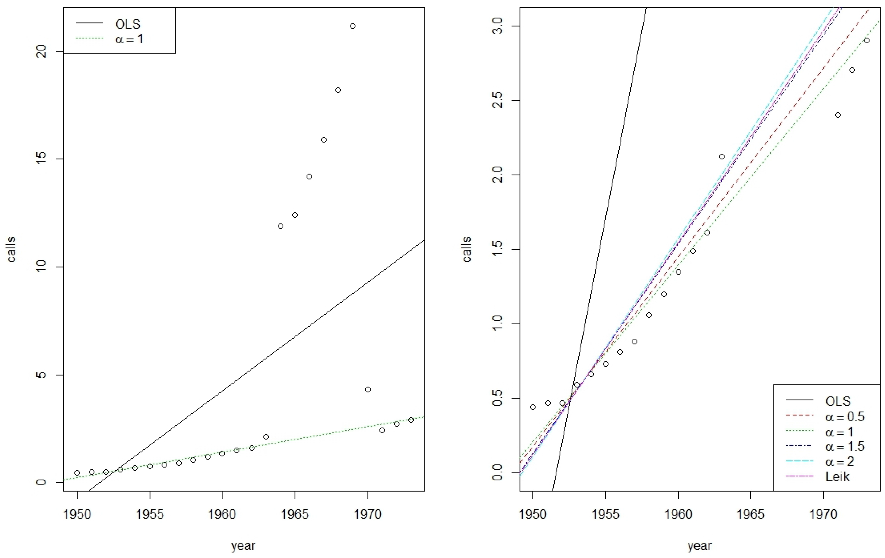
The R package “Rfit” has the option to include individual φ-functions into rank based regression (cf. [97]). Using this option and the dataset “telephone”, which is available with several outliers in “Rfit”, we compare the fit of the Shannon regression ), the Leik regression, and the α-regression (for several values of α) with the OLS regression. Figure 3 shows on the left the original data, the OLS, and the Shannon regression, while on its right side outliers were excluded to get a more detailed impression of the differences between the φ-regressions.
In comparison with the very sensitive OLS regression all rank based regression techniques behave similarly. In case of a known error distribution, McKean et al. [98] showed an asymptotically efficient estimator for . This procedure also determines the entropy generating function φ. In case of an unknown error distribution but some available information with respect to skewness and leptokurtosis, a data-driven (adaptive) procedure was proposed by them.
8.5. Two-Sample Rank Test on Dispersion
Based on the linear rank statistics
can be used as a test statistic for alternatives of scale, where are the ranks of in the pooled sample . All random variables are assumed to be independent.
Some of the linear rank statistics which are well-known from the literature are special cases of Equation (56) as will be shown in the following examples:
Example 16.
Let , , then we have
Ansari et al. [101] suggest the statistic
as a two-sample test for alternatives of scale (cf. [102], p. 104). Apparently, we have .
Example 17.
In the following, the scores of the Mood test will be generated by the generating function of .
Dropping the requirement of concavity of φ, one finds analogies to other well-known test statistics.
Example 18.
Let , , which is not concave on the interval [0,1], we have
which is identical to the quantile test statistic for alternatives of scale up to an affine linear relation ([102], p. 105).
The asymptotic distribution of linear rank tests based on can be derived from the theory of linear rank test, as discussed in [102]. The asymptotic distribution under the null hypothesis is needed to be able to make an approximate test decision given a significance level α. The asymptotic distribution under the alternative hypothesis is needed for an approximate evaluation of the test power and the choice of the required sample size in order to ensure a given effect size, respectively.
We consider the centered linear rank statistic
Under the null hypothesis of identical scale parameters and the assumption that
where , the asymptotical distribution of is given by
(cf. [102], p. 194, Theorem 1 and p. 195, Lemma 1).
The property of asymptotic normality of the Ansari-Bradley test and the Mood test is well-known. Therefore, we provide a new linear rank test based on cumulative paired Shannon entropy (so-called “Shannon”-test) in the following example:
Example 19.
With , , and we have
and
Under the null hypothesis of identical scale, the centered linear rank statistic is asymptotically normal with variance
If the alternative hypothesis for a density function is given by
for and , then set
and assume . If and with , is asymptotically normal distributed with mean
and variance
This result follows immediately from [102], p. 267, Theorem 1, together with the Remark on, p. 268.
If is a symmetric distribution, , , holds such that
This simplifies the variance of the asymptotic normal distribution.
Since the asymptotic normality of the test statistic of the Ansari-Bradley test and the Mood test under the alternative hypothesis have been examined intensely (cf., e.g., [103,104]), we focus in the following example on the new Shannon test:
Example 20.
Set , and let be the density function of a standard Gaussian distribution, such that and . As a consequence, we have
and
where the integrals have been evaluated by numerical integration. Then under the alternative Equation (58):
Hereafter, one can discuss the asymptotic efficiency of linear rank tests based on cumulative paired φ-entropy. If is the true density and
then gives the desired asymptotic efficiency (cf. [102], p. 317).
The asymptotic efficiency of the Ansari-Bradley test (and the asymptotic equivalent Siegel-Tukey test, respectively) and the Mood test have been analyzed by [104,105,106]. The asymptotic relative efficiency (ARE) with respect to the traditional F-test for differences in scale for two Gaussian distributions has been discussed by [103]. This asymptotic relative efficiency between Mood test and F-test for differences in scale has been derived by [107]. Once more, we focus on the new Shannon-test.
Example 21.
The Klotz test is asymptotically efficient for the Gaussian distribution. With ,
gives the asymptotic efficiency of the new Shannon test.
Using a distribution that ensures the asymptotic efficiency of the Ansari-Bradley test, we compare the asymptotic efficiency of the Shannon test to the one of the Ansari-Bradley test.
Example 22.
The Ansari-Bradley test statistic is asymptotically efficient for the double log-logistic distribution with density function (cf. [102], p. 104). The Fisher information is given by
Furthermore, we have
such that the asymptotic efficiency of the Shannon-test for is
These two examples show that the Shannon test has a rather good asymptotic efficiency, even if the underlying distribution has moderate tails similar to the Gaussian distribution or heavy tails like the double log-logistic distribution. Asymptotic efficient linear rank tests correspond to a distribution and a scores generating function , from which we can derive an entropy generating function φ and a cumulative paired φ-entropy. This relationship will be further examined in [74].
9. Some Cumulative Paired Entropies for Selected Distribution Functions
In the following, we derive closed form expressions for some cumulative paired φ-entropies. We mimic the procedure of ([4], p. 326) to some degree. Table 1 of their paper contains multiple formulas of the differential entropy for the most popular statistical distributions. Several of these distributions will also be considered in the following. Since cumulative entropies depend on the distribution function or equivalently on the quantile function, we focus on families of distributions for which these functions have a closed form expression. Furthermore, we only discuss standardized random variables since the parameter of scale only has a multiplicative effect on and the parameter of location has no effect. For the standard Gaussian distribution we provide the value of by numerical integration rounded to two decimal places since the probability function has no explicit form. For the Gumbel distribution however, there is a closed form expression for the distribution function – nevertheless, we were unable to establish a closed form of and . Therefore, we applied numerical integration in this case as well. In the following, next to the Gamma function and the Beta function , we use
- the incomplete Gamma function
- the incomplete Beta function
- and the Digamma function
9.1. Uniform Distribution
Let X have the standard uniform distribution. Then we have
9.2. Power Distribution
Let X have the Beta distribution on with parameter and , i.e., density function for , then we have
9.3. Triangular Distribution with Parameter c
Let X have a triangular distribution with density function
Then the following holds:
9.4. Laplace Distribution
Let X follow the Laplace distribution with density function for , then we have
9.5. Logistic Distribution
Let X follow the logistic distribution with distribution function for , then we have
9.6. Tukey λ Distribution
Let X follow the Tukey λ distribution with quantile function for and . Then the following holds:
9.7. Weibull Distribution
Let X follow the Weibull distribution with distribution function for , , then we have
9.8. Pareto Distribution
Let X follow the Pareto distribution with distribution function for , , then we have
9.9. Gaussian Distribution
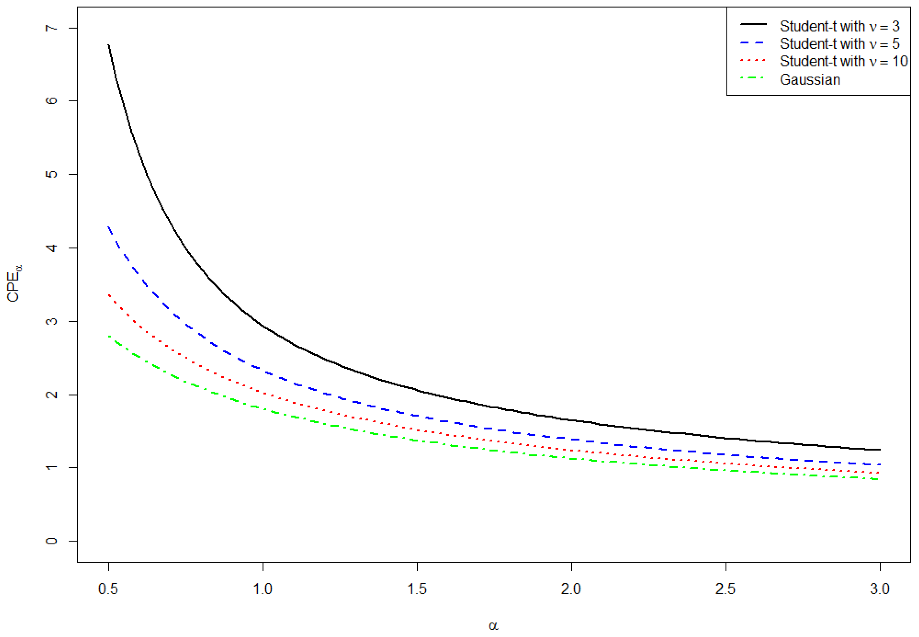
By means of numerical integration we calculated the following values for the standard Gaussian distribution:
for and the standard Gaussian distribution can be seen in Figure 4.
9.10. Student-t Distribution
By means of numerical integration and for degrees of freedom we calculated the following values for the Student-t distribution
As can be seen in Figure 4, the heavy tails of the Student-t distribution result in a higher value for as compared with the Gaussian distribution.
10. Conclusions
A new kind of entropy has been introduced that generalizes Shannon’s differential entropy. The main difference to the previous discussion of entropies is the fact that the new entropy is defined for distribution functions instead of density functions. This paper shows that this definition has a long tradition in several scientific disciplines like fuzzy set theory, reliability theory, and more recently in uncertainty theory. With only one exception within all the disciplines, the concepts had been discussed independently. Along with that, the theory of dispersion measures for ordered categorical variables refers to measures based on distribution functions, without realizing that implicitly some sort of entropies are applied. Using the Cauchy–Schwarz inequality, we were able to show the close relationship between the new kind of entropy named cumulative paired φ-entropy and the standard deviation. More precisely, the standard deviation yields an upper limit for the new entropy. Additionally, the Cauchy–Schwarz inequality can be used to derive maximum entropy distributions provided that there are constraints specifying values of mean and variance. Here, the logistic distribution takes on the same key role for the cumulative paired Shannon entropy which the Gaussian distribution takes by maximizing the differential entropy. As a new result we have demonstrated that Tukey’s λ distribution is a maximum entropy distribution if using the entropy generating function φ which is known from the Harvda and Charvát entropy. Moreover, some new distributions can be derived by considering more general constraints. A change in perspective allows to determine the entropy that will be maximized by a certain distribution if, e.g., mean and variance are known. In this context the Gaussian distribution gives a simple solution. Since cumulative paired φ-entropy and variance are closely related, we have investigated whether the cumulative paired φ-entropy is a proper measure of scale. We show that it satisfies the axioms which were introduced by Oja for measures of scale. Several further properties, concerning the behavior under transformations or the sum of independent random variables, have been proven. Consequently, we have given first insights on how to estimate the new entropy. In addition, based on cumulative paired φ-entropy we have introduced new concepts like φ-divergence, mutual φ-information, and φ-correlation. φ-regression and linear rank tests for scale alternatives were considered as well. Furthermore, formulas have been derived for some popular distributions with cdf or quantile function in closed form and for certain cumulative paired φ-entropies.
Acknowledgments
The authors would like to thank the anonymous reviewers for their constructive criticism, which helped to improve the presentation of this paper significantly. Furthermore, we would like to thank Michael Grottke for helpful advises.
Author Contributions
Ingo Klein conceived the new entropy concept, investigated its properties and wrote an initial version of the manuscript. Benedikt Mangold cooperated especially by checking, correcting and improving the mathematical details including the proofs. He examined the entropy’s properties by simulation. Monika Doll contributed by mathematical and linguistic revision. All authors have read and approved the final manuscript.
Conflicts of Interest
The authors declare no conflict of interest.
References
- Burbea, J.; Rao, C.R. On the convexity of some divergence measures based on entropy functions. IEEE Trans. Inf. Theory 1982, 28, 489–495. [Google Scholar] [CrossRef]
- Shannon, C.E. A mathematical theory of communication. Bell Syst. Tech. J. 1948, 27, 379–423. [Google Scholar] [CrossRef]
- Oja, H. On location, scale, skewness and kurtosis of univariate distributions. Scand. J. Stat. 1981, 8, 154–168. [Google Scholar]
- Ebrahimi, N.; Massoumi, E.; Soofi, E.S. Ordering univariate distributions by entropy and variance. J. Econometr. 1999, 90, 317–336. [Google Scholar] [CrossRef]
- Popoviciu, T. Sur les équations algébraique ayant toutes leurs racines réelles. Mathematica 1935, 9, 129–145. (In French) [Google Scholar]
- Liu, B. Uncertainty Theory. Available online: http://orsc.edu.cn/liu/ut.pdf (accessed on 27 June 2016).
- Wang, F.; Vemuri, B.C.; Rao, M.; Chen, Y. A New & Robust Information Theoretic Measure and Its Application to Image Alignment: Information Processing in Medical Imaging; Lecture Notes in Computer Science; Springer: Berlin/Heidelberg, Germany, 2003; Volume 2732, pp. 388–400. [Google Scholar]
- Di Crescenzo, A.; Longobardi, M. On cumulative entropies and lifetime estimation. In Methods and Models in Artificial and Natural Computation; Mira, J.M., Ed.; Springer: Berlin/Heidelberg, Germany, 2009; pp. 132–141. [Google Scholar]
- Di Crescenzo, A.; Longobardi, M. On cumulative entropies. J. Stat. Plan. Inference 2009, 139, 4072–4087. [Google Scholar] [CrossRef]
- Kapur, J.N. Derivation of logistic law of population growth from maximum entropy principle. Natl. Acad. Sci. Lett. 1983, 6, 429–433. [Google Scholar]
- Hartley, R. Transmission of information. Bell Syst. Tech. J. 1928, 7, 535–563. [Google Scholar] [CrossRef]
- De Luca, A.; Termini, S. A definition of a nonprobabilistic entropy in the setting of fuzzy set theory. Inf. Control 1972, 29, 301–312. [Google Scholar] [CrossRef]
- Zadeh, L. Probability measures of fuzzy events. J. Math. Anal. Appl. 1968, 23, 421–427. [Google Scholar] [CrossRef]
- Pal, N.R.; Bezdek, J.C. Measuring fuzzy uncertainty. IEEE Trans. Fuzzy Syst. 1994, 2, 107–118. [Google Scholar] [CrossRef]
- Rényi, A. On measures of entropy and information. In Fourth Berkeley Symposium on Mathematical Statistics and Probability; University of California Press: Oakland, CA, USA, 1961; pp. 547–561. [Google Scholar]
- Esteban, M.D.; Morales, D. A summary on entropy statistics. Kybernetika 1995, 31, 337–346. [Google Scholar]
- Cichocki, A.; Amari, S. Families of alpha- beta- and gamma-divergences: Flexible and robust measures of similarities. Entropy 2010, 12, 1532–1568. [Google Scholar] [CrossRef]
- Arndt, C. Information Measures; Springer: Berlin/Heidelberg, Germany, 2004. [Google Scholar]
- Kesavan, H.K.; Kapur, J.N. The generalizedmaximumentropy principle. IEEE Trans. Syst. Man Cyber. 1989, 19, 1042–1052. [Google Scholar] [CrossRef]
- Jaynes, E.T. Information theory and statistical mechanics. Phys. Rev. 1957, 106, 620–630. [Google Scholar] [CrossRef]
- Jaynes, E.T. Information theory and statistical mechanics. II. Phys. Rev. 1957, 108, 171–190. [Google Scholar] [CrossRef]
- Leik, R.K. A measure of ordinal consensus. Pac. Sociol. Rev. 1966, 9, 85–90. [Google Scholar] [CrossRef]
- Vogel, H.; Dobbener, R. Ein Streuungsmaß für komparative Merkmale. Jahrbücher für Nationalökonomie und Statistik 1982, 197, 145–157. (In German) [Google Scholar]
- Kvålseth, T.O. Nominal versus ordinal variation. Percept. Mot. Skills 1989, 69. [Google Scholar] [CrossRef]
- Berry, K.J.; Mielke, P.W. Assessment of variation in ordinal data. Percept. Motor Skills 1992, 74, 63–66. [Google Scholar] [CrossRef]
- Berry, K.J.; Mielke, P.W. Indices of ordinal variation. Percept. Motor Skills 1992, 74, 576–578. [Google Scholar] [CrossRef]
- Berry, K.J.; Mielke, P.W. A test of significance for the index of ordinal variation. Percept. Motor Skills 1994, 79, 291–1295. [Google Scholar]
- Blair, J.; Lacy, M.G. Measures of variation for ordinal data. Percept. Motor Skills 1996, 82, 411–418. [Google Scholar] [CrossRef]
- Blair, J.; Lacy, M.G. Statistics of ordinal variation. Sociol. Methods Res. 2000, 28, 251–280. [Google Scholar] [CrossRef]
- Gadrich, T.; Bashkansky, E.; Zitikas, R. Assessing variation: A unifying approach for all scales of measurement. Qual. Quant. 2015, 49, 1145–1167. [Google Scholar] [CrossRef]
- Allison, R.A.; Foster, J.E. Measuring health inequality using qualitative data. J. Health Econ. 2004, 23, 505–524. [Google Scholar] [CrossRef] [PubMed]
- Zheng, B. Measuring inequality with ordinal data: A note. Res. Econ. Inequal. 2008, 16, 177–188. [Google Scholar]
- Abul Naga, R.H.; Yalcin, T. Inequality measurement for ordered response health data. J. Health Econ. 2008, 27, 1614–1625. [Google Scholar] [CrossRef] [PubMed]
- Zheng, B. A new approach to measure socioeconomic inequality in health. J. Econ. Inequal. 2011, 9, 555–577. [Google Scholar] [CrossRef]
- Apouey, B.; Silber, J. Inequality and bi-polarization in socioeconomic status and health: Ordinal approaches. Res. Econ. Inequal. 2013, 21, 77–109. [Google Scholar]
- Klein, I. Rangordnungsstatistiken als Verteilungsmaßzahlen für ordinalskalierte Merkmale: I. Streuungsmessung. In Diskussionspapiere des Lehrstuhls für Statistik und; Ökonometrie der Universität: Erlangen-Nürnberg, Germany, 1999; Volume 27. (In German) [Google Scholar]
- Yager, R.R. Dissonance—A measure of variability for ordinal random variables. Int. J. Uncertain. Fuzzin. Knowl. Based Syst. 2001, 9, 39–53. [Google Scholar]
- Bowden, R.J. Information, measure shifts and distribution metrics. Statistics 2012, 46, 249–262. [Google Scholar] [CrossRef]
- Dai, W. Maximum entropy principle for quadratic entropy of uncertain variables. Available online: http://orsc.edu.cn/online/100314.pdf (accessed on 27 June 2016).
- Dai, W.; Chen, X. Entropy of function of uncertain variables. Math. Comput. Model. 2012, 55, 754–760. [Google Scholar] [CrossRef]
- Chen, X.; Kar, S.; Ralescu, D.A. Cross-entropy measure of uncertain variables. Inf. Sci. 2012, 201, 53–60. [Google Scholar] [CrossRef]
- Yao, K.; Gao, J.; Dai, W. Sine entropy for uncertain variables. Int. J. Uncertain. Fuzzin. Knowl. Based Syst. 2013, 21, 743–753. [Google Scholar] [CrossRef]
- Yao, K.; Ke, H. Entropy operator for membership function of uncertain set. Appl. Math. Comput. 2014, 242, 898–906. [Google Scholar] [CrossRef]
- Ning, Y.; Ke, H.; Fu, Z. Triangular entropy of uncertain variables with application to portfolio selection. Soft Comput. 2015, 19, 2203–2209. [Google Scholar] [CrossRef]
- Ebrahimi, N. How to measure uncertainty in the residual lifetime distribution. Sankhya Ser. A 1996, 58, 48–56. [Google Scholar]
- Rao, M.; Chen, Y.; Vemuri, B.C.; Wang, F. Cumulative residual entropy: A new measure of information. IEEE Trans. Inf. Theory 2004, 50, 1220–1228. [Google Scholar] [CrossRef]
- Rao, M. More on a new concept of entropy and information. J. Theor. Probabil. 2005, 18, 967–981. [Google Scholar] [CrossRef]
- Schroeder, M.J. An alternative to entropy in the measurement of information. Entropy 2004, 6, 388–412. [Google Scholar] [CrossRef]
- Zografos, K.; Nadarajah, S. Survival exponential entropies. IEEE Trans. Inf. Theory 2005, 51, 1239–1246. [Google Scholar] [CrossRef]
- Drissi, N.; Chonavel, T.; Boucher, J.M. Generalized cumulative residual entropy distributions with unrestricted supports. Res. Lett. Signal Process. 2008, 2008. [Google Scholar] [CrossRef]
- Chen, X.; Dai, W. Maximum entropy principle for uncertain variables. Int. J. Fuzzy Syst. 2011, 13, 232–236. [Google Scholar]
- Sunoj, S.M.; Sankaran, P.G. Quantile based entropy function. Stat. Probabil. Lett. 2012, 82, 1049–1053. [Google Scholar] [CrossRef]
- Zardasht, V.; Parsi, S.; Mousazadeh, M. On empirical cumulative residual entropy and a goodness-of-fit test for exponentiality. Stat. Pap. 2015, 56, 677–688. [Google Scholar] [CrossRef]
- Navarro, J.; del Aguila, Y.; Asadi, M. Some new results on the cumulative residual entropy. J. Stat. Plan. Inference 2010, 140, 310–322. [Google Scholar] [CrossRef]
- Psarrakos, G.; Navarro, J. Generalized cumulative residual entropy and record values. Metrika 2013, 76, 623–640. [Google Scholar] [CrossRef]
- Kiesl, H. Ordinale Streuungsmaße; JOSEF-EUL-Verlag: Köln, Germany, 2003. (In German) [Google Scholar]
- Havrda, J.; Charvát, F. Quantification method of classification processes. Concept of structural a-entropy. Kybernetika 1967, 3, 30–35. [Google Scholar]
- Jumarie, G. Relative Information: Theories and Applications; Springer: Berlin/Heidelberg, Germany, 1990. [Google Scholar]
- Kapur, J.N. Measures of Information and their Applications; New Age International Publishers: New Delhi, India, 1994. [Google Scholar]
- Cover, T.M.; Thomas, J.A. Elements of Information Theory; John Wiley & Sons: New York, NY, USA, 1991. [Google Scholar]
- Kapur, J.N. Generalized Cauchy and Students distributions as maximum entropy distributions. Proc. Natl. Acad. Sci. India 1988, 58, 235–246. [Google Scholar]
- Bickel, P.J.; Lehmann, E.L. Descriptive statistics for nonparametric models: III. Dispersion. Ann. Stat. 1976, 5, 1139–1158. [Google Scholar] [CrossRef]
- Behnen, K.; Neuhaus, G. Rank Tests with Estimated Scores and their Applications; Teubner-Verlag: Stuttgart, Germany, 1989. [Google Scholar]
- Burger, H.U. Dispersion orderings with applications to nonparametric tests. Stat. Probabil. Lett. 1993, 16. [Google Scholar] [CrossRef]
- Bickel, P.J.; Lehmann, E.L. Descriptive statistics for nonparametric models: IV. Spread. In Contributions to Statistics; Jurečková, J., Ed.; Academic Press: New York, NY, USA, 1979; pp. 33–40. [Google Scholar]
- Pfanzagl, J. Asymptotic Expansions for General Statistical Models; Springer: New York, NY, USA, 1985. [Google Scholar]
- Beirlant, J.; Dudewicz, E.J.; Györfi, L.; van der Meulen, E.C. Nonparametric entropy estimation: An overview. Int. J. Math. Stat. Sci. 1997, 6, 17–39. [Google Scholar]
- Büning, H.; Trenkler, G. Nichtparametrische Statistische Methoden; de Gruyter: Berlin, Germany, 1994. [Google Scholar]
- Serfling, R.J. Approximation Theorems in Mathematical Statistics; John Wiley & Sons: New York, NY, USA, 1980. [Google Scholar]
- Huber, P.J. Robust Statistics; John Wiley & Sons: New York, NY, USA, 1981. [Google Scholar]
- Jurečková, J.; Sen, P.K. Robust Statistical Procedures: Asymptotics and Interrelations; John Wiley & Sons: New York, NY, USA, 1996. [Google Scholar]
- Parr, W.C.; Schucany, W.R. Jackknifing L-statistics with smooth weight functions. J. Am. Stat. Assoc. 1982, 77, 629–638. [Google Scholar] [CrossRef]
- Klein, I.; Mangold, B. Cumulative paired φ-entropies—Estimation and Robustness. Unpublished work. 2016. [Google Scholar]
- Klein, I.; Mangold, B. Cumulative paired φ -entropies and two sample linear rank tests for scale alternatives. Unpublished work. 2016. [Google Scholar]
- Klein, I.; Mangold, B. φ-correlation and φ-regression. Unpublished work. 2016. [Google Scholar]
- Pardo, L. Statistical Inferences based on Divergence Measures; Chapman & Hall: Boca Raton, FL, USA, 2006. [Google Scholar]
- Anderson, T.W.; Darling, D.A. Asymptotic theory of certain goodness of fit criteria based on stochastic processes. Ann. Math. Stat. 1952, 23, 193–212. [Google Scholar] [CrossRef]
- Berk, R.H.; Jones, D.H. Goodness-of-fit statistics that dominate the Kolmogorov statistics. Zeitschrift für Wahrscheinlichkeitstheorie und verwandte Gebiete 1979, 47, 47–59. [Google Scholar] [CrossRef]
- Donoho, D.; Jin, J. Higher criticism for detecting sparse heterogeneous mixtures. Ann. Stat. 2004, 32, 962–994. [Google Scholar]
- Park, S.; Rao, M.; Shin, D.W. On cumulative residual Kullback–Leibler information. Stat. Probabil. Lett. 2012, 82, 2025–2032. [Google Scholar] [CrossRef]
- Di Crescenzo, A.; Longobardi, M. Some properties and applications of cumulative Kullback–Leibler information. Appl. Stoch. Models Bus. Ind. 2015, 31, 875–891. [Google Scholar] [CrossRef] [Green Version]
- Liese, F.; Vajda, I. Convex Statistical Distances; Teubner-Verlag: Leipzig, Germany, 1987. [Google Scholar]
- Csiszár, I. Eine informationstheoretische Ungleichung und ihre Anwendung auf den Beweis der Ergodizität von Markoffschen Ketten. Magyar Tud. Akad. Mat. Kutató Int. Közl. 1963, 8, 85–108. (In German) [Google Scholar]
- Ali, S.M.; Silvey, S.D. A general class of coefficients of divergence of one distribution from another. J. R. Stat. Soc. Ser. B 1966, 28, 131–142. [Google Scholar]
- Cressie, N.; Read, T. Multinomial goodness-of-fit tests. J. R. Stat. Soc. Ser. B 1984, 46, 440–464. [Google Scholar]
- Jager, L.; Wellner, J.A. Goodness-of-fit tests via phi-divergences. Ann. Stat. 2007, 35, 2018–2053. [Google Scholar] [CrossRef]
- Parr, W.C.; Schucany, W.R. Minimum distance and robust estimation. J. Am. Stat. Assoc. 1980, 75, 616–624. [Google Scholar] [CrossRef]
- Nelsen, R.B. An Introduction to Copulas; Springer: New York, NY, USA, 1999. [Google Scholar]
- Hall, P.; Wolff, R.C.; Yao, Q. Methods for estimating a conditional distribution function. J. Am. Stat. Assoc. 1999, 94, 154–163. [Google Scholar] [CrossRef]
- Schechtman, E.; Yitzhaki, S. A measure of association based on Gini’s mean difference. Commun. Stat. Theory Methods 1987, 16, 207–231. [Google Scholar] [CrossRef]
- Schechtman, E.; Yitzhaki, S. On the proper bounds of the Gini correlation. Econ. Lett. 1999, 63, 133–138. [Google Scholar] [CrossRef]
- Yitzhaki, S. Gini’s mean difference: A superior measure of variability for non-normal distributions. Metron 2003, 61, 285–316. [Google Scholar]
- Olkin, I.; Yitzhaki, S. Gini regression analysis. Int. Stat. Rev. 1992, 60, 185–196. [Google Scholar] [CrossRef]
- Hettmansperger, T.P. Statistical Inference Based on Ranks; John Wiley & Sons: New York, NY, USA, 1984. [Google Scholar]
- Jaeckel, L.A. Estimating regression coefficients by minimizing the dispersion of residuals. Ann. Math. Stat. 1972, 43, 1449–1458. [Google Scholar] [CrossRef]
- Jurečková, J. Nonparametric estimate of regression coefficients. Ann. Math. Stat. 1971, 42, 1328–1338. [Google Scholar] [CrossRef]
- Kloke, J.D.; McKean, J.W. Rfit: Rank-based estimation for linear models. R J. 2012, 4, 57–64. [Google Scholar]
- McKean, J.W.; Kloke, J.D. Efficient and adaptive rank-based fits for linear models with skew-normal errors. J. Stat. Distrib. Appl. 2014, 1. [Google Scholar] [CrossRef]
- Hettmansperger, T.P.; McKean, J.W. Robust Nonparametric Statistical Methods; Chapman & Hall: New York, NY, USA, 2011. [Google Scholar]
- Koul, H.L.; Sievers, G.L.; McKean, J. An estimator of the scale parameter for the rank analysis of linear models under general score functions. Scand. J. Stat. 1987, 14, 131–141. [Google Scholar]
- Ansari, A.R.; Bradley, R.A. Rank-sum tests for dispersion. Ann. Math. Stat. 1960, 31, 142–149. [Google Scholar] [CrossRef]
- Hájek, J.; Šidák, Z.; Sen, P.K. Theory of Rank Tests; Academic Press: San Diego, CA, USA, 1999. [Google Scholar]
- Mood, A.M. On the asymptotic efficiency of certain nonparametric two-sample tests. Ann. Math. Stat. 1954, 25, 514–522. [Google Scholar] [CrossRef]
- Klotz, J. Nonparametric tests for scale. Ann. Math. Stat. 1961, 33, 498–512. [Google Scholar] [CrossRef]
- Basu, A.P.; Woodworth, G. A note on nonparametric tests for scale. Ann. Math. Stat. 1967, 38, 274–277. [Google Scholar] [CrossRef]
- Shiraishi, T.A. The asymptotic power of rank tests under scale-alternatives including contaminated distributions. Ann. Math. Stat. 1986, 38, 513–522. [Google Scholar] [CrossRef]
- Sukhatme, B.V. On certain two-sample nonparametric tests for variances. Ann. Math. Stat. 1957, 28, 188–194. [Google Scholar] [CrossRef]
Figure 1.
Some entropy generating functions φ.
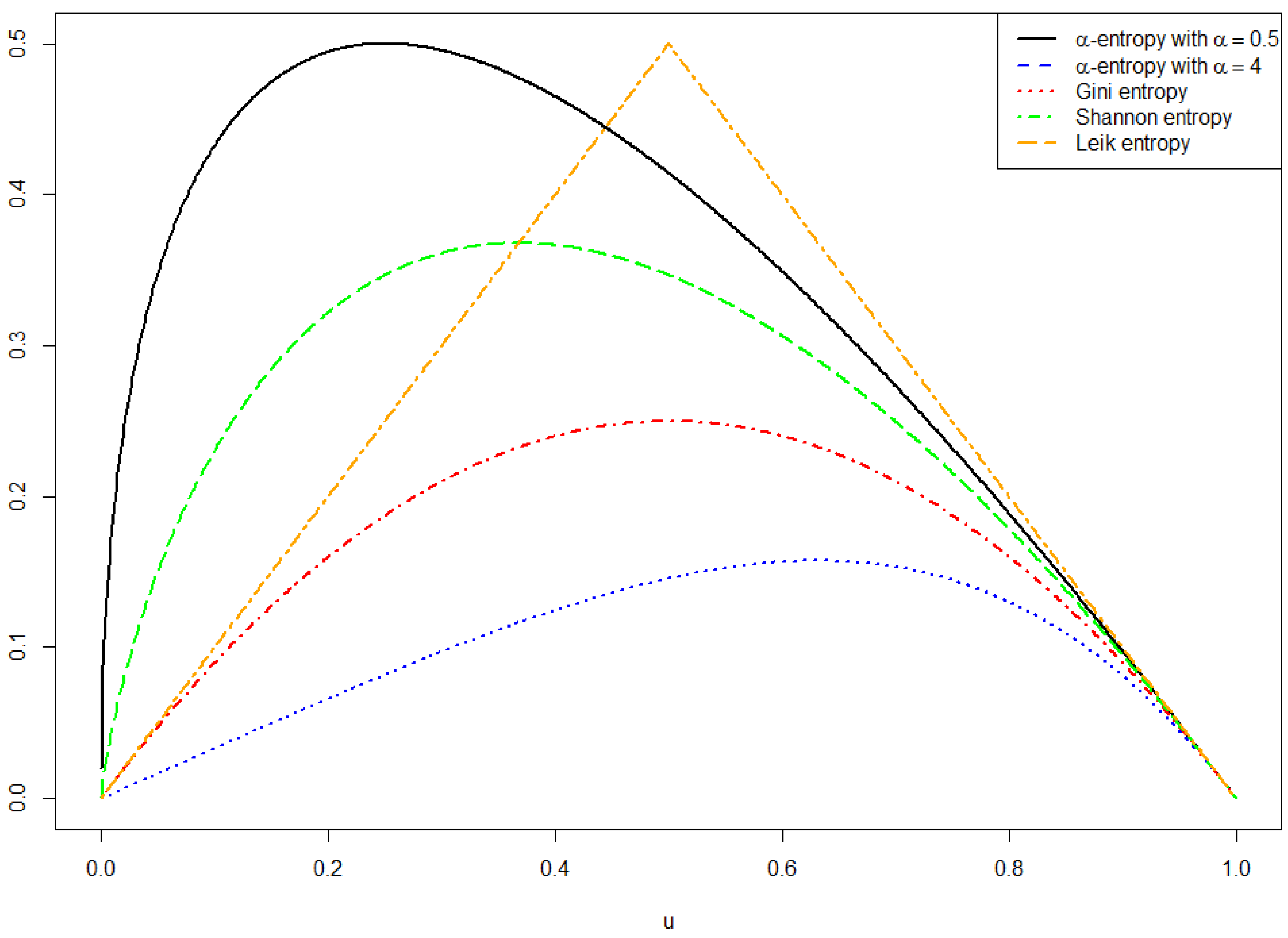
Figure 2.
Several entropy generating functions φ derived from the generalized maximum entropy (ME) principle.
Figure 2.
Several entropy generating functions φ derived from the generalized maximum entropy (ME) principle.

Figure 3.
φ-regression fit for the number of calls in the “telephone” data set.

Figure 4.
, for the standard Gaussian and the Student-t distribution.

© 2016 by the authors; licensee MDPI, Basel, Switzerland. This article is an open access article distributed under the terms and conditions of the Creative Commons Attribution (CC-BY) license (http://creativecommons.org/licenses/by/4.0/).
Share and Cite
MDPI and ACS Style
Klein, I.; Mangold, B.; Doll, M. Cumulative Paired φ-Entropy. Entropy 2016, 18, 248. https://doi.org/10.3390/e18070248
AMA Style
Klein I, Mangold B, Doll M. Cumulative Paired φ-Entropy. Entropy. 2016; 18(7):248. https://doi.org/10.3390/e18070248
Chicago/Turabian StyleKlein, Ingo, Benedikt Mangold, and Monika Doll. 2016. "Cumulative Paired φ-Entropy" Entropy 18, no. 7: 248. https://doi.org/10.3390/e18070248
Note that from the first issue of 2016, this journal uses article numbers instead of page numbers. See further details here.