Analysis of the Chaotic Behavior of the Lower Hybrid Wave Propagation in Magnetised Plasma by Hamiltonian Theory

Abstract

The Hamiltonian character of the ray tracing equations describing the propagation of the Lower Hybrid Wave (LHW) in a magnetic confined plasma device (tokamak) is investigated in order to study the evolution of the parallel wave number along the propagation path. The chaotic diffusion of the “time-averaged” parallel wave number at higher values (with respect to that launched by the antenna at the plasma edge) has been evaluated, in order to find an explanation of the filling of the spectral gap (Fisch, 1987) by “Hamiltonian chaos” in the Lower Hybrid Current Drive (LHCD) experiments (Fisch, 1978). The present work shows that the increase of the parallel wave number $n_{\parallel }$ due to toroidal effects, in the case of the typical plasma parameters of the Frascati Tokamak Upgrade (FTU) experiment, is insufficient to explain the filling of the spectral gap, and the consequent current drive and another mechanism must come into play to justify the wave absorption by Landau damping. Analytical calculations have been supplemented by a numerical algorithm based on the symplectic integration of the ray equations implemented in a ray tracing code, in order to preserve exactly the symplectic character of a Hamiltonian flow.

1. Introduction

Electromagnetic waves in the Lower Hybrid (LH) range of frequencies have long been used as an efficient way of generating a non-inductive current in magnetically-confined plasma (tokamak) [1,2]. The problem of describing the propagation of Lower Hybrid Waves (LHW) in such kind of confined plasma has been studied intensively during the last few decades, and simplified models, based on the Wentzel–Kramers–Brillouin (WKB) approximation, have been used because of the easier numerical and analytical implementation with respect to the more sophisticated Vlasov–Maxwell full system. In fact, the ray tracing technique, based on the WKB expansion of the wave equation [3,4,5,6,7,8], allows one to study the propagation (and the absorption) of the LHW in such plasma, by taking into account the toroidal geometry of the tokamak. The ray-tracing equations are formally the Hamilton equations of a mechanical system in which the roles of the momentum and position are assumed by wave vector and position, and the Hamiltonian is the dispersion relation, which correlates (ω, $\overrightarrow{k}$) to (t, $\overrightarrow{r}$), time and space. If the LHW is launched by an antenna, located at the plasma edge, and the condition of Landau absorption is not fulfilled inside the plasma, the wave remains trapped without absorption in the confined plasma. As an example, when the parallel (to the confining magnetic field) wave number ($n_{\parallel }=c/\omega k_{\parallel }$) of the launched wave satisfies the inaccessibility condition ($n_{\parallel }<n_{\parallel c}$), the wave remains trapped in a thin toroidal layer at the plasma edge bouncing back and forth for a long time; another example is when, due to the low temperature of the plasma, the wave bounces from the center (geometrical reflection) to the edge (cutoff) in a sort of multi-pass regime. This regime was proposed by Bonoli and Englade [6] in order to explain the filling of the spectral gap in the LHW absorption, by invoking a simple linear mechanism. The filling of the spectral gap is, in fact, the physical explanation of the fact that the high phase velocity (lowest launched parallel wave number compatible with the accessibility) slows sufficiently (increase of the parallel wave number) during the propagation to match the Landau absorption mechanism $n_{\parallel }>\alpha /\sqrt{T_e}$, where α is a number that can vary from five to seven and $T_e$ (the electron temperature) is expressed in $KeV$ [9]. The increase of the wave number, however, is not the only ingredient that allows an efficient current drive and improves the current drive efficiency; it is necessary that the width of the wave spectrum $\mathrm{\Delta }{n}_{\parallel }$, which is very narrow at the antenna and centered on $n_{\parallel 0}$ (as low as possible compatible with accessibility), becomes broader and, in the zone of the plasma-wave interaction, spans a large part of the resonant velocity space ($v_{\parallel }=c/n_{\parallel }$) from almost three- to six-times the thermal electron velocity. The up-shift and the broadening of the $n_{\parallel }$ spectrum is a very fast phenomenon, and it is related to the wave propagation time, which for the LH is very close to the propagation time of the light. This means that the wave propagating without absorption in the tokamak plasma (due to the high phase velocity and low temperature) can experience several radial reflections before being absorbed on the quasi-linear time scale (${\tau }_{ql}\approx v_{the}^2/D_{ql}$) if the spectral gap is fulfilled by the ray dynamics. Beyond this simple linear approach for solving the filling of the spectral gap, several mechanisms other than that delineated above have been invoked to solve this paradox in the LH absorption. Most of them are related to the nonlinear interaction between the wave and the plasma at the edge, as the Parametric Decay Instability (PDI) proposed in [10,11] by Porkolab, useful to explain the density limit for LHCD, and in [12,13,14] as proposed to explain, via nonlinear wave-plasma interaction at the edge, the filling of the spectral gap without invoking the dynamical effects on the ray trajectories. Other explanations are based on the wave scattering from density fluctuation [15,16,17]; collisional absorption has been invoked in [18,19]; some other mechanisms are based on the inclusion of the diffraction effects in the wave propagation, which are disregarded in the usual WKB approximation, and are included by a full wave approach in the solution of the Maxwell equation [20,21] or, keeping the WKB approximation, by the beam tracing approach [22,23]. Scattering of LHW by drift wave turbulence, in addition to the toroidal effects, was also proposed in [24].

In this paper, we come back to the multi-pass approach and, by exploiting the Hamiltonian character of the ray tracing equations, we try to study the dynamical evolution of the rays in the case of long integration time (when the ray experienced a large number of radial reflections): in this situation, the nonlinear effects which stem out from the nonlinear ray equations (Hamilton equations) can play a role in the chaotic evolution of the dynamical system. This chaotic evolution of the trajectory can be associated with a chaotic diffusion of the “parallel wave number”. This kind of approach in the spectral gap explanation had been proposed several years ago in [25] by Wersinger et al. to explain the ergodization (and the consequent detrapping) of the ray trajectories due to the toroidicity (two degrees of freedom effects on the Hamilton equations) of some PDI-generated LHW trapped in the low density plasma region; successively, this approach has been used by Bonoli and Ott [17] to explain the propagation (due to toroidal effects) of the inaccessible part of the launched LHW spectrum ($n_{\parallel }<n_{\parallel c}$) in conjunction with the scattering of density fluctuations. A full numerical approach has been adopted in [26,27,28] to show that the spectral gap was apparently filled by Hamiltonian chaos that diffuses energy towards higher parallel wave numbers. In particular, in [27,28], a ray-tracing multi-pass code was coupled to a 1D Fokker–Planck calculation, to incorporate not only the $n_{\parallel }$ diffusion, but also the modification of the electron distribution function. Obviously, when the Landau damping is very strong (in the case of first pass absorption), the wave spectrum behaves regularly without stochastic diffusion [28].

Further applications of this stochastic approach to the LHW propagation can be found in [29,30,31] in which various mechanisms breaking the cylindrical symmetry, like toroidicity and magnetic ripple, can induce chaotic evolution of the trajectories and can help with bridging the spectral gap. However, when applying the rigorous Hamiltonian formalism as developed in [31], taking as Hamiltonian the electrostatic dispersion relation and trying to give some analytical insight of the nonlinear LH ray dynamics, the conclusion is that the LH propagation in cylindrical plasmas with magnetic ripple is generally regular. In [30], instead, the filling of the spectral gap was reached by chaotic diffusion due to the presence, in the electromagnetic case, of a separatrix.

In a general system of coordinates without symmetries, the Hamilton equations describe a dynamical system with three degrees of freedom (dof), and in the case of an axisymmetric plasma (tokamak), the system is two dof. In this context, the “Hamiltonian” is essentially the cold electromagnetic dispersion relation, and the canonical conjugated variables are the wave vector and the position. The system is non-integrable, if a second constant of motion other than the energy is missing, and the chaotic diffusion of the time-averaged parallel wave number towards higher values has been evaluated to corroborate or disprove the filling of the spectral gap in the LHW absorption mechanism. Analytical calculations (see, for example, Cardinali and Romanelli in [32]) have demonstrated that the non-integrability is essentially due to the geometry or any other mechanism breaking the symmetry of the system (magnetic ripple, density and magnetic fluctuations). 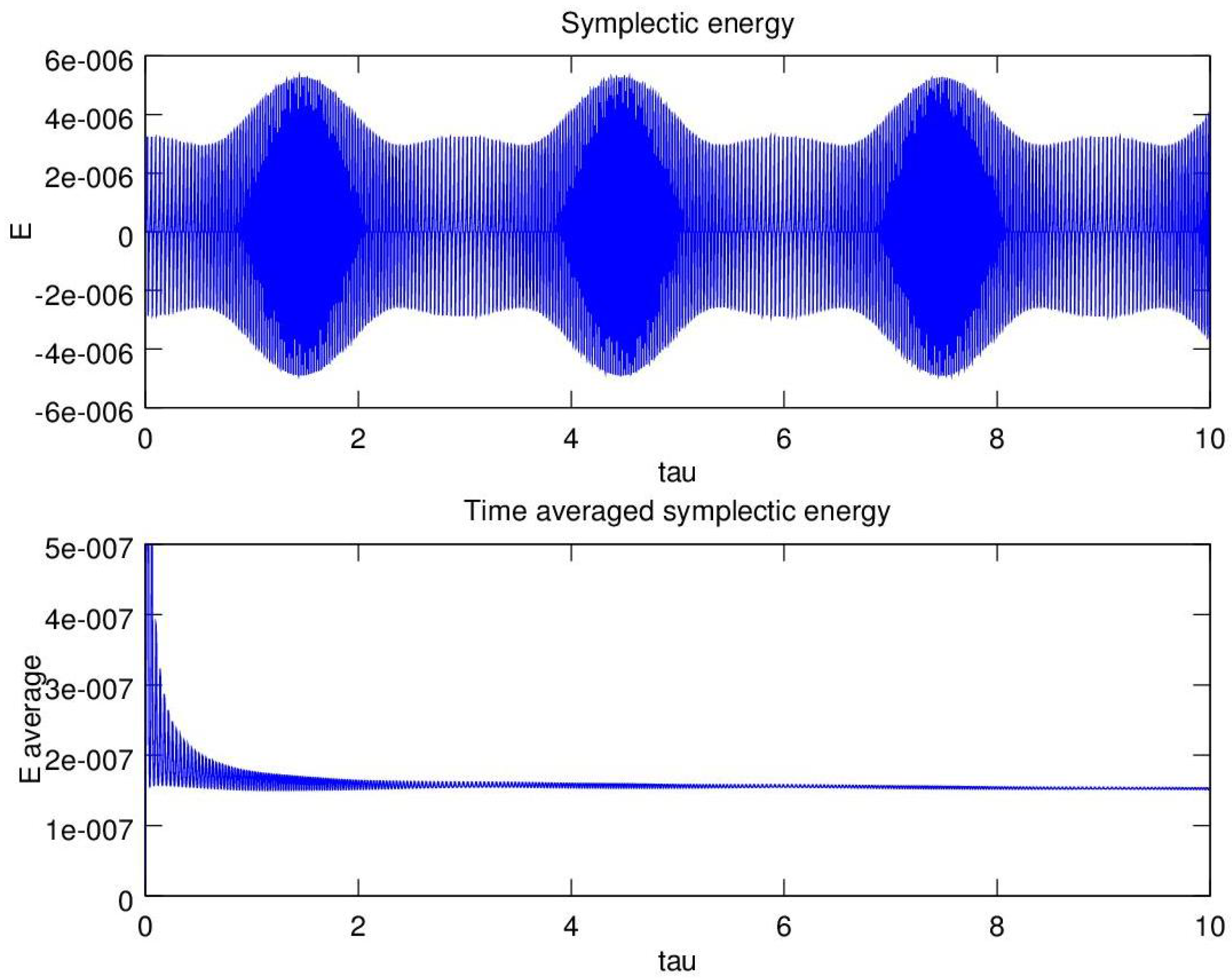As long as toroidicity can be considered a perturbation of the cylindrical geometry (small inverse aspect ratio $ϵ\ll 1$), the non-integrable Hamiltonian system can be analytically studied by the perturbation theory [33] where the zero-order Hamiltonian $H_0$ is one dof, while the perturbed Hamiltonian $H_1$ is two dof. Moreover, the non-integrability of the physical system can also affect the evolution of a bundle of trajectories when describing several modes radiated by the antenna (spectrum). For a chaotic system, the spreading of the trajectories is exponential (Lyapunov exponents): this leads to a destruction of the wave spectrum in a relatively short time. Numerical analysis by means of a symplectic algorithm [34], implemented in a ray-tracing code, support the analytical considerations. It is worth remarking here that accurate symplectic algorithms have been recently implemented (see, for example, [35,36]), and they have been applied to the study of charged particles’ motion in a plasma (see [37]).

Attempts to analytically solve the Hamilton equations have already been made, even if in a different way [38]. The dispersion relation of the cold plasma in cylindrical coordinates strictly resembles the Hamiltonian of an isotropic 3D harmonic oscillator, so we studied the effect of toroidal geometry as a small perturbation of the original integrable system. To this end, we made use of canonical perturbation theory [33,39] to find an approximate solution to the problem in terms of the canonical action-angle variables. The fact that the toroidal effects can be considered as perturbations of the integrable system is made possible by the smallness of the inverse aspect ratio ϵ, which can be taken as a perturbative parameter. The results of the canonical perturbation theory and the related numerical integration of the rays suggest that the increase in the average value of $n_{\parallel }$ is limited to low values, so there must be another mechanism that comes into play to fill the spectral gap and justify the results obtained on Frascati Tokamak Upgrade (FTU) in the Lower Hybrid Current Dive (LHCD) experiments [40,41]. Nevertheless, in our study, we have performed a complete scan in plasma and geometrical parameters (inverse aspect ratio) to establish the transition to the chaotic behavior of the trajectories. In particular, we have pointed out the role of the density, plasma current and toroidal magnetic field, which act like “energy” in the context of the Hamiltonian formulation, as well as the aspect ratio, which plays the role of the perturbative parameter in our analytical calculation. Several attempts have been made by other groups to take into account the nonlinear mode coupling, which is responsible for a significant spectral broadening [42], and so, justify the wave absorption due to the quasilinear effects of the broadened wave spectrum for higher components of the parallel wave number.

The paper is organized as follows. In Section 2, the analysis of the simplified electromagnetic dispersion relation (Hamiltonian) is performed. In Section 3, simplified expressions for the Hamiltonian of the slow and the fast branches are deduced in cylindrical geometry. In Section 4, the effect of the toroidal geometry is assessed and treated like a perturbation of the one dof cylindrical Hamiltonian. In Section 5, we remind about the basic concepts of the canonical perturbation theory. In Section 6, we remind about the fundamental result of the Kolmogorov–Arnold–Moser (KAM) theory, and we draw our conclusions about the absence of resonances in our system. In Section 7, extensive numerical results are given for the plasma parameters of the FTU tokamak, whose magnetic surfaces are circularly shaped. In Section 8, we compare our results to those of a few previous works, where important conclusions on the existence of an upper limit to $n_{\parallel }$ were drawn. 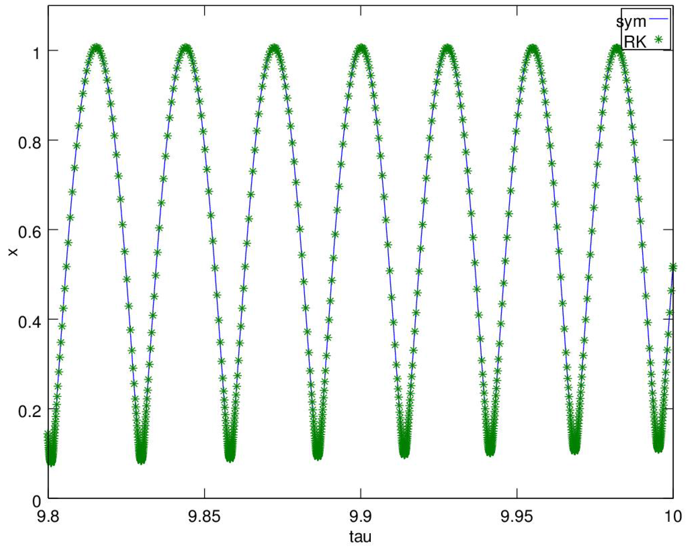In Section 9, we provide a few words about the symplectic algorithm that we used, and we compare it to the more commonly-used Runge–Kutta integrator. Finally, in Section 10, conclusions are drawn, and the results are discussed.

2. The Electromagnetic Dispersion Relation as a Hamiltonian Function

The starting point is the cold electromagnetic wave equation for the harmonic electric field perturbation ($\overrightarrow{E}(\overrightarrow{q},t)=\overrightarrow{E}(\overrightarrow{q})e^{i\omega t}$) suitable to describe the propagation of LHW (GHz range of frequencies) in magnetically-confined plasmas:

$$\nabla \wedge \nabla \wedge \overrightarrow{E}(\overrightarrow{q})+\frac{{\omega }^2}{c^2}\underline{\underline{ϵ}}(\overrightarrow{p},\overrightarrow{q})·\overrightarrow{E}(\overrightarrow{q})=\gamma (\overrightarrow{p},\overrightarrow{q})\overrightarrow{E}(\overrightarrow{q})$$

(1)

where $\overrightarrow{p},\overrightarrow{q}$ are the wave vector and position, respectively, $\underline{\underline{ϵ}}(\overrightarrow{p},\overrightarrow{q})$ is the Hermitian part of the cold plasma dielectric tensor, $\gamma (\overrightarrow{p},\overrightarrow{q})$ is the damping factor (Landau damping) related to the anti-Hermitian part of the dielectric tensor and $\overrightarrow{E}(\overrightarrow{q})$ is the harmonic electric field, which depends on position $\overrightarrow{q}$. Equation (1) can be solved by the WKB expansion, assuming the following form for the electric field:

$$\overrightarrow{E}(\overrightarrow{q})={\overrightarrow{E}}_0(\overrightarrow{q})e^{i{h}^{-1}S(\overrightarrow{q})}$$

(2)

where ${\overrightarrow{E}}_0(\overrightarrow{q})$ is the slowly-varying amplitude, $S(\overrightarrow{q})$ is the phase that varies on a smaller length-scale and $h^{-1}=\omega a/c\ll 1$ is the WKB expansion parameter (a is the plasma minor radius). Applying the form just chosen for the electric field to Equation (1) and using toroidal coordinates $\overrightarrow{q}=(r,\theta ,\varphi )$ and $\overrightarrow{p}=(p_r,p_{\theta },p_{\varphi })$, we obtain to the lowest order the following dispersion equation for the conjugated variables $\overrightarrow{p},\overrightarrow{q}$:

$$H(q_i,p_i)=A(r,\theta ,p_{\theta },p_{\varphi })p_r^4+B(r,\theta ,p_{\theta },p_{\varphi })p_r^2+C(r,\theta ,p_{\theta },p_{\varphi })=0$$

(3)

where:

$$\begin{array}{cc}& A=S\hfill \\ & B=2S{k}_{\chi }^2+(P+S)k_{\parallel }^2+\frac{{\omega }^2}{c^2}[D^2-S(P+S)]\hfill \\ & C=S{k}_{\chi }^4+(P+S)k_{\chi }^2{k}_{\parallel }^2+\frac{{\omega }^2}{c^2}[D^2-S(P+S)]k_{\chi }^2-2\frac{{\omega }^2}{c^2}PS{k}_{\parallel }^2+\frac{{\omega }^4}{c^4}P(S^2-D^2)+P{k}_{\parallel }^4\hfill \end{array}$$

(4)

S, D and P are the elements of the cold dielectric tensor in Stix notation [43]; $\overrightarrow{p}=\nabla S(\overrightarrow{q})$, ${\widehat{B}}_{\theta }$ and ${\widehat{B}}_{\varphi }$ are the poloidal and toroidal magnetic fields (normalized to $\left|B\right|$); $R=R_0(1+r/R_{0}cos\theta )$ is the metric factor; $R_0$ is the major radius of the torus. In Equation (3), we used the conjugated variables position and momentum ($\overrightarrow{q},\overrightarrow{p}$) instead of position an wave vector ($\overrightarrow{r},\overrightarrow{k}$) for analogy with the corresponding mechanical system. We have introduced the wave vectors ${\overrightarrow{k}}_{\chi }$ and ${\overrightarrow{k}}_{\parallel }$, such that:

$${\overrightarrow{k}}_{\chi }={\widehat{B}}_{\theta }\frac{p_{\varphi }}{R}-{\widehat{B}}_{\varphi }\frac{p_{\theta }}{r}{\overrightarrow{k}}_{\parallel }={\widehat{B}}_{\theta }\frac{p_{\theta }}{r}+{\widehat{B}}_{\varphi }\frac{p_{\varphi }}{R}$$

(5)

Equation (3) represents the Hamilton–Jacobi equation for the generating function $S(\overrightarrow{q})$, once the substitution $\overrightarrow{p}=\nabla S(\overrightarrow{q})$ has been made, and $H(\overrightarrow{q},\overrightarrow{p})$ is the corresponding Hamiltonian. Note that the Hamiltonian does not depend on the toroidal angle φ because of the axisymmetry of the system: this means that the toroidal wave number is a constant. Since the Hamiltonian is formally written as in Equation (3), the “energy” of the system is implicitly contained in the function $H(q_i,p_i,E)=0$, and it includes the macroscopic plasma parameters as central density, plasma current, toroidal magnetic field, etc., which are fixed at the beginning of the calculation. Changing these parameters means to change the “energy” injected in the analogous mechanical system (mutatis mutandis). Now, using the fact that $m_e/m_i\ll 1$ and ${\mathrm{\Omega }}_{ci}\ll \omega \ll {\mathrm{\Omega }}_{ce}$ (LH range of frequencies) and considering the following ordering for the Stix elements of the dielectric tensor, $S=O(1)$; $D=O({(m_e/m_i)}^{-1/4})$; $P=O({(m_e/m_i)}^{-1})$, we can write the following simplified Hamiltonian for the slow and fast branches of the LHW:

$$H(q_i,p_i)=p_r^2+k_{\chi }^2+\frac{P}{2S}\left[k_{\parallel }^2-\frac{{\omega }^2}{c^2}S\right]\left\{1\pm \sqrt{1-\frac{{\omega }^4}{c^4}\frac{4D^{2}S}{\left|P\right|{\left[k_{\parallel }^2-\frac{{\omega }^2}{c^2}S\right]}^2}}\right\}=0$$

(6)

By substituting in Equation (6) the following simplified expressions for S, D and P:

$$\begin{array}{cc}& S\approx 1\hfill \\ & D\approx -\frac{{\omega }_{pe0}^2}{\omega {\mathrm{\Omega }}_{ce0}}\left(1-\alpha \frac{r^2}{a^2}\right)\left(1+\frac{r}{R_0}cos\theta \right)\hfill \\ & P\approx 1-\frac{{\omega }_{pe0}^2}{{\omega }^2}\left(1-\alpha \frac{r^2}{a^2}\right)\hfill \end{array}$$

(7)

and considering that the following inequality holds:

$$\frac{{\omega }^4}{c^4}\frac{4D^{2}S}{\left|P\right|{\left[k_{\parallel }^2-\frac{{\omega }^2}{c^2}S\right]}^2}\ll 1$$

(8)

when:

$$k_{\parallel }>k_{\parallel crit}\approx \frac{\omega }{c}\left(\sqrt{S}+\frac{\left|D\right|}{\sqrt{\left|P\right|}}\right)$$

(9)

we have finally the simplified and decoupled Hamiltonian related to the slow wave branch (sign “+”):

$$H{(q_i,p_i)}_s\approx p_r^2+{\left({\widehat{B}}_{\theta }\frac{p_{\varphi }}{R}-{\widehat{B}}_{\varphi }\frac{p_{\theta }}{r}\right)}^2+\left[1-\frac{{\omega }_{pe0}^2}{{\omega }^2}\left(1-\alpha \frac{r^2}{a^2}\right)\right]{\left({\widehat{B}}_{\theta }\frac{p_{\theta }}{r}+{\widehat{B}}_{\varphi }\frac{p_{\varphi }}{R}\right)}^2$$

(10)

and the fast branch (sign “−”):

$$H{(q_i,p_i)}_f\approx p_r^2+{\left({\widehat{B}}_{\theta }\frac{p_{\varphi }}{R}-{\widehat{B}}_{\varphi }\frac{p_{\theta }}{r}\right)}^2-\frac{{\omega }^4}{c^4}\frac{\frac{{\omega }_{pe0}^4}{{\omega }^2{\mathrm{\Omega }}_{ce0}^2}{\left(1-\alpha \frac{r^2}{a^2}\right)}^2}{{\left({\widehat{B}}_{\theta }\frac{p_{\theta }}{r}+{\widehat{B}}_{\varphi }\frac{p_{\varphi }}{R}\right)}^2}{\left(1+\frac{r}{R_0}cos\theta \right)}^2$$

(11)

The slow branch is often called also “electrostatic”, because it is essentially longitudinal; for this reason, in the following, we will use alternatively one or the other name to refer to this mode of propagation. Note that in Equation (7), we have assumed a parabolic profile for the density, as has been done in [31], which is consistent with the experimental data collected on FTU during LHCD; $\alpha =1-n_{edge}/n_0$ is a parameter that accounts for the edge density, while the toroidal magnetic field varies as $B(r,\theta )=R_0{B}_0/R$. The subscript “0” in the expressions for the plasma and cyclotron frequencies refers to the central density $n_{e0}$ and magnetic field $B_0$. R depends on r and θ through:

$$R=R_0\left(1+\frac{r}{R_0}cos\theta \right)$$

(12)

In the case where Equation (8) is not satisfied in some points inside the plasma, the slow and fast branches of the dispersion relation are coupled, and the Hamiltonian, which must be considered, is the following:

$$\begin{array}{cc}\hfill H{(q_i,p_i)}_{coup}=p_r^2+& {\left({\widehat{B}}_{\theta }\frac{p_{\varphi }}{R}-{\widehat{B}}_{\varphi }\frac{p_{\theta }}{r}\right)}^2+\frac{1}{2}\left[1-\frac{{\omega }_{pe0}^2}{{\omega }^2}\left(1-\alpha \frac{r^2}{a^2}\right)\right]\left[{\left({\widehat{B}}_{\theta }\frac{p_{\theta }}{r}+{\widehat{B}}_{\varphi }\frac{p_{\varphi }}{R}\right)}^2-\frac{{\omega }^2}{c^2}\right]\hfill \\ & ·\left\{1\pm \sqrt{1-4\frac{{\omega }^4}{c^4}\frac{\frac{{\omega }_{pe0}^2}{{\mathrm{\Omega }}_{e0}^2}\left(1-\alpha \frac{r^2}{a^2}\right)}{{\left[{\left({\widehat{B}}_{\theta }\frac{p_{\theta }}{r}+{\widehat{B}}_{\varphi }\frac{p_{\varphi }}{R}\right)}^2-\frac{{\omega }^2}{c^2}\right]}^2}{\left(1+\frac{r}{R_0}cos\theta \right)}^2}\right\}=0\hfill \end{array}$$

(13)

where the subscript “coup” means “coupled”.

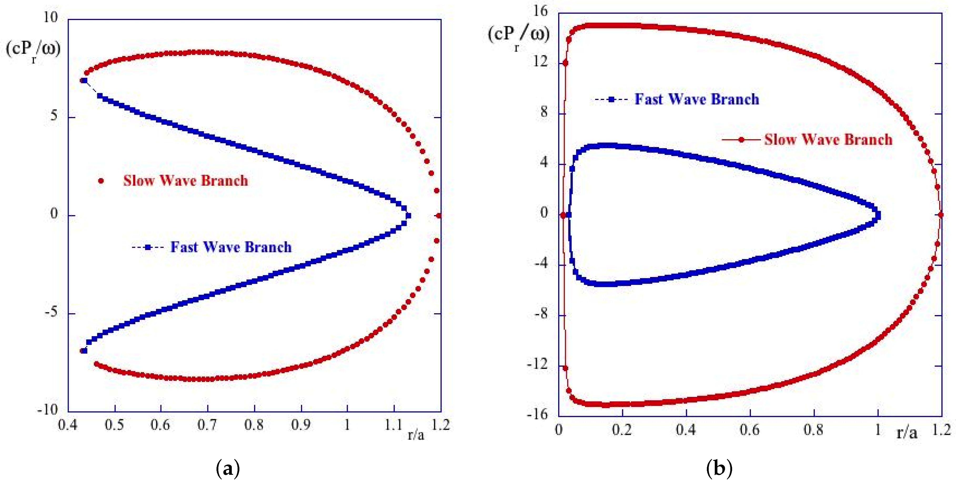
3. The Integrable Cylindrical Limit

Due to the independence of the toroidal angle φ, the Hamiltonians in Equations (10), (11) and (13) represent a system with two dof, in which $p_{\varphi }$ (conjugated to φ) is a constant of motion. This means that the system is not integrable if there is not a second constant of motion in addition to the energy, and in principle, it is possible to deal with Hamiltonian chaos. In order to explore this possibility in the frame of perturbation theory and successively with the numerical integration on Hamilton equations by a symplectic algorithm, we take the cylindrical limit: $R\to R_0$ for $ϵ=r/R_0\to 0$, where ϵ is the inverse aspect ratio, that can be considered as the natural expansion parameter when applying the perturbation theory. The Hamiltonian Equations (10) and (11) can be cast in the following forms for the slow wave branch:

$$H{(r,p_r)}_s\equiv p_r^2+\frac{p_{\theta }^2}{r^2}+{\kappa }_0\frac{r^2}{a^2}=E_0$$

(14)

and for the fast branch:

$$H{(r,p_r)}_f\equiv p_r^2+\frac{p_{\theta }^2}{r^2}+{\kappa }_1\frac{r^2}{a^2}+{\kappa }_2\frac{r^4}{a^4}=E_1$$

(15)

where E and κ are the equivalent of the energy and the elastic constants in the analogue mechanical system and whose dimensions are $l^{-2}$. These quantities are defined below, and as is possible to notice, they depend on the plasma, machine and antenna parameters: density, current, magnetic field, major and minor radius, frequency and launched poloidal and toroidal wave numbers.

$$\begin{array}{cc}& E_0=\frac{1}{R_0^2}\frac{{\omega }_{pe0}^2}{{\omega }^2}{\left(\frac{p_{\theta }}{q_a}+p_{\varphi }\right)}^2-\frac{1}{R_0^2}\left(\frac{p_{\theta }^2}{q_a^2}+p_{\varphi }^2\right)\hfill \\ & {\kappa }_0=\frac{1}{R_0^2}\left[{\left(\frac{a{p}_{\varphi }}{R_0{q}_a}\right)}^2+\alpha \frac{{\omega }_{pe0}^2}{{\omega }^2}{\left(\frac{p_{\theta }}{q_a}+p_{\varphi }\right)}^2\right]\hfill \\ & E_1=2\frac{p_{\theta }{p}_{\varphi }}{R_0^2{q}_a}+R_0^2\frac{{\omega }_{pe0}^4{\omega }^2}{c^4{\mathrm{\Omega }}_{e0}^2}{\left(\frac{p_{\theta }}{q_a}+p_{\varphi }\right)}^{-2}\hfill \\ & {\kappa }_1=\frac{1}{R_0^2}{\left(\frac{a{p}_{\varphi }}{R_0{q}_a}\right)}^2+2\alpha R_0^2\frac{{\omega }_{pe0}^4{\omega }^2}{c^4{\mathrm{\Omega }}_{e0}^2}{\left(\frac{p_{\theta }}{q_a}+p_{\varphi }\right)}^{-2}\hfill \\ & {\kappa }_2=-{\alpha }^2{R}_0^2\frac{{\omega }_{pe0}^4{\omega }^2}{c^4{\mathrm{\Omega }}_{e0}^2}{\left(\frac{p_{\theta }}{q_a}+p_{\varphi }\right)}^{-2}\hfill \end{array}$$

(16)

In the coupled case, Equation (13) can be written as:

$$H{(r,p_r)}_{coup}=p_r^2+\frac{p_{\theta }^2}{r^2}+{\kappa }_3\frac{r^2}{a^2}+E_2\pm \left[E_3+{\kappa }_4\frac{r^2}{a^2}\right]\sqrt{1+4\frac{{\kappa }_2}{\alpha {\kappa }_0}\left(1-\alpha \frac{r^2}{a^2}\right)}$$

(17)

where we have defined the new constants:

$$\begin{array}{cc}& E_2=\frac{1}{2R_0^2}{\left(\frac{p_{\theta }}{q_a}+p_{\varphi }\right)}^2-\frac{1}{2R_0^2}\frac{{\omega }_{pe0}^2}{{\omega }^2}{\left(\frac{p_{\theta }}{q_a}+p_{\varphi }\right)}^2-2\frac{p_{\theta }{p}_{\varphi }}{R_0^2{q}_a}\hfill \\ & E_3=E_2+2\frac{p_{\theta }{p}_{\varphi }}{R_0^2{q}_a}\hfill \\ & {\kappa }_3=\frac{1}{R_0^2}{\left(\frac{a{p}_{\varphi }}{R_0{q}_a}\right)}^2+\frac{1}{2R_0^2}\alpha \frac{{\omega }_{pe0}^2}{{\omega }^2}{\left(\frac{p_{\theta }}{q_a}+p_{\varphi }\right)}^2\hfill \\ & {\kappa }_4={\kappa }_3-\frac{1}{R_0^2}{\left(\frac{a{p}_{\varphi }}{R_0{q}_a}\right)}^2\hfill \end{array}$$

(18)

It can be seen easily that ${\kappa }_3+{\kappa }_4={\kappa }_0$ and $E_2+E_3\approx -E_0$. Using these relationships, it is easy to find the previous expression Equations (14) and (15) by using the appropriate approximations. The argument of the square root in Equation (17) can be written also as:

$$\begin{array}{c}\hfill \sqrt{1+4\frac{{\kappa }_2}{\alpha {\kappa }_0}\left(1-\alpha \frac{r^2}{a^2}\right)}=\sqrt{\frac{r_c^2}{a^2-r_c^2}}\sqrt{\frac{r^2}{r_c^2}-1}\end{array}$$

(19)

where:

$$r_c^2=\frac{a^2}{\alpha }\left\{1-\frac{c^4}{{\omega }^4}\frac{{\mathrm{\Omega }}_{e0}^2}{4{\omega }_{pe0}^2}\frac{1}{R_0^2}\left[\frac{1}{R_0^2}{\left(\frac{p_{\theta }}{q_a}+p_{\varphi }\right)}^2-\frac{{\omega }^2}{c^2}\right]\right\}$$

(20)

is the “confluence” point, where the mode conversion occurs. The phenomenon of mode conversion is the process through which a wave, which is launched on one propagation branch from the edge of the plasma, converts to the other branch of propagation at an intermediate point, where the argument of the square root becomes zero. The wave then propagates outward till it reaches the cutoff and is again reflected inward, and the process repeats ad infinitum.

Due to the poloidal symmetry, $p_{\theta }$ is now a constant of motion. In the derivation of Equations (14), (15) and (17), we have considered ${\widehat{B}}_{\varphi }\approx 1$ and ${\widehat{B}}_{\theta }/{\widehat{B}}_{\varphi }=r/(R_0{q}_a)=O(\eta )$, ($\eta \sim {ϵ}^2\ll 1$), and $q_a$ is the safety factor at $r=a$. The Hamiltonians of the decoupled slow and fast branches are perfectly integrable because they are one dof and are similar to the Hamiltonian of a body subject to a central elastic force in polar coordinates. To proceed further, we have to find the change from the original variables to the action-angle variables to apply the canonical perturbation theory. The change of variables is formally given by:

$$\begin{array}{cc}& J=\frac{1}{2\pi }\oint pdq\hfill \\ & \mathrm{\Phi }=\frac{\partial S}{\partial J}=\int pdq\hfill \end{array}$$

(21)

where the integration path in the first integral is the path followed by the unperturbed system in its orbit. Since the mechanical analogue of the system we are studying is the isotropic oscillator, in order to calculate the action variable, we simply need to integrate between the turning points of the radial motion. The Hamiltonian of the slow wave branch is biquadratic in r, which means that we can find easily the inversion points for the radial motion by solving a quadratic equation for $r^2$. The Hamiltonian of the fast wave branch instead is a sixth-degree polynomial in r, which means that, to find the inversion points of the radial motion, we should solve a third-order equation in $r^2$. This is possible, but the formulas are very complicated, so we preferred here to simplify the Hamiltonian of the fast wave branch by neglecting the term ${\kappa }_2{r}^4$. The reasons for this choice are the following: first of all, by numerically integrating the ray equations in cylindrical geometry, we find that the phase portrait of the fast wave branch looks very similar in shape to the phase portrait of the slow wave, which means that somehow, their dynamics are similar; then, the coefficients ${\kappa }_1$ and ${\kappa }_2$ are approximately equal in absolute value, but for a factor two in the expression of ${\kappa }_1$, which makes it larger; finally, the coordinate r is always smaller than the minor radius a, so that $r^4/a^4\ll r^2/a^2$. In conclusion, we can write:

$$H{(r,p_r)}_f\approx p_r^2+\frac{p_{\theta }^2}{r^2}+{\kappa }_1\frac{r^2}{a^2}=E_1$$

(22)

Explicit calculations made on Equation (14) and on Equation (22) show that the cutoff of the slow wave branch is located at $r\approx a$, while for the fast wave branch is located at $r\approx a/\sqrt{2}$ because of the factor two in the $k_1$ coefficient. This is a further clue that our assumption is correct.

After several passages, reported in Appendix A, the final expressions for the action-angle variables for the slow wave are:

$$\begin{array}{cc}& J=\frac{E_0}{4\sqrt{A}}-\frac{p_{\theta }}{2}\hfill \\ & \mathrm{\Phi }=arcsin\left[\frac{2A{r}^2-E_0}{\sqrt{E_0^2-4A{p}_{\theta }^2}}\right]\hfill \end{array}$$

(23)

where $A={\kappa }_0/a^2$. The corresponding variables for the fast wave can be obtained by the substitution $E_0\to E_1$ and ${\kappa }_0\to {\kappa }_1$. In the cylindrical case, $p_{\theta }$ is a constant of motion. Inverting the expressions for Φ and using the expression for J, we obtain:

$$r^2=\frac{1}{\sqrt{A}}\left(2J+p_{\theta }+2\sqrt{J^2+J{p}_{\theta }}sin\mathrm{\Phi }\right)=\chi +\xi sin\mathrm{\Phi }$$

(24)

where we have defined the functions:

$$\chi =\frac{2J+p_{\theta }}{\sqrt{A}}\xi =\frac{\sqrt{J^2+J{p}_{\theta }}}{\sqrt{A}}$$

(25)

From Equation (14), we can write the Hamiltonian in terms of the canonical variables:

$$H_0=2\sqrt{A}(2J+p_{\theta })=E_0$$

(26)

where $H_0$ is the unperturbed, integrable Hamiltonian. The unperturbed frequencies of the integrable system can be obtained as:

$${\omega }_{0r}=\frac{\partial H_0}{\partial J}=4\sqrt{A}{\omega }_{0\theta }=\frac{\partial H_0}{\partial p_{\theta }}=2\sqrt{A}$$

(27)

Again, ${\kappa }_0$ and $E_0$ hold for the slow wave, while for the fast wave, we have to make the substitutions $E_0\to E_1$ and ${\kappa }_0\to {\kappa }_1$. We see from Equation (27) that the frequency ratio is ${\omega }_{0r}/{\omega }_{0\theta }=2$.

4. Effect of the Toroidal Geometry: Non-Integrable System

Our purpose in this and in the following sections is to study the Hamiltonian of the LHW in the decoupled case by the canonical perturbation theory. First, we have to write the complete Hamiltonian in the form:

$$H(r,\theta ,p_r,p_{\theta },p_{\varphi })=H_0(r,p_r,p_{\varphi })+ϵH_1(r,\theta ,p_r,p_{\theta },p_{\varphi })$$

(28)

where $H_0$ is the unperturbed Hamiltonian, $H_1$ is the perturbation and ϵ is the small expansion parameter. In our case, $H_0(r,p_r,p_{\varphi })$ is given by Equation (26), and the perturbation is given by the θ-dependent parts of the complete Hamiltonian proportional to the inverse aspect ratio $ϵ=a/R_0$. By expanding Equations (10) and (11) to first order in ϵ, we find, for the perturbation $H_1$, the following expressions:

$$H_{1s}=-2cos\theta \left\{\left[{\left(\frac{a{p}_{\varphi }}{R_0^2{q}_a}\right)}^2+\alpha \frac{{\omega }_{pe0}^2}{{\omega }^2}\left(\frac{p_{\theta }{p}_{\varphi }}{R_0^2{q}_a}+\frac{p_{\varphi }^2}{R_0^2}\right)\right]\frac{r^3}{a^3}-\frac{{\omega }_{pe0}^2}{{\omega }^2}\left(\frac{p_{\theta }{p}_{\varphi }}{R_0^2{q}_a}+\frac{p_{\varphi }^2}{R_0^2}\right)\frac{r}{a}\right\}$$

(29)

for the slow branch and:

$$\begin{array}{cc}\hfill H_{1f}& \approx 2cos\theta \left\{\left[\frac{p_{\theta }{p}_{\varphi }}{R_0^2{q}_a}-2R_0^2{\left(\frac{p_{\theta }}{q_a}+p_{\varphi }\right)}^{-2}\frac{{\omega }^2{\omega }_{pe0}^4}{c^4{\mathrm{\Omega }}_{e0}^2}\right]\frac{r}{a}-\right.\hfill \\ & \left.-\left[{\left(\frac{a{p}_{\varphi }}{R_0^2{q}_a}\right)}^2-4\alpha R_0^2{\left(\frac{p_{\theta }}{q_a}+p_{\varphi }\right)}^{-2}\frac{{\omega }^2{\omega }_{pe0}^4}{c^4{\mathrm{\Omega }}_{e0}^2}\right]\frac{r^3}{a^3}-{\alpha }^2{R}_0^2{\left(\frac{p_{\theta }}{q_a}+p_{\varphi }\right)}^{-2}\frac{{\omega }^2{\omega }_{pe0}^4}{c^4{\mathrm{\Omega }}_{e0}^2}\frac{r^5}{a^5}\right\}\hfill \end{array}$$

(30)

for the fast branch. Since $\alpha \approx 1$, ${(a{p}_{\varphi }/(R_0^2{q}_a))}^2\ll ({\omega }_{pe0}^2/{\omega }^2)(p_{\varphi }^2/R_0^2)$ and ${(a{p}_{\varphi }/(R_0^2{q}_a))}^2\ll ({\omega }_{pe0}^4{\omega }^2/(c^4{\mathrm{\Omega }}_{e0}^2))(R_0^2/p_{\varphi }^2)$, several simplifications can be done so that Equations (10) and (11) become:

$$H{(r,p_r,\theta ,p_{\theta })}_s\approx p_r^2+\frac{p_{\theta }^2}{r^2}+{\kappa }_0\frac{r^2}{a^2}+2{\kappa }_0\left(\frac{r}{a}-\frac{r^3}{a^3}\right)ϵcos\theta =E_0$$

(31)

$$H{(r,p_r,\theta ,p_{\theta })}_f\approx p_r^2+\frac{p_{\theta }^2}{r^2}+{\kappa }_1\frac{r^2}{a^2}+2{\kappa }_1\left(-\frac{r}{a}+2\frac{r^3}{a^3}-\frac{r^5}{a^5}\right)ϵcos\theta =E_1$$

(32)

${\kappa }_0$, ${\kappa }_1$, $E_0$ and $E_1$ have been defined above (Equation (16)).

5. Canonical Perturbation Theory

To proceed in the canonical perturbation theory, we have to find the generating function $S_1$ for the new variables $J_1$, ${\mathrm{\Phi }}_1$, $p_{\theta 1}$, ${\theta }_1$, such that the complete Hamiltonian depends only on the actions. Here, we will remind about the basic principles of the theory as stated in [33,39]. The generating function must fulfill the following equation:

$${\omega }_0^{\alpha }\frac{\partial S_1}{\partial {\mathrm{\Phi }}_{\alpha }}=〈V〉-V$$

(33)

where ${\omega }_0^{\alpha }$ are the unperturbed frequencies, V is the perturbation and $〈V〉$ is its average over the angle variables. To solve this equation, let us call $\tilde{V}=V-〈V〉$ and expand $S_1$ and $\tilde{V}$ in a Fourier series over the angles:

$$S_1=\sum _m{S}_{1m}{e}^{im·\mathrm{\Phi }};\tilde{V}=\sum _m{\tilde{V}}_m{e}^{im·\mathrm{\Phi }}$$

(34)

so that the solution of Equation (33) becomes:

$$S_1=i\sum _{m\alpha }\frac{V_{m\alpha }}{m_{\alpha }{\omega }^{\alpha }}{e}^{i{m}_{\alpha }{\mathrm{\Phi }}^{\alpha }}$$

(35)

and the new variables are given by:

$$\begin{array}{cc}\hfill J_1& =J+ϵ\partial S_1/\partial \mathrm{\Phi }{\mathrm{\Phi }}_1=\mathrm{\Phi }-ϵ\partial S_1/\partial J\hfill \\ \hfill p_{\theta 1}& =p_{\theta }+ϵ\partial S_1/\partial \theta {\theta }_1=\theta -ϵ\partial S_1/\partial p_{\theta }\hfill \end{array}$$

(36)

Since $S_1$ presents the denominators $m·{\omega }_0$, canonical perturbation theory fails in the presence of resonances, that is when $m·{\omega }_0\approx 0$. This is the famous problem of small denominators, found for the first time by Poincaré [44], which is fundamental for KAM theory. Here, $m·{\omega }_0\approx 0$ is a short notation for:

$$m_1{\omega }_{01}+m_2{\omega }_{02}\approx 0$$

(37)

meaning that it is a scalar product between an integer vector and a vector whose components are the unperturbed frequencies.

6. KAM Theory and Its Consequences

Before proceeding to apply the theory we have just delineated to our particular case, we have to remind about the results of the KAM theory. When the problem of small denominators first came out in the study of dynamical systems, the first hypothesis that was formulated was that any system would be unstable with respect to arbitrarily small perturbations due to the inevitable presence of resonances in the form $m·{\omega }_0=0$. In fact, rationals are dense in reals, so that there would be a resonant torus arbitrarily close to any orbit in the phase-space of the system, which would cause the series of the Fourier coefficients to diverge. Successively, thanks to the studies of Kolmogorov [45], Arnold [46] and Möser [47], the understanding of the problem improved. In fact, the new result obtained by the three authors we have just quoted is that the condition of non-resonance:

$$m·{\omega }_0\ne 0\forall m$$

(38)

should be substituted with:

$$m·{\omega }_0>\frac{\gamma }{{\left|m\right|}^{\nu }}\forall m$$

(39)

for the series of coefficients to converge. Here, γ is a constant of the order of ϵ and $\nu >N-1$, with N the number of dof of the system. Equation (39) is also called the “Diophantine condition”, and its meaning is that the ratio between the different frequencies, associated with the different dof, is sufficiently irrational. That said, we are looking for resonances between the frequencies of the system in order to determine its stability with respect to small perturbations.

To apply the perturbation theory to the Hamiltonian $H_1$, we have to calculate first its Fourier coefficients. We notice immediately that the expansion has infinite terms due to the particular form of the perturbation, so we should in principle express it as an infinite series. To calculate this expansion, we consider that:

$$r={(\chi +\xi sin\mathrm{\Phi })}^{1/2}\approx {\chi }^{1/2}{(1+sin\mathrm{\Phi })}^{1/2}{r}^3={(\chi +\xi sin\mathrm{\Phi })}^{3/2}\approx {\chi }^{3/2}{(1+sin\mathrm{\Phi })}^{3/2}$$

(40)

because $\chi \approx \xi$. The functions ${(1+sin\mathrm{\Phi })}^{1/2}$ and ${(1+sin\mathrm{\Phi })}^{3/2}$ have an exact expansion in Fourier series:

$$\begin{array}{cc}& {(1+sin\mathrm{\Phi })}^{1/2}=\frac{2\sqrt{2}}{\pi }\left[1+\frac{1}{3}sin\mathrm{\Phi }+\cdots \right]\hfill \\ & {(1+sin\mathrm{\Phi })}^{3/2}=\frac{8\sqrt{2}}{\pi }\left[\frac{1}{3}+\frac{1}{5}sin\mathrm{\Phi }+\cdots \right]\hfill \end{array}$$

(41)

so in principle, we could consider as many Fourier components as we want, but it is not necessary. In fact, we saw in the previous sections that the ratio of unperturbed frequencies is ${\omega }_{0r}/{\omega }_{0\theta }=2$, so a resonance between them cannot occur, since the Fourier expansion of $cos\theta$ has only the term $m=1$. The same argument holds for the perturbation to the fast branch, where an additional $r^5$ term appears. In fact, the resonance condition between the frequencies becomes:

$$|m_{0\theta }|{\omega }_{0\theta }=\left|m_{0r}\right|{\omega }_{0r}$$

(42)

Since ${\omega }_{0r}=2{\omega }_{0\theta }$, this would require a component $m_{0\theta }=2$ in the Fourier expansion, which is not present at this order of approximation. Taking the exact expansion of the metric coefficient:

$$\frac{1}{1+ϵxcos\theta }=\sum _{n=0}^{\infty }{(-1)}^n{(ϵxcos\theta )}^n$$

(43)

we can recover all of the terms in the Fourier expansion relative to the angle θ, but expanding this expression in powers of ϵ means going beyond the first order in the perturbation theory. Such a thing is beyond the aim of this paper, so we will not go any further in the analytical calculations.

7. Numerical Results

The analytical considerations have been supplemented with the numerical integration of ray trajectories by means of a symplectic algorithm (see Appendix B). The position and the wave vector (momentum) evolve according to the Hamilton equations:

$$\begin{array}{cc}& \dot{r}=\frac{\partial H}{\partial p_r},\dot{p_r}=-\frac{\partial H}{\partial r}\hfill \\ & \dot{\theta }=\frac{\partial H}{\partial p_{\theta }},\dot{p_{\theta }}=-\frac{\partial H}{\partial \theta }\hfill \\ & \dot{\varphi }=\frac{\partial H}{\partial p_{\varphi }},\dot{p_{\varphi }}=-\frac{\partial H}{\partial \varphi }\hfill \end{array}$$

(44)

and the equation for the time variable $\dot{t}=-\partial H/\partial \omega$, where it is possible to notice that in the two dof problem $p_{\varphi }=const$, and φ is ignorable. Applying them to the Hamiltonian Equation (3), we obtain the trajectories in the phase-space of the system, in particular those corresponding to the main variables, that is r and $p_r$, or the corresponding adimensional variables $x=r/a$ and $p_x=c/\omega p_r$. Before proceeding to perform a parametric study of the Hamilton Equation (44), it is worth solving them in the cylindrical limit $ϵ\to 0$. 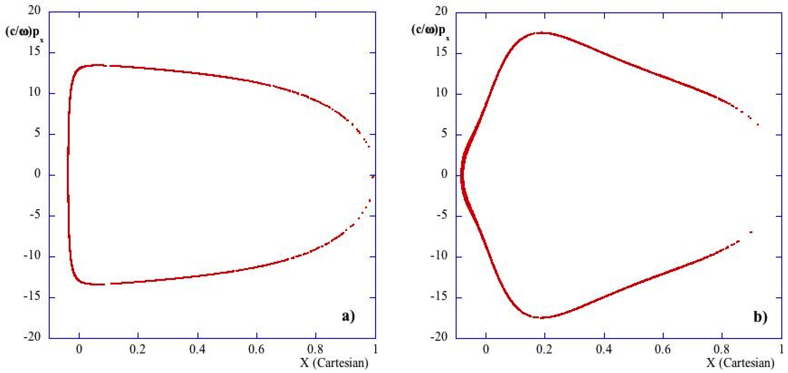The equation system (Equation (44)) reduces to a simple quadrature. The phase portrait of the fast and slow branches in cylindrical geometry is shown in Figure 1 for the coupled ($n_{\parallel }=n_{\parallel crit}$ in some points inside the plasma column) and the decoupled case ($n_{\parallel }>n_{\parallel crit}$ everywhere in the plasma). The points on the surface of the section are aligned because the cylindrical case is integrable. The difference between the coupled and the decoupled case and its effect on ray propagation have been stressed by Bizarro et al. (see, for example, Figure 6 of [31]).

In the coupled case, we see the mode conversion phenomenon taking place at the point where the propagation passes from one branch to the other in the previously-defined “confluence” point. When including the toroidicity through the small expansion parameter ϵ, the dynamics of the system changes. 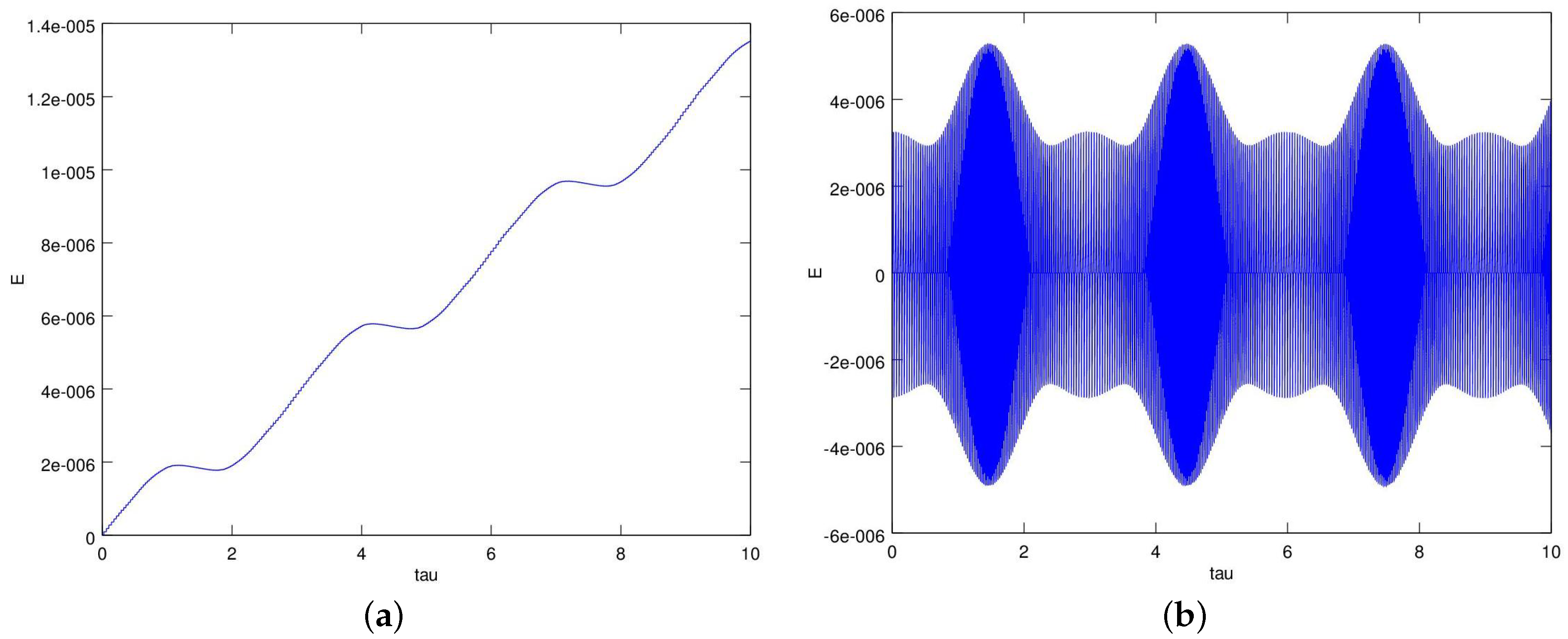As we could expect from considerations of Hamiltonian dynamics, the trajectories are not closed like in the cylindrical case at one dof (in the ($p_r-r$) space) due to the non-integrability of the system (Figure 2a). In fact, the point of closest approach to $x\approx 0$ varies in time due to the variation of $p_{\theta }$. In Figure 2b, the evolution of the parallel wave number is shown vs. the time (in $\mu s$) for the same FTU plasma parameters of Figure 2a. On the same plot, the accessible (critical) wave number $n_{\parallel crit}$ (solution of the equations $B^2-4AC=0$ (Equations (3) and (4))) is also displayed clearly showing that the mode conversion does not occur for this choice of plasma and antenna parameters. It is worth noting that $n_{\parallel }$ is an oscillating function of the propagation time, which looks very regular with minima and maxima that are $n_{\parallel min}=1.9$ and $n_{\parallel max}=3.5$. Moreover, its time-average along the trajectory gives $〈n_{\parallel }〉=2.7$. Here, the time-average is performed over the entire integration time.

Although the Hamiltonian we are dealing with in the numerical code corresponds to the full electromagnetic dispersion relation, here, we present some results of the numerical integration of the ray-tracing equations in absence of mode conversion, that is for a value of the parallel wave number $n_{\parallel }$, such that the wave propagates always on the same branch (the slow one, in our case). It is worth noting that in the case $n_{\parallel }\gg n_{\parallel crit}$, the Hamiltonian of Equation (3) reduces to a much simpler Hamiltonian that corresponds to the electrostatic limit of the dispersion relation. For these simulations, we chose the FTU typical plasma and antenna parameters, that is a central density in the range $n_{e0}={10}^{13}÷{10}^{14}{\text{cm}}^{-3}$, inverse aspect ratio $ϵ=0.3$, toroidal magnetic field on axis $B_0=4÷8T$, plasma current $I_p=0.3÷1MA$, corresponding to $3<q_a<10$, LH frequency $f=8GHz$, launched parallel wave number $n_{\parallel }=1.32÷2.42$ (following the antenna phasing) (see [41]).

Looking at the analytical Hamiltonian of Equation (31), which strongly resembles that of the elastic pendulum (in the mechanical analogues) and that has been treated in [48,49], we perform here a numerical study to establish the emergence of the chaos in the ray trajectories’ integration as a function not only of the aspect ratio (which is breaking the cylindrical symmetry), but also as a function of the energy and elastic constant of the system ($E_0$ and ${\kappa }_0$ in Equation (16)). These quantities in the plasma are essentially depending on the main plasma and antenna parameters: that is, central density $n_{e0}$, toroidal magnetic field $B_0$, plasma current $q_a$, toroidal wave number $p_{\varphi }$, LH frequency ω; for this reason, we integrate the ray trajectories by changing parametrically one plasma (or antenna) parameter keeping fixed the others and fixing in this study the initial conditions for the set of equations that are defining the ray-tracing equations. We choose to represent the Poincaré sections in Cartesian variables ($X,P_X$) instead of the (normalized) cylindrical variables ($x,p_x$) for practical reasons. The first parametric study is related to the variation of the central plasma density from $n_{e0}=5\times {10}^{13}{\text{cm}}^{-3}$ to $n_{e0}=1.5\times {10}^{14}{\text{cm}}^{-3}$ (note that a realistic range of values for FTU is included between $n_{e0}={10}^{13}{\text{cm}}^{-3}$ up to $n_{e0}={10}^{14}{\text{cm}}^{-3}$) keeping fixed the plasma current $I_p=0.6MA$ ($q_a\approx 4$), the magnetic field $B_0=6T$, $p_{\varphi }=354.14$ (which corresponds to $n_{\parallel }\approx 1.8$, the peak value of the power spectrum of the grill antenna). 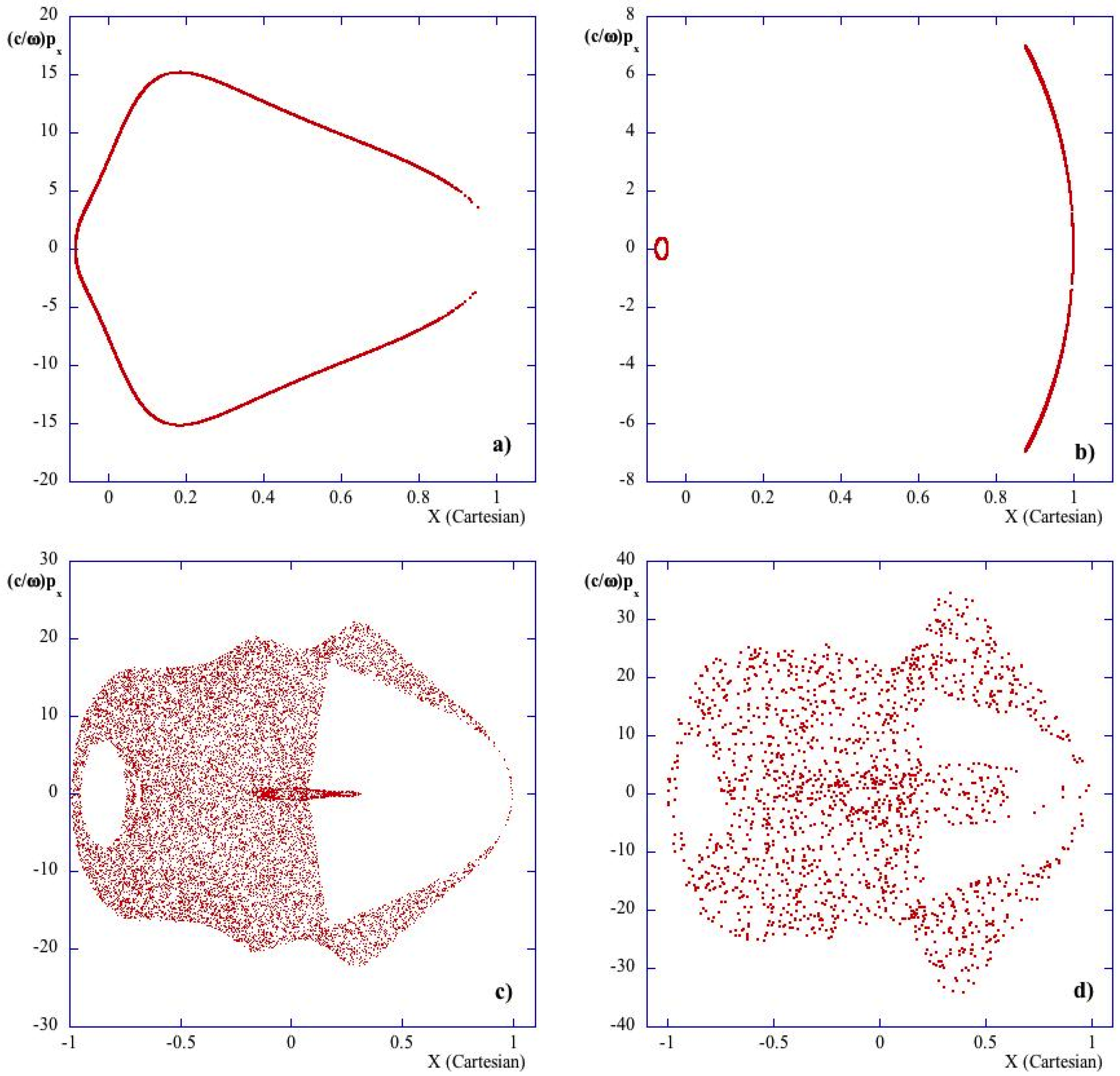In the set of figures (Figure 3), we present the Poincaré map for four different levels of central density ($(a)$ $5\times {10}^{13}{\text{cm}}^{-3}$; $(b)$ $8\times {10}^{13}{\text{cm}}^{-3}$; $(c)$ $9\times {10}^{13}{\text{cm}}^{-3}$; $(d)$ $1.5\times {10}^{14}{\text{cm}}^{-3}$) corresponding to four increasing levels of energy (cf. Equation (14)). The ray-tracing integration starts with the following initial conditions: $r=a$, $\theta =0$ (injection from the low-field side and on the equatorial plane of the torus); $p_r=0.6256{\text{cm}}^{-1}$ is calculated from the dispersion relation at the plasma boundary (solution of the biquadratic Equation (3) with the sign + (slow wave branch)); and finally, $p_{\theta }=0$, which is essentially the wave number of the LHw launched by a grill whose vertical dimension is much greater then the horizontal one $L_y\gg L_z$. The concept behind the Poincaré section is explained in [49]. The procedure starts with the choice of a value for the energy (and of course, of all of the other parameters of the system). This reduces the number of independent coordinates of our system from four ($r,\theta ,p_r,p_{\theta }$) to three ($r,\theta ,p_r$). If an independent conserved quantity other than the energy exists, this would reduce the number of independent variables to two. 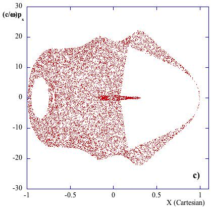In this case, if we take one of the three variables to be constant (θ), the points where the trajectory intersects the so-defined plane will form a well-defined curve. If such a conserved quantity does not exist, the constraint disappears, and the intersection points tend to densely fill this plane, which we will call the surface of the section or the Poincaré section. This is the case for chaotic motion. The mapping that takes us from a point on the surface of the section to the next is called a Poincaré map. This method provides a direct visualization of the regularities or irregularities of a given trajectory in the phase space of a system. As can be seen from the sequence of Figure 3, the Poincaré section ($P_X-X$) is regular up to a density level $8\times {10}^{13}{\text{cm}}^{-3}$; after this threshold, the ray dynamics becomes chaotic. For density lower then $8\times {10}^{13}{\text{cm}}^{-3}$ (which is the usual range of operating density in LHCD experiments), the dynamics is regular. From the numerical solution of Hamiltonian equations, it is also possible to study the variation of the parallel wave number, due to the variation of $p_{\theta }$. The variation we are looking for is an increase in the average value of $n_{\parallel }=c/\omega k_{\parallel }$, which would be responsible for the wave absorption by Landau damping on the electrons. The numerical results suggest that $p_{\theta }$ undergoes a small increase on average and so does $n_{\parallel }$. The increase in the time average $〈n_{\parallel }〉$ is limited enough to be incompatible with an efficient wave absorption by Landau damping, which requires a parallel wave number $n_{\parallel ELD}$, such that [9]:

$$n_{\parallel }>n_{\parallel ELD}=(5÷8)/\sqrt{T_{eKeV}}$$

(45)

(being $T_{e0}\approx 1-2KeV$ in the LH experiments on FTU [41]). In the reported cases of Figure 4, the time-averaged $n_{\parallel }$ is shown for cases of Figure 3a,b (without chaos), $〈n_{\parallel }〉=3.2$, $〈n_{\parallel }〉=2$, respectively, and for cases of Figure 3c,d (in presence of chaos), $〈n_{\parallel }〉=4.5$ and $〈n_{\parallel }〉=10.4$, respectively. The time evolution of the time-averaged parallel wave number was obtained by taking, for each instant τ, the average of $n_{\parallel }$ over the time interval τ:

$$〈n_{\parallel }(\tau )〉=\frac{1}{\tau }{\int }_0^{\tau }{n}_{\parallel }(t)dt$$

(46)

Only in the case of an unrealistic value of central density ($1.5\times {10}^{14}{\text{cm}}^{-3}$) and strongly chaotic behavior, the average parallel wave number is much higher than $n_{\parallel ELD}$.

The same calculation has been performed by keeping fixed the density (e.g., at $5\times {10}^{13}{\text{cm}}^{-3}$) and all of the other plasma and antenna parameters and varying the safety factor at the plasma boundary from $q_a=3$ up to $q_a=11$. This corresponds to considering a plasma current from $0.8MA$ up to $0.22MA$. In order to choose similar initial conditions for all of the runs, we are starting the rays very close to the cutoff density where $p_r\approx 0$. The results are shown in Figure 5 where a sequence of Poincaré plots is given for each value of $q_a$ ($q_a=(a)3; (b)5; (c)8; (d)9$). It seems that increasing $q_a$ (reducing the plasma current), a more irregular situation is met, although a strong chaotic dynamics can be excluded. This can be explained looking at Equation (16), which shows that the energy of the system is dominated essentially by the central density, and it is affected to a very limited extent by the plasma current ($q_a$). From a physical point of view, the increase in the energy of the system brings a stronger coupling between the slow and the fast branches of the LH dispersion relation. In our study, we have always considered the two branches as independent, but at higher density, they become closer, and in particular, the critical parallel wavenumber $n_{\parallel c}$ previously defined increases. This means that, even if the mode conversion phenomenon does not occur, the dynamics of the system must be described by the full electromagnetic dispersion relation Equation (13) instead of the two decoupled version Equations (10) and (11).

Despite the fact that a given tokamak (like FTU) has a fixed aspect ratio, we also made some Poincaré sections of the system to show how the dynamic behavior changes in the phase space increasing the value of the small expansion parameter ϵ starting from zero (cylindrical limit) to the real value of the FTU inverse aspect ratio for fixed plasma and antenna parameters. We recall that ϵ is the expansion parameter (see Section 4 and Section 5) that in our analytical approach is responsible for the breaking of the cylindrical symmetry and which possibly causes the ray dynamics to be chaotic. In Figure 6, we show the effect of the geometrical factor ϵ in the appearance/disappearance of chaos. 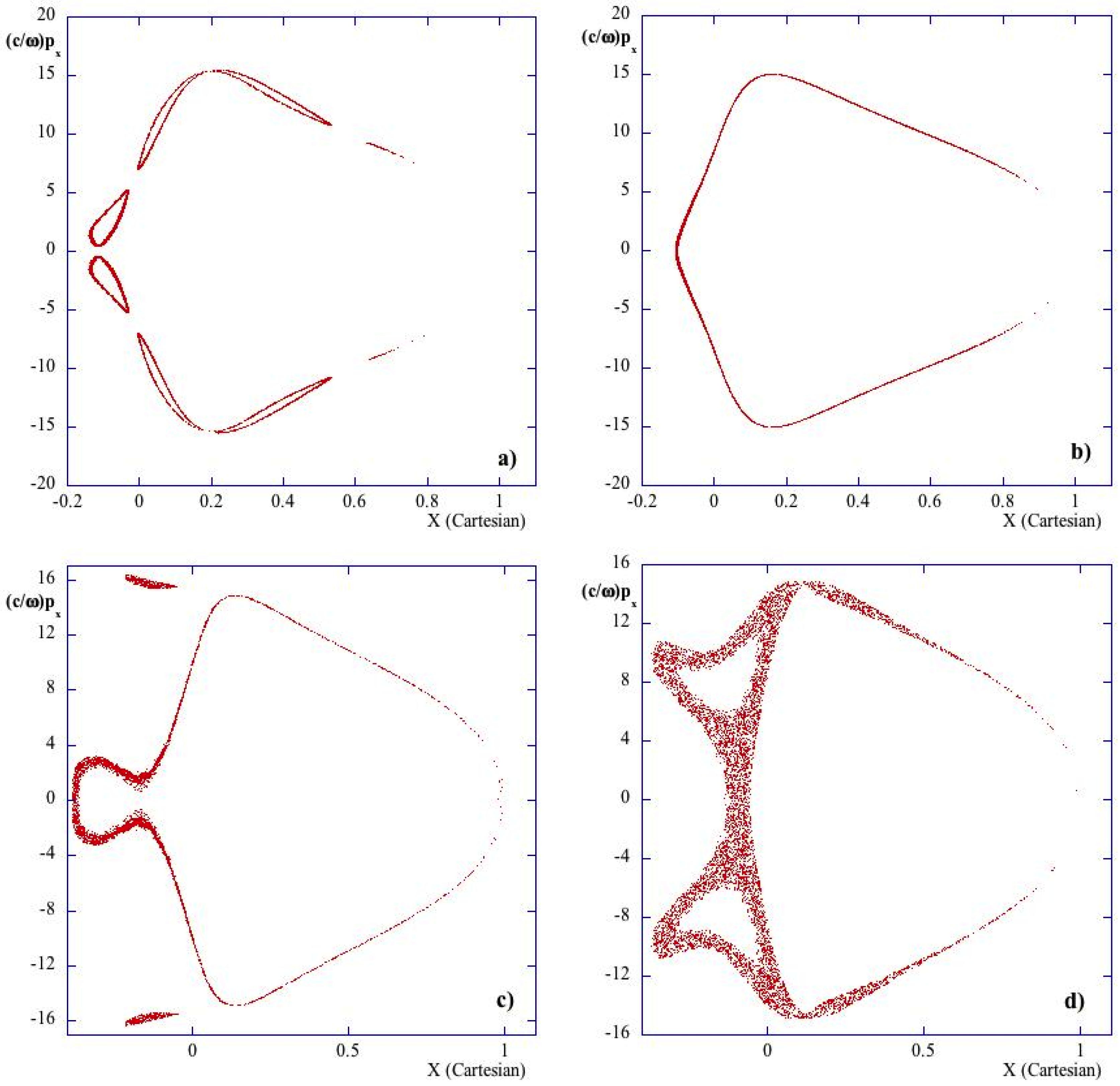We have plotted the Poincaré section for four different values of the inverse aspect ratio (ϵ = (a) 0.05; (b) 0.1; (c) 0.3; (d) 0.35) fixing the plasma parameters and the initial conditions.

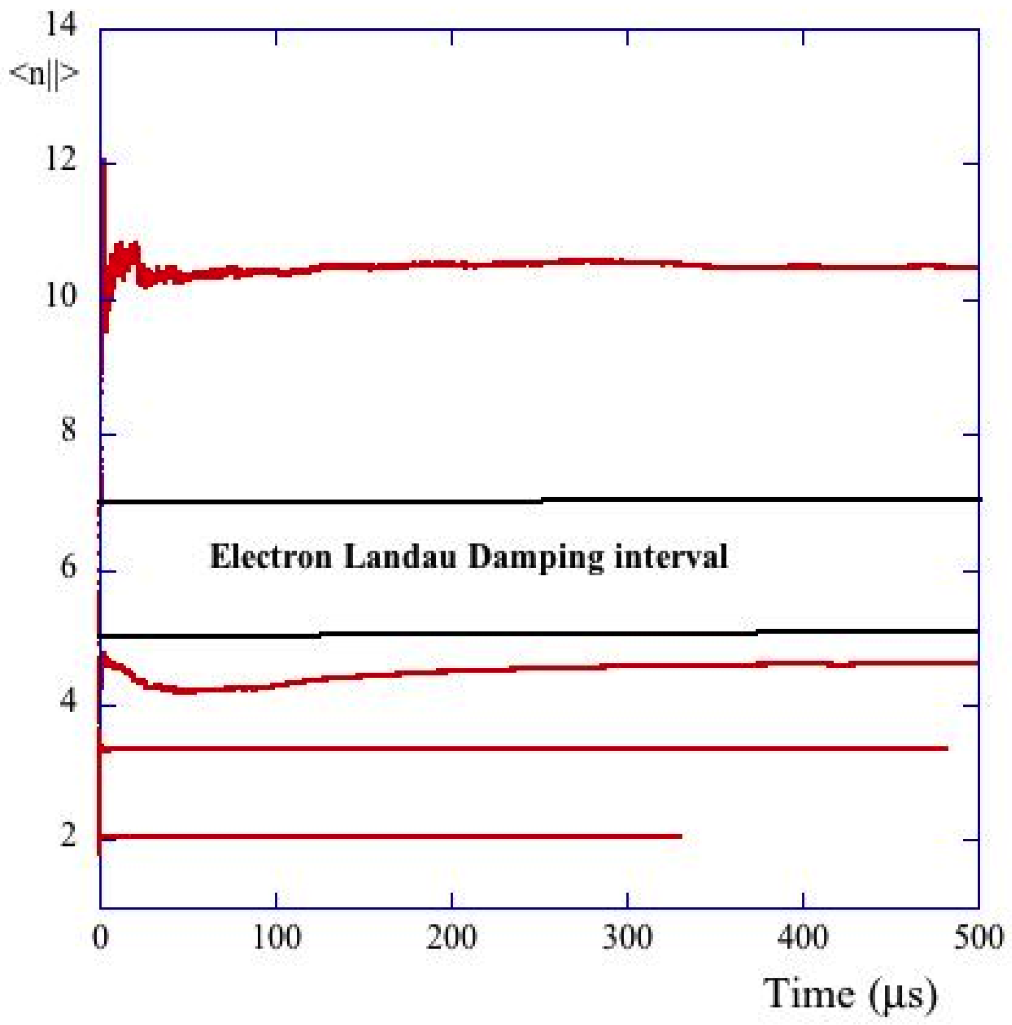
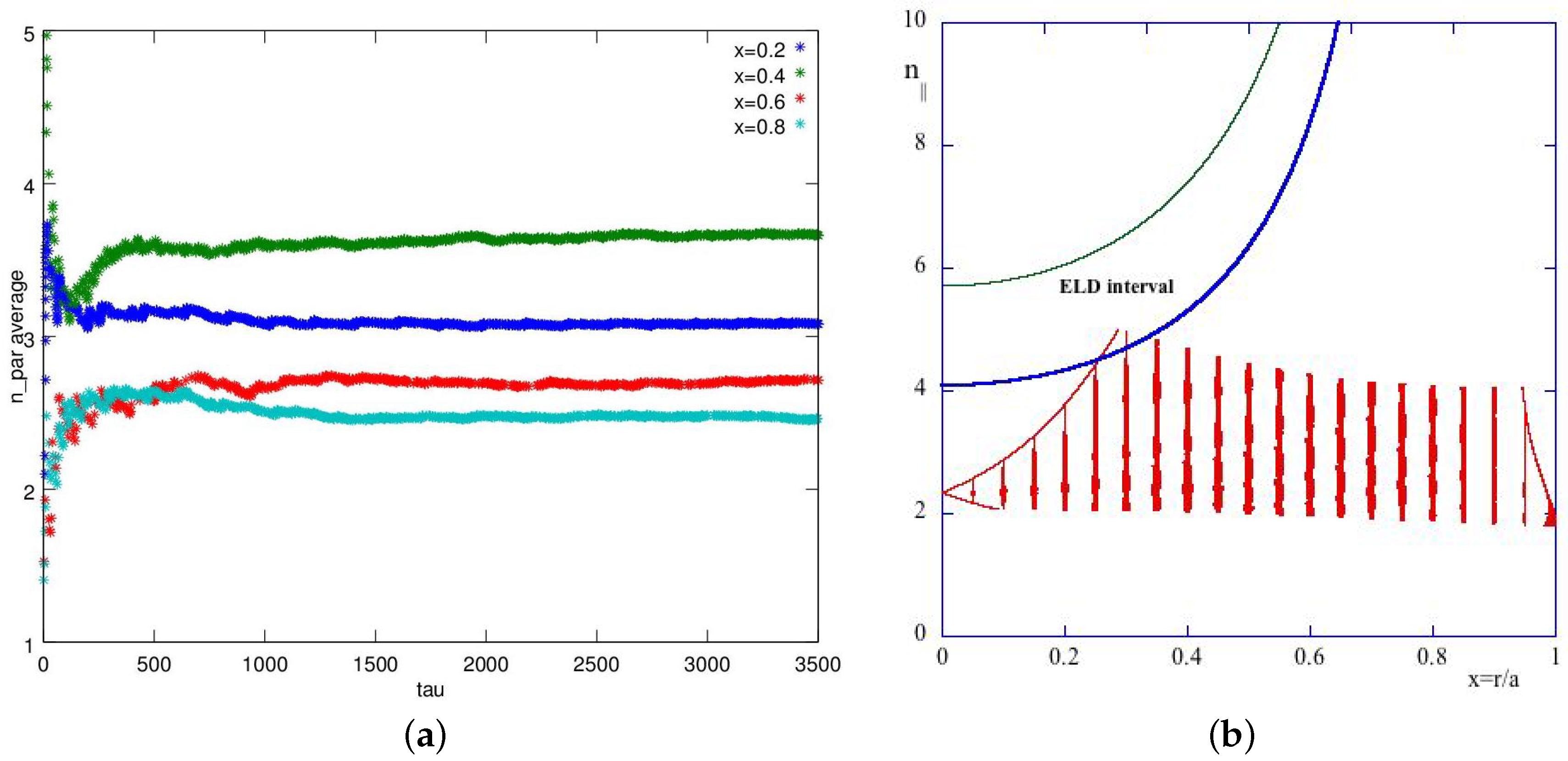
The $n_{\parallel }(\tau )$ evolution results in being a harmonic function of the time, when looking at its value on a magnetic surface ($r=const$), and the variation of its absolute value is contained in a boundary around an average value, which corresponds to that launched by the antenna and which is far too low to justify the filling of the spectral gap, which requires a local value as given in Equation (45). Thus, we checked the value of the parallel wave number in different radial positions, corresponding to different magnetic surfaces, to see whether the average value of $n_{\parallel }$ grows to the same value in all of the volume of the plasma or not. To this end, we took the value of $n_{\parallel }$ for different values of the radial coordinate, and then, we computed the arithmetic average, which is expressed with a formula very similar to Equation (46). In fact, unlike in Figure 4, here, we preferred to compute the arithmetic average of $n_{\parallel }$ over the number of crossings of the magnetic surfaces by the ray trajectory, which is more meaningful than the time average. The results, shown in Figure 7a, indicate that the parallel wave number remains limited to low values over all of the magnetic surfaces, even if the points relative to the very central regions and the boundary are very few, because the wave spends very little time there, and so, their importance for the wave absorption is negligible. We show in Figure 7b the range of $n_{\parallel }$ in different radial positions and the theoretical range suitable for Electron Landau Damping (ELD), delimited by the blue and green curves. We see that these curves are always higher than the values of $n_{\parallel }$ usually observed in the experiments performed on FTU. The red vertical bars correspond to the range of values of $n_{\parallel }$ for each different radial position, while the two lateral continuous lines are the upper bounds to the $n_{\parallel }$ upshifting. The plasma parameters used in this simulation are those of Figure 3a.

We also want to highlight the fact that, for the wave absorption, it is better to consider the average value of $n_{\parallel }$ instead of its instantaneous value, because the absorption process takes place on longer time scales than the wave propagation. We have seen however that the time-averaged $n_{\parallel }$ remains limited to low values, so there is no significative Landau damping anyway. Other mechanisms must come into play to fill the spectral gap: to remain in the ray-tracing framework, a valid possibility can be the effect of the magnetic ripple; in a more general approach, an important contribution may come from the parametric decay. All of the considerations we have made are valid in the hypothesis that the magnetic surfaces are circular, for in this case, the system shows cylindrical symmetry and the toroidal geometry can be seen as a small perturbation. This is the case of several experimental devices, such as FTU, Tore Supra and Alcator C.

8. Comparison with Previous Works

Our parametric study performed on the simulation of the ray trajectories brought us to the conclusion that the central density $n_{e0}$ and the safety factor at the edge $q_a$ are both involved in determining the regularity of the system, with the density playing a major role. In particular, we observed that the system behaves quite regularly for low enough central density ($n_{e0}\approx 5\times {10}^{13}{\text{cm}}^{-3}$) and becomes chaotic for higher values ($n_{e0}\approx {10}^{14}{\text{cm}}^{-3}$). We attributed this behavior to the dependence of the energy of the system on the central density through the electron plasma frequency ${\omega }_{pe}$, and so, we concluded, in agreement with the studies on the elastic pendulum, which is the closer mechanical analogue of our electromagnetic system, that the system behaves regularly, while the parallel wave vector remains limited to low values, as long as its energy is low enough. Similar considerations on the role of the central density in the increase of $n_{\parallel }$, due to a resonant ripple effect, were done by Bizarro et al. (see Figure 4 of [31]). The authors of the paper in question examined the eventual effects of a resonance caused by the magnetic ripple, which we chose not to consider in our work. The comparison with previous works, in particular with [50,51,52], brings us to reconsider in part our results in terms of the existence of a resonance that causes an anomalous increase in $n_{\parallel }$. This resonance, which comes directly from the LH dispersion relation, is not evident from the study of the system through the canonical perturbation theory.

Kupfer et al. [50] investigate analytically the presence of boundaries in the parallel wave vector during the ray propagation, and they find that $n_{\parallel }$ has both a lower and a higher limit for small values of $x=r/a$ (close to the center) or for x close to one (edge), whilst it is unlimited above in all of the intermediate ranges of x, which means that, in principle, the parallel wave number can reach a high value in almost all of the volume of the plasma. By performing numerical integrations of the ray equations, they find that the value of $n_{\parallel }$ grows to larger values in the intermediate region of x, although it does not grow to infinity because of dynamical reasons. In close relation to this fact, the authors remark that the ray dynamics can become chaotic, and the parallel wave vector can increase significantly, only if resonances between the unperturbed frequencies of the system occur and if the perturbation caused by the toroidicity (or any other mechanism breaking the symmetry of the system) has spectral components corresponding to these resonances. In the case of the LH dispersion relation, these resonances are not present to first order in the inverse aspect ratio ϵ, so that the chaotic behavior of the ray trajectories, which they observe in the $\theta -m$ plane, must be due to higher order perturbations. Paoletti et al. [51] also perform both an analytical and a numerical study of the range of $n_{\parallel }$ during the ray propagation. By means of analytical calculations, they come to explicit lower and higher boundaries for the parallel wave numbers, where they show the explicit dependence of these boundaries on the plasma parameters, in particular on the electron plasma frequency and the ratio between the poloidal and the total magnetic field. In particular, they remark that the upper limit may not exist (goes to infinity) if these two parameters are high enough. These parameters are directly related to the central density $n_{e0}$ and the edge safety factor $q_a$. To make a comparison with the results of [50], they stress that the presence of an upper boundary to the increase of $n_{\parallel }$ is due to dynamical reasons and must be attributed to the presence of a KAM surface in the phase space of the system, which prevents the parallel wave vector from increasing without limit. The authors also make numerical integrations of the ray equations in the two cases of a circular cross-section tokamak and in a bean-shaped tokamak. The results of their numerical analysis is that a larger increase in $n_{\parallel }$ can be observed in the second case because the bean-shape causes a stronger breaking of poloidal symmetry with respect to the simple toroidal effect.

Takahashi [52] investigates the boundaries of $n_{\parallel }$ by solving the dispersion relation, interpreted as the implicit equation of a surface in the space of wave vectors, together with a constraint relating $n_{\parallel }$ and the toroidal wave number (which is conserved). The curves corresponding to the intersections of that surface with the plane determined by the constraint are conic sections, which can be limited (such as the ellipse) or unlimited (such as the hyperbola). These curves represent the “admissible” solutions for the dispersion relation, and depending on their being limited or unlimited, they determine whether an upper bound for $n_{\parallel }$ exists or not. In particular, the solutions corresponding to hyperbolic sections are unlimited above, so that in these cases, the parallel wave number, in principle, can increase without limit. The author claims that the lack of an upper bound in such cases is associated with the presence of an oblique resonance, which causes both the perpendicular and the parallel wave numbers to go to infinity. The “admissible” solutions for the electrostatic dispersion relation can be found analytically, and the author derives an explicit formula for $n_{\parallel }$ in terms of the plasma parameters; in particular, the dependence on the plasma frequency and the ratio between the poloidal and the toroidal magnetic field is evident. These quantities are again directly related to the central density $n_{e0}$ and the edge safety factor $q_a$. According to that formula, an upper limit for $n_{\parallel }$ may not exist if these two parameters are high enough. A further clue that this situation does actually occur can be found in Baranov et al. [53], where the authors discuss the existence of an attractor in the ray dynamics, which corresponds to a large increase in $n_{\parallel }$ during the LHW propagation. The authors attribute the phenomenon to the poloidal variation of the magnetic field in toroidal geometry, so it is present even in circular cross-section tokamaks (although the effect is more severe in the non-circular case). The attractor is found still in a different way with respect to the previously-cited works, that is by analyzing the dispersion relation as a second order partial differential equation, whose characteristics may present singularities. The presence of these singularities is related to the passage of an adimensional parameter, which characterizes the plasma, through one. This crossing corresponds to the transition of the equation from elliptic to hyperbolic. The condition imposed on this parameter turns out to be perfectly equivalent to the conditions found in the previously-cited articles, which cause the upper limit on $n_{\parallel }$ to go to infinity.

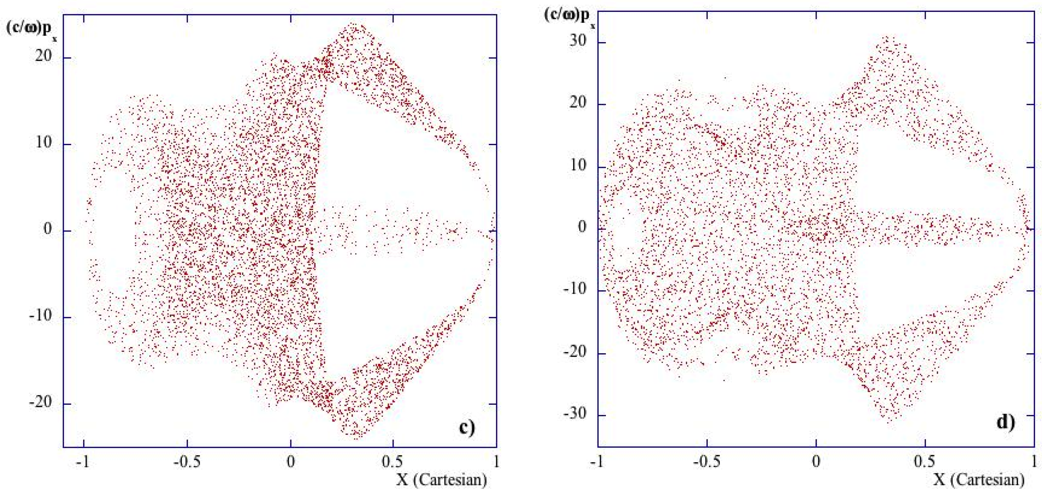
These articles we have mentioned provide important results on the existence or non-existence of an upper bound on the parallel wave number from an analytical study of the LH dispersion relation. 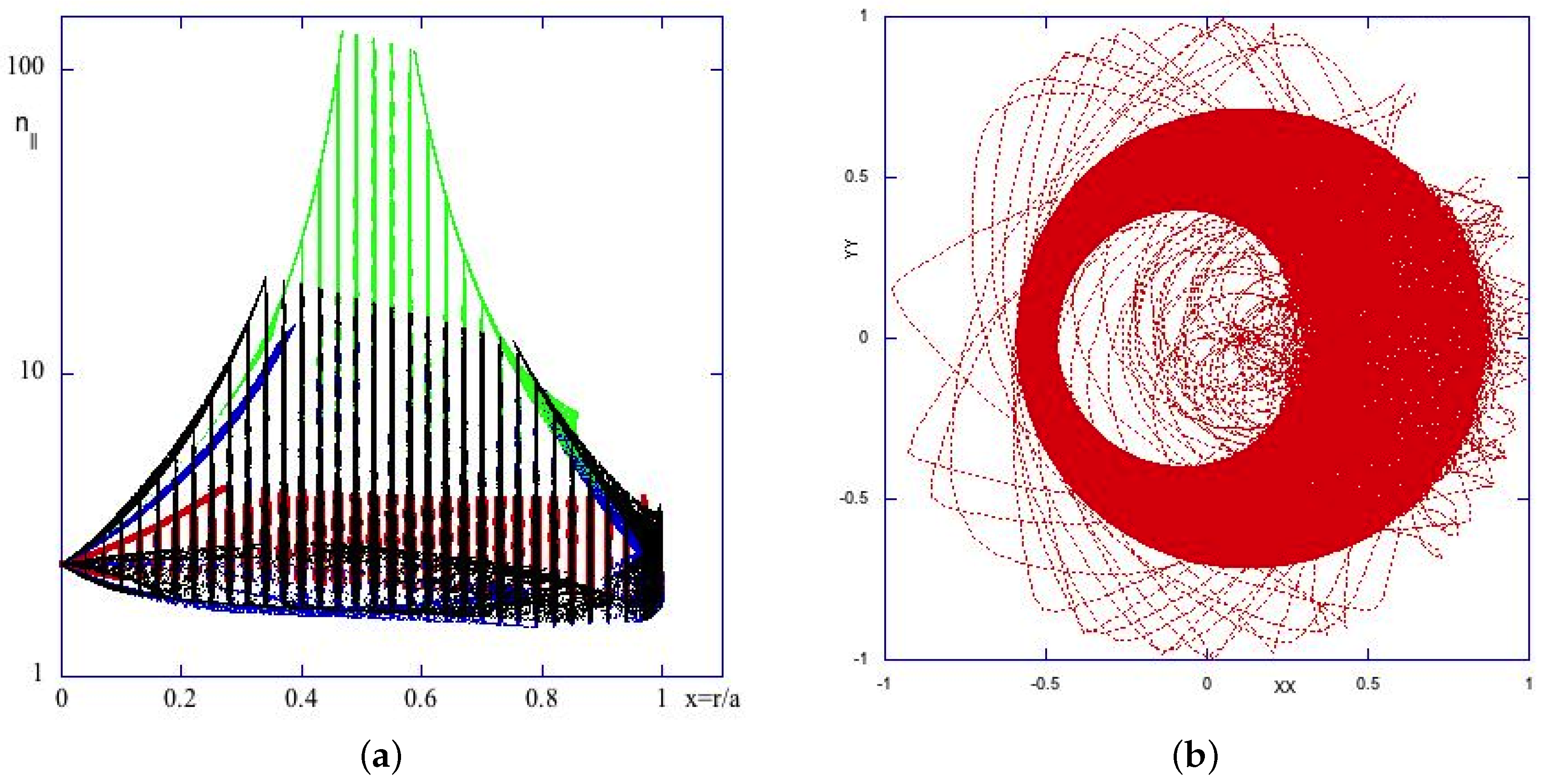From our study of the dynamics of the system, both from an analytical and a numerical point of view, we could deduce that the behavior of the system is regular for the experimentally-relevant range of plasma parameters, while it exhibits a chaotic behavior, with $n_{\parallel }$ experiencing a large increase, only if the central density $n_{e0}$ is high enough (that is, too high for usual LHCD experiments), which is in agreement with the conclusions of the cited articles. We also found, by a meticulous scan of the density parameter, that the plasma, for high values of the central density, enters a regime where the parallel wave number grows without limits. This singular behavior is shown in Figure 8a, where the range of $n_{\parallel }$, corresponding to increasingly higher central densities, is represented by the red, blue, green and black curves (corresponding respectively to the densities $3\times {10}^{13}{\text{cm}}^{-3}$, $9\times {10}^{13}{\text{cm}}^{-3}$, $1.2\times {10}^{14}{\text{cm}}^{-3}$ and $1.5\times {10}^{14}{\text{cm}}^{-3}$). The vertical bars correspond to the range of values of $n_{\parallel }$ for each different radial position, while the lateral continuous lines represent the upper bounds to the $n_{\parallel }$ upshifting. In particular, in the density range between $9\times {10}^{13}{\text{cm}}^{-3}$ and $1.2\times {10}^{14}{\text{cm}}^{-3}$, $n_{\parallel }$ reaches values higher than ${10}^2$, meaning that the oblique resonance mentioned above may be located somewhere in between. This picture has to be compared to the several plots shown in the papers quoted above, in particular with those from [50,51]. In Figure 8b, we show the trapping of the ray trajectories in the narrow region located at half-radius, where the phenomenon of wave number amplification occurs. The trapping of the trajectories is visible as an annular region in the poloidal section of the tokamak where the lines, corresponding to the ray trajectories, overlap and thicken considerably. This seems to agree with the presence of an attractor in the ray dynamics [53], which causes the ray trajectories to converge to a particular value of x, with increasingly smaller radial oscillations and larger values of $n_{\parallel }$. This last fact is compatible with the Hamiltonian nature of the system, because the phase-space volume of the system must be conserved.

It is worth noting that this phenomenon of the trapping of the trajectory in some zone in the phase-space that we have observed is very close to that analyzed by Zaslavsky in [54]. Without entering into the detail of the Zaslavsky analysis, we can says that the author describes three types of dynamical traps in Hamiltonian systems, which are due to the fact that trajectories stay close to some specific domains in phase space. Following the author, the dynamical trap is a domain in phase space where a particle (or its trajectory) can spend arbitrarily long finite time, performing almost regular dynamics, despite the fact that the full trajectory is random in any appropriate sense. It seems that our trajectory shown in Figure 8 is entering in a sub-domain of the phase space and remains trapped there for a long time. The symplectic nature of the Hamiltonian flow is in any case preserved, and the quenching of the trajectory in the physical space (Figure 8b) is accompanied by a large increase of the poloidal wavenumber and consequently of the parallel one.

9. Symplectic Algorithm

The numerical results obtained in Section 7 have been obtained using a second-order implicit symplectic algorithm [34], reported in Appendix B. We also performed a few simulations, over a time period corresponding to approximately 400 radial reflections of the rays, with both the symplectic algorithm and a fourth-order Runge–Kutta integrator. The simulations show that the curves corresponding to the time evolution of the variables overlap almost perfectly (Figure 9). A further check of the accuracy of the algorithm is provided by the conservation of energy. We computed the time evolution of energy in the simulations with the two algorithms. We see in Figure 10 that, in the Runge–Kutta integration, the energy slowly increases almost linearly with time, with a rate that is proportional to the time step used. This gradual increase would cause the simulation to become inaccurate if performed on a long time interval. On the contrary, in the symplectic integration, the energy oscillates around the initial value (that is zero) with an amplitude that is proportional to the time step used. This means that, on average, energy is conserved even for simulations performed over long time intervals (Figure 11). Early attempts to develop accurate symplectic integrators have been made by Ruth [55]; here, a third order symplectic algorithm was developed, which had the advantage of being explicit, but could be only applied to separable Hamiltonians. An improved version of this algorithm was developed by Candy and Rozmus [56]. Channel and Scovel [34] generalized the approach to non-separable Hamiltonians and developed an implicit symplectic algorithm, which can be implemented to arbitrary order of accuracy. In their paper, the authors show the superiority of their symplectic algorithm in comparison with a Runge–Kutta integrator for several different Hamiltonians. In particular, Figure 1 of [34] is analogous to our Figure 10. More recently, several different algorithms have been developed for general applications [35,36], and in particular, they have been applied to plasma-physics-related problems (see [37]). For our purposes, we chose a second order implicit symplectic algorithm inspired by Channel and Scovel. The results of our simulations, performed with both a fourth order Runge–Kutta integrator and the symplectic algorithm, show that the accuracy of the Runge–Kutta is high, even for integration times corresponding to hundreds of radial reflections of the wave. However, the energy is not conserved, and so, this could bring error accumulation on even longer times, with the consequent loss of accuracy in the simulation.

10. Conclusions

In this paper, we studied the LHW propagation in tokamaks by means of the Hamiltonian theory, by identifying the dispersion relation of the LH with a Hamiltonian. This is possible due to the axisymmetry, which characterizes the device and the use of the WKB approximation. The LH wave equation, to first order in the WKB expansion, can be seen as a Hamilton–Jacobi equation for the function S, which describes the surfaces of constant phase. The solution of this equation by the method of characteristics brings the Hamilton equations for the position $\overrightarrow{r}$ and the wave vector $\overrightarrow{k}$. In fact, the axisymmetry of the device results in the conservation of the toroidal component of the wave vector, which brings the equivalence between the characteristics equations and the Hamilton equations. We showed that the dispersion relation for the decoupled slow and fast wave branches in cylindrical geometry is analogous to the Hamiltonian of a 3D isotropic harmonic oscillator, and it is integrable. We were able to find the transformation from the original variables to the action-angle variables for this system, and we computed the ratio of the unperturbed frequencies of the radial and poloidal motion. The analytic calculations are made possible by the choice of a parabolic profile for the density, but the qualitative conclusions remain valid for an arbitrary choice of the radial density profile. When we pass to toroidal coordinates, the system changes from one dof to two dof, and the Hamiltonian is no longer integrable. Using the small inverse aspect-ratio ϵ, we were able to write the Hamiltonian as an integrable part plus a small perturbation, and we studied the effect of this two-dof perturbation on the unperturbed system by using the canonical perturbation theory. Keeping only the major terms in the perturbation, we saw that it cannot give rise to resonances between the frequencies of the unperturbed system, so the chaotic behavior of the dynamics seems to be excluded.

We performed numerical integrations of the ray equations to study the time evolution of the variables characterizing the system. The results show that the phase portrait of the radial coordinate and the corresponding wave number is not closed, due to the non-integrability of the system, but the trajectory remains bounded without covering the entire phase space, even for long integration times, at least in the range of parameters typical of real experiments. The calculation of the parallel wave number shows that its value varies in time due to the non-conservation of the poloidal wave number, but in the range of parameters typical of the LHCD experiments on FTU, its time-average remains limited to low values, so that it cannot give rise to significant absorption by Landau damping. We observed instead a different behavior in the dynamics of the system depending on the value of the central density $n_{e0}$. In the lower density case $n_{e0}=5\times {10}^{13}{\text{cm}}^{-3}$, we found that the system behaves regularly, with ray trajectories, which do not fill completely the “energetically” available phase space portion, a very regular Poincaré section and a small increase in the time-averaged $n_{\parallel }$. In the higher density case $n_{e0}={10}^{14}{\text{cm}}^{-3}$, the system shows a chaotic behavior, with ray trajectories that fill almost completely the “energetically” available phase space portion, an irregular Poincaré section and a large increase in the time-averaged $n_{\parallel }$. Since the central density enters the “energy” of the system in the slow and fast branches through the plasma frequency ${\omega }_{pe0}^2$ (see Equations (14)–(16)), we can deduce that the behavior of the system remains regular as long as its “energy” is low enough. We also observed a weak dependence on the value of the safety factor at the edge $q_a$, which can be again ascribed to the dependence of the “energy” of the system on the safety factor. However, the irregular behavior only appears in the unrealistic high central density case, which is not typical of LHCD experiments. By performing a more accurate scan of the parameters, we found that a singular behavior occurs in a very narrow range of central densities, where the value of $n_{\parallel }$ seems to increase without limit and the ray trajectories remain trapped in a narrow intermediate region. This effect can be attributed to the presence of an oblique resonance [52], where both $n_{\perp }$ and $n_{\parallel }$ go to infinity, their ratio remaining finite. The increase of $n_{\perp }$ and $n_{\parallel }$ comes with a trapping of the ray trajectories in a narrow intermediate radial region of the plasma volume, due to the presence of an attractor for the orbits of the system. This effect was predicted theoretically [52,53], but to our knowledge, its importance has never been fully recognized.