Second Law Analysis of Adiabatic and Non-Adiabatic Pipeline Flows of Unstable and Surfactant-Stabilized Emulsions

Abstract

Entropy generation, and hence exergy destruction, in adiabatic flow of unstable and surfactant-stabilized emulsions was investigated experimentally in different diameter pipes. Four types of emulsion systems are investigated covering a broad range of the dispersed-phase concentration: (a) unstable oil-in-water (O/W) emulsions without surfactant; (b) surfactant-stabilized O/W emulsions; (c) unstable water-in-oil (W/O) emulsions without surfactant; and (d) surfactant-stabilized W/O emulsions. The entropy generation rate per unit pipe length is affected by the type of the emulsion as well as its stability. Unstable emulsions without any surfactant present at the interface generate less entropy in the turbulent regime as compared with the surfactant-stabilized emulsions of the same viscosity and density. The effect of surfactant is particularly severe in the case of W/O emulsions. In the turbulent regime, the rate of entropy generation in unstable W/O emulsions is much lower in comparison with that observed in the stable W/O emulsions. A significant delay in the transition from laminar to turbulent regime is also observed in the case of unstable W/O emulsion. Finally, the analysis and simulation results are presented on non-adiabatic pipeline flow of emulsions.

1. Introduction

A significant portion of the electrical energy produced in the world is consumed by pumping systems [1]. In some industrial applications, nearly 50% of the total electrical energy used in the process is consumed by the the pumps alone [1]. Thus it is of practical importance to carry out a second law analysis of a pumping system to determine the extent to which energy is dissipated due to irreversibilities in the process.

The amount of work lost due to irreversibilities in the process is related to the total exergy destruction and total entropy generation in the process [2,3,4,5] as follows:

$${\dot{W}}_{lost}={\dot{\mathsf{\Psi }}}_{D,total}=T_o{\dot{S}}_{G,total}$$

(1)

where ${\dot{W}}_{lost}$ is the rate of lost work and ${\dot{\mathsf{\Psi }}}_{D,total}$ is the total rate of exergy destruction in the process, including both the internal destruction within the control volume and the external destruction outside the control volume, $T_o$ is the temperature of the surroundings, and ${\dot{S}}_{G,total}$ is the total rate of entropy generation. Equation (1) is the Gouy-Stodola theorem [5] which states that the total rate of exergy destruction in the process is linearly proportional to the total rate of entropy production in the system and the surroundings. The higher the rate of exergy destruction, the higher is the amount of energy that becomes unavailable for work. Note that the thermo-mechanical exergy associated with a fluid stream per unit mass is defined as follows:

$$\mathsf{\psi }=\left(h-h_o\right)-T_o\left(s-s_o\right)+\frac{V^2}{2}+gz$$

(2)

where $h$ and $s$ are specific enthalpy and specific entropy of fluid, respectively, $h_o$ and $s_o$ are specific enthalpy and specific entropy of fluid in the dead state, respectively, $V$ is the fluid velocity, $g$ is the acceleration due to gravity, and $z$ is the elevation of the fluid stream with respect to the dead state.

This article is related to entropy production, and hence exergy destruction, in pipeline flow of unstable and surfactant-stabilized emulsions. Emulsions are two-phase dispersions of oil and water. They are utilized in a variety of engineering applications and systems [6,7,8,9,10,11,12]. Emulsions can be classified as either oil-in-water (abbreviated as O/W) type or water-in-oil (abbreviated as W/O) type. In O/W emulsions, oil droplets are dispersed in a continuum of water phase and in W/O emulsions, water droplets are dispersed in a continuum of oil phase. Thus W/O emulsions are inverse of O/W emulsions structurally. Both types of emulsions are important industrially [6]. In a number of applications, the emulsions are transported from one location to another by pumping them through the pipelines. As these pumping systems consume a significant amount of total electrical energy used in the process, it is important to be able to quantify the amount of energy dissipation or work lost in terms of entropy generation and exergy destruction.

A number of papers have been published on pipeline flow of emulsions in the past [8,9,10]. However, these publications are restricted to pressure losses in adiabatic flows. The interpretation and analysis of adiabatic and non-adiabatic pipeline flows of emulsions in terms of exergy destruction and entropy generation and the second law of thermodynamics are lacking. The second law analysis of a process is important from a practical point of view. The key advantage of the second law analysis of a process is that it allows comparisons of irreversible effects resulting from different mechanisms in the same process. For example, in non-adiabatic flows entropy generation occurs due to irreversible heat transfer as well as due to fluid friction. The comparisons of entropy generation rates due to different mechanisms is important for the design engineer to identify the dominant mechanism of exergy destruction in the process.

This work is in continuation of our earlier studies on the production of entropy and destruction of exergy in pipeline flow of emulsions [13,14,15]. Our earlier studies were restricted to only adiabatic flows of emulsions in pipes. Furthermore, the experimental data involved only a single type of emulsions. In this study, we consider four different types of emulsion systems together: (a) unstable oil-in-water (O/W) emulsions without surfactant; (b) surfactant-stabilized O/W emulsions; (c) unstable water-in-oil (W/O) emulsions without surfactant; and (d) surfactant-stabilized W/O emulsions. The experimental data obtained for different emulsion systems are compared and conclusions are drawn on the influence of stability and type of emulsions on entropy generation and exergy destruction in adiabatic pipeline flow of emulsions. The second law analysis and simulation results dealing with non-adiabatic flow of emulsions in pipelines are also presented.

2. Theoretical Background

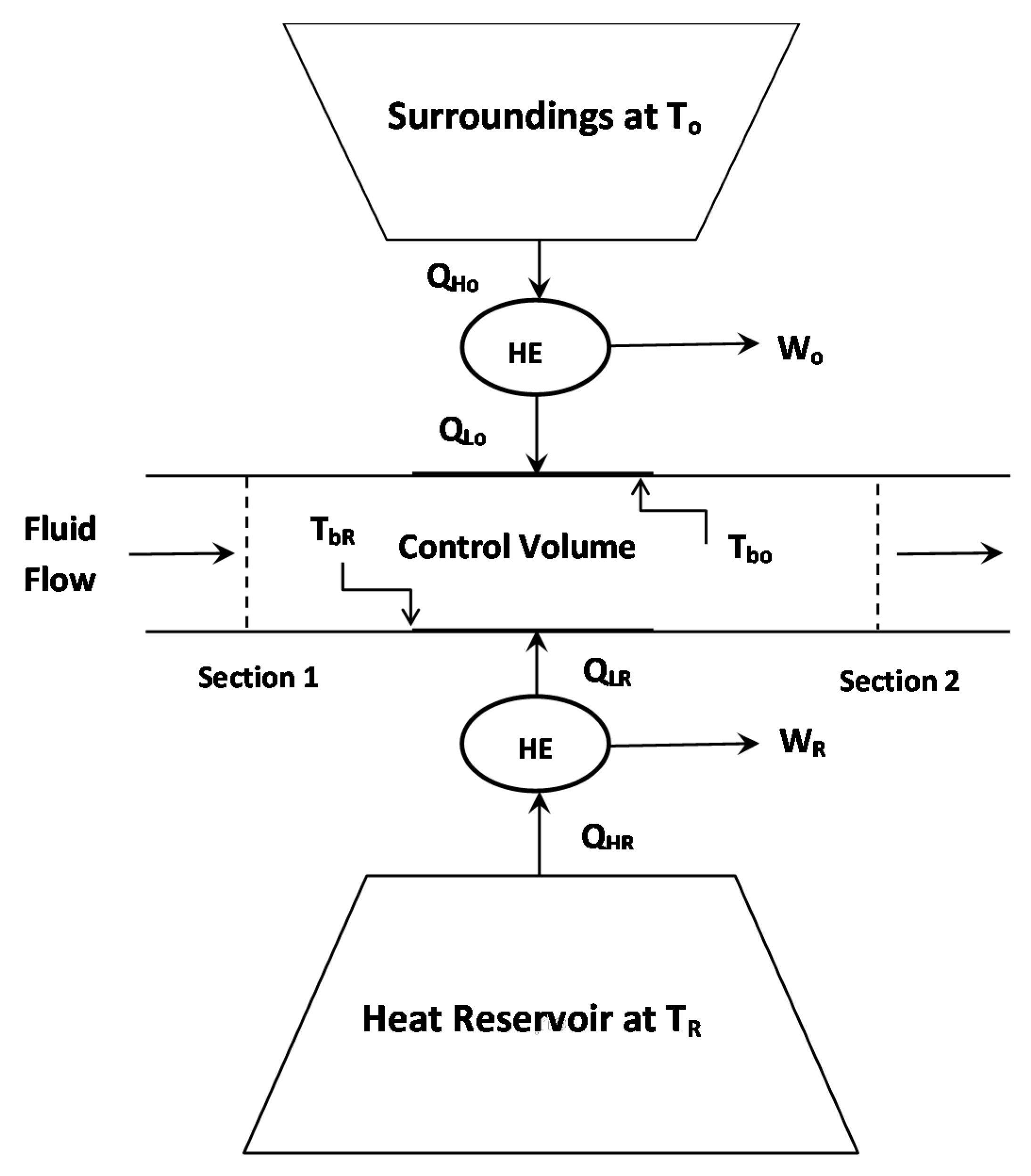
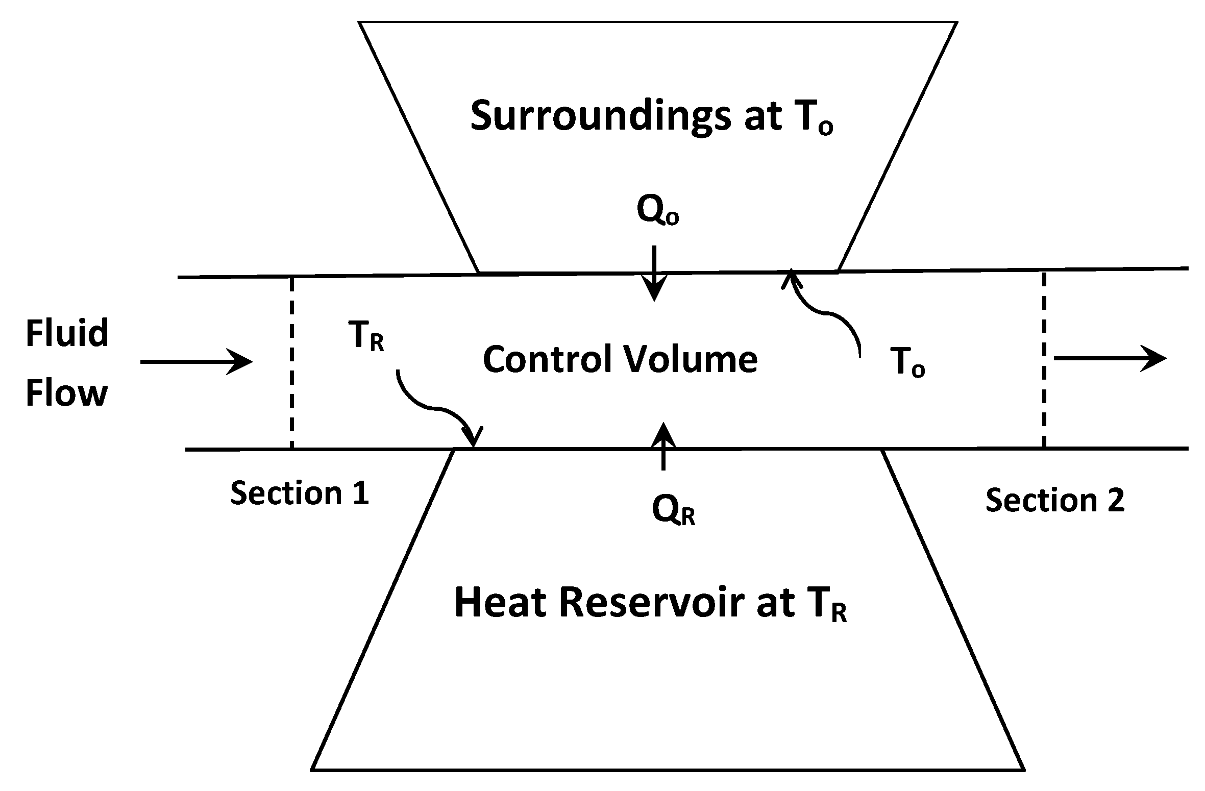
2.1. Non-Adiabatic Flow

Consider non-adiabatic flow of fluid in a pipe, as shown in Figure 1. The fluid is receiving heat from both the surroundings (which constitute a heat reservoir at constant temperature $T_o$) and a heat reservoir at constant temperature $T_R$. Let the rate of heat transfer from the surroundings at $T_o$ to the control volume be ${\dot{Q}}_o$ and the rate of heat transfer from the heat reservoir at $T_R$ to the control volume be ${\dot{Q}}_R$. There is no shaft work being produced from the control volume. Let $\mathsf{\psi }$ be the exergy of fluid per unit mass and $\mathsf{\Psi }$ be the total exergy. Let the temperatures at the control volume boundary portions in contact with the surroundings and the heat reservoir be $T_{bo}$ and $T_{bR}$, respectively. Exergy balance on the control volume gives:

$${\dot{m}}_1{\mathsf{\psi }}_1+{\dot{Q}}_o\left[1-\frac{T_o}{T_{bo}}\right]+{\dot{Q}}_R\left[1-\frac{T_o}{T_{bR}}\right]-{\dot{m}}_2{\mathsf{\psi }}_2-{\dot{\mathsf{\Psi }}}_{D,CV}=\frac{\partial {\mathsf{\Psi }}_{CV}}{\partial t}$$

(3)

where $\dot{m}$ is mass flow rate, subscript “$1$” refers to inlet, subscript “$2$” refers to outlet, subscript “$CV$” refers to control volume, and ${\dot{\mathsf{\Psi }}}_{D,CV}$ is the rate of exergy destruction in the control volume. Thus:

$${\dot{\mathsf{\Psi }}}_{D,CV}={\dot{m}}_1{\mathsf{\psi }}_1+{\dot{Q}}_o\left[1-\frac{T_o}{T_{bo}}\right]+{\dot{Q}}_R\left[1-\frac{T_o}{T_{bR}}\right]-{\dot{m}}_2{\mathsf{\psi }}_2-\frac{\partial {\mathsf{\Psi }}_{CV}}{\partial t}$$

(4)

Only when the process is internally-reversible, ${\dot{\mathsf{\Psi }}}_{D,CV}=0$. For an internally-irreversible process, ${\dot{\mathsf{\Psi }}}_{D,CV}>0$. Doing exergy balance on the surroundings including the heat reservoir at $T_R$, one can write:

$$-{\dot{Q}}_o\left[1-\frac{T_o}{T_{bo}}\right]-{\dot{Q}}_R\left[1-\frac{T_o}{T_{bR}}\right]-{\dot{\mathsf{\Psi }}}_{D,surr}=\frac{\partial {\mathsf{\Psi }}_{surr}}{\partial t}=-{\dot{Q}}_R\left[1-\frac{T_o}{T_R}\right]$$

(5)

where ${\dot{\mathsf{\Psi }}}_{D,surr}$ is the rate of exergy destruction in the surroundings (including the heat reservoir at $T_R$). This equation could be re-cast as:

$${\dot{\mathsf{\Psi }}}_{D,surr}=T_o\left[\frac{{\dot{Q}}_o}{T_{bo}}\left(1-\frac{T_{bo}}{T_o}\right)+\frac{{\dot{Q}}_R}{T_{bR}}\left(1-\frac{T_{bR}}{T_R}\right)\right]$$

(6)

Note that each term on the right-hand side of this equation is positive, that is, ${\dot{\mathsf{\Psi }}}_{D,surr}>0$. Only when heat is transferred reversibly to the control volume, ${\dot{\mathsf{\Psi }}}_{D,surr}=0$. In principle, the heat could be transferred reversibly to the control volume either by placing the heat reservoirs directly at the control volume boundary, as shown in Figure 2, such that $T_{boundary}=T_{heat-reservoir}$, or by installing Carnot heat engines between the control volume boundary and heat reservoirs, as shown in Figure 3. For the scheme shown in Figure 2, the exergy balance on the surroundings gives:

$$-{\dot{Q}}_R\left[1-\frac{T_o}{T_R}\right]-{\dot{\mathsf{\Psi }}}_{D,surr}=\frac{\partial {\mathsf{\Psi }}_{surr}}{\partial t}$$

(7)

where:

$$\frac{\partial {\mathsf{\Psi }}_{surr}}{\partial t}=-{\dot{Q}}_R\left[1-\frac{T_o}{T_R}\right]$$

(8)

Combining Equations (7) and (8) gives ${\dot{\mathsf{\Psi }}}_{D,surr}=0$, as expected in the absence of external irreversibilities. For the scheme shown in Figure 3, the exergy balance on the surroundings gives:

$$-{\dot{Q}}_{Lo}\left[1-\frac{T_o}{T_{bo}}\right]-{\dot{Q}}_{LR}\left[1-\frac{T_o}{T_{bR}}\right]-{\dot{\mathsf{\Psi }}}_{D,surr}=\frac{\partial {\mathsf{\Psi }}_{surr}}{\partial t}$$

(9)

where:

$$\frac{\partial {\mathsf{\Psi }}_{surr}}{\partial t}={\dot{W}}_o+{\dot{W}}_R-{\dot{Q}}_{HR}\left[1-\frac{T_o}{T_R}\right]$$

(10)

Combining Equations (9) and (10) gives:

$${\dot{\mathsf{\Psi }}}_{D,surr}=-{\dot{Q}}_{Lo}\left[1-\frac{T_o}{T_{bo}}\right]-{\dot{Q}}_{LR}\left[1-\frac{T_o}{T_{bR}}\right]-\left[{\dot{W}}_o+{\dot{W}}_R-{\dot{Q}}_{HR}\left(1-\frac{T_o}{T_R}\right)\right]$$

(11)

Using the following relations: ${\dot{Q}}_{L0}/T_{bo}={\dot{Q}}_{H0}/T_o$, ${\dot{Q}}_{LR}/T_{bR}={\dot{Q}}_{HR}/T_R$, ${\dot{W}}_o={\dot{Q}}_{Ho}-{\dot{Q}}_{Lo}$, and ${\dot{W}}_R={\dot{Q}}_{HR}-{\dot{Q}}_{LR}$, Equation (11) reduces to ${\dot{\mathsf{\Psi }}}_{D,surr}=0$ as expected in the absence of external irreversibilities.

For the actual process shown in Figure 1 where both internal and external irreversibilities are present, the total rate of exergy destruction can be obtained by adding the exergy balances for $CV$ (Equation (4)) and surroundings (Equation (6)):

$${\dot{\mathsf{\Psi }}}_{D,total}={\dot{\mathsf{\Psi }}}_{D,CV}+{\dot{\mathsf{\Psi }}}_{D,surr}={\dot{m}}_1{\mathsf{\psi }}_1-{\dot{m}}_2{\mathsf{\psi }}_2+{\dot{Q}}_R\left[1-\frac{T_o}{T_R}\right]-\frac{\partial {\mathsf{\Psi }}_{CV}}{\partial t}$$

(12)

From the second law of thermodynamics:

$${\dot{\mathsf{\Psi }}}_{D,total}=\left[{\dot{m}}_1{\mathsf{\psi }}_1-{\dot{m}}_2{\mathsf{\psi }}_2\right]+{\dot{Q}}_R\left[1-\frac{T_o}{T_R}\right]+\left[-\frac{\partial {\mathsf{\Psi }}_{CV}}{\partial t}\right]\ge 0$$

(13)

Note that the first square-bracketed term on the right hand side of Equation (13) is simply the net rate of decrease of exergy of the flowing stream, the second term is the rate of decrease of exergy of the surroundings, and the third term is the rate of decrease of exergy of the fluid contained within the control volume. Thus, the work lost in the process under steady state conditions can be expressed as:

$${\dot{W}}_{lost}={\dot{\mathsf{\Psi }}}_{D,total}=\dot{m}\left({\mathsf{\psi }}_1-{\mathsf{\psi }}_2\right)+{\dot{Q}}_R\left[1-\frac{T_o}{T_R}\right]\ge 0$$

(14)

2.2. Adiabatic Flow

Consider now the steady and adiabatic flow of fluid in a pipe without any shaft work. According to Equation (14):

$${\dot{W}}_{lost}={\dot{\mathsf{\Psi }}}_{D,total}=\dot{m}\left({\mathsf{\psi }}_1-{\mathsf{\psi }}_2\right)=\dot{m}\left[\left(\left(h_1-h_2\right)-T_o\left(s_1-s_2\right)+\left(\frac{V_1^2}{2}-\frac{V_2^2}{2}\right)+\left(z_1-z_2\right)g\right)\right]$$

(15)

Neglecting kinetic and potential energy changes, Equation (15) reduces to:

$${\dot{W}}_{lost}={\dot{\mathsf{\Psi }}}_{D,total}=\dot{m}\left[T_o\mathsf{\Delta }s-\mathsf{\Delta }h\right]$$

(16)

As $\mathsf{\Delta }h=0$ for adiabatic incompressible flow without shaft work and with negligible kinetic and potential energy changes, Equation (16) becomes:

$${\dot{W}}_{lost}={\dot{\mathsf{\Psi }}}_{D,total}=\dot{m}\left(T_o\mathsf{\Delta }s\right)$$

(17)

This equation could be re-written in terms of the total rate of entropy production ${\dot{S}}_{G,total}$ by noting that in the present case of adiabatic flow, entropy is generated only within the control volume:

$${\dot{S}}_{G,total}={\dot{S}}_{G,CV}=\dot{m}\mathsf{\Delta }s$$

(18)

Thus:

$${\dot{W}}_{lost}={\dot{\mathsf{\Psi }}}_{D,total}=T_o{\dot{S}}_{G,total}$$

(19)

Equation (19) is the same as Equation (1), the well-known Gouy-Stodola theorem [5,16].

Entropy Production in Adiabatic Pipeline Flow

It can be readily shown that ${\dot{S}}_G^{\prime }$, the rate of entropy generation per unit length of pipe, in incompressible adiabatic flow is given as [13,15]:

$${\dot{S}}_G^{\prime }=\dot{m}\frac{ds}{dx}=\frac{\dot{m}}{\mathsf{\rho }T}\left(-\frac{dP}{dx}\right)$$

(20)

where T is the fluid temperature, $\mathsf{\rho }$ is the density, and dP/dx is the pressure gradient in the direction of flow. Assuming the fluid to be Newtonian of constant density and viscosity, Equation (20) could be re-cast in terms of the friction factor and Reynolds number as [13,15]:

$${\dot{S}}_G^{\prime }=\frac{\mathsf{\pi }}{2T}\left(\frac{{\mathsf{\mu }}^3}{{\mathsf{\rho }}^2{D}^2}\right)\left(f{\mathrm{Re}}^3\right)$$

(21)

where D is the pipe diameter, μ is the fluid viscosity, f is the Fanning friction factor, Re is the pipe Reynolds number defined as $\mathsf{\rho }D\overline{V}/\mathsf{\mu }$, and $\overline{V}$ is the average fluid velocity in pipe.

For laminar hydrodynamically fully developed flow of incompressible Newtonian fluids in pipes, the Fanning friction factor is related to the Reynolds number as follows:

$$f=\frac{16}{\mathrm{Re}}$$

(22)

The friction factor is independent of the pipe roughness in laminar regime. For hydrodynamically fully developed turbulent flow of incompressible Newtonian fluids in pipes, the friction factor is given by the following Blasius equation:

$$f=\frac{0.079}{{\mathrm{Re}}^{1/4}}$$

(23)

The Blasius equation gives good predictions of friction factor in the Re range of 3000 to 100,000. Note that the Blasius equation does not account for the pipe roughness. In turbulent flows, the friction factor increases with the increase in pipe roughness. Thus the Blasius equation is restricted to turbulent flows in hydraulically-smooth pipes. Upon substitution of the friction factor expressions from Equations (22) and (23) into Equation (21), the following relations are obtained for entropy generation in pipeline flows:

$${\dot{S}}_G^{\prime }=\frac{\mathsf{\pi }}{2T}\left(\frac{{\mathsf{\mu }}^3}{{\mathsf{\rho }}^2{D}^2}\right)\left(16{\mathrm{Re}}^2\right)$$

(24)

$${\dot{S}}_G^{\prime }=\frac{\mathsf{\pi }}{2T}\left(\frac{{\mathsf{\mu }}^3}{{\mathsf{\rho }}^2{D}^2}\right)\left(0.079{\mathrm{Re}}^{2.75}\right)$$

(25)

Equation (24) is restricted to the laminar regime and Equation (25) is valid for turbulent flow of Newtonian fluids in hydraulically-smooth pipes. Equations (24) and (25) could be used to predict entropy generation per unit length in pipeline flow of pseudo-homogeneous mixtures of two phases such as emulsions of oil and water provided that the mixtures are Newtonian in nature.

3. Experimental Work: Adiabatic Pipeline Flow of Emulsions

The entropy generation rates in adiabatic pipeline flow of unstable and surfactant-stabilized W/O and O/W emulsions were investigated experimentally in two different diameter pipes. The pipes were hydraulically smooth (stainless steel, seamless) and were installed horizontally. The dimensions of the pipeline test sections are summarized in

Table 1. Dimensions of pipeline flow test sections.

Pipe Inside Diameter (mm)	Entrance Length (m)	Length of Test Section (m)	Exit Length (m)
8.89	0.89	3.35	0.48
15.8	1.65	2.59	0.56

.

The emulsions were prepared in a large mixing tank (capacity about 1 m³) at room temperature (25 °C). The tank was equipped with baffles, high shear impeller-type mixers, heating/cooling coil, and a temperature controller. The emulsion prepared in the mixing tank was circulated to the pipeline test sections, one at a time, by a centrifugal pump. The pressure drops in the pipeline test sections were measured by means of the pressure transducers. The flow rate of the emulsion was measured by allowing it to pass through the metering section equipped with electro-magnetic and orifice flowmeters before returning to the mixing tank. For each pipeline test section, enough entry length (more than 100 pipe diameters) was provided for the flow to become hydrodynamically fully developed. The exit lengths after the test sections were in the range of 35 to 55 pipe diameters. The pressure transducers and the flow meters were all calibrated prior to any experimental work. The friction factor versus Reynolds number data obtained from the pipeline test sections using single-phase Newtonian fluids were found to be in good agreement with the standard friction factor relations valid for the laminar and turbulent flow of single-phase Newtonian fluids. Further details about the experimental set-up can be found in our earlier publications [13,14,15].

Four sets of emulsions (unstable O/W, surfactant-stabilized O/W, unstable W/O, and surfactant-stabilized W/O) were prepared. The composition and the type of emulsions prepared in this work are given in

Table 2. Information about the emulsions prepared in the present work.

Emulsion-Type	Oil-Phase	Aqueous-Phase	Dispersed-Phase Concentrations (% Vol.)
Unstable O/W (Set 1)	Refined mineral oil (Bayol-35)	Tap water	28.76; 44.98; 55.07
Surfactant-stabilized O/W (Set 2)	Refined mineral oil (Bayol-35)	1% by wt. surfactant solution in tap water; the surfactant used was Triton X-100 (isooctylphenoxypolyethoxy ethanol)	16.53; 30.4; 44.41; 49.65; 55.14
Unstable W/O (Set 3)	Refined mineral oil (Bayol-35)	Tap water	0; 10.51; 17.49; 26.72; 32.47; 38.14; 41.05
Surfactant-stabilized W/O (Set 4)	1.5% by wt. surfactant solution in mineral oil (Bayol-35); the surfactant used was SPAN-80 (sorbitan monooleate)	Tap water	0; 10.61; 18.25; 25.85

. A refined mineral oil (Bayol-35) and tap water were used to prepare the emulsions. The density of the oil was 780 kg/m³ and its viscosity was 2.41 mPa·s at 25 °C. The experiments were started with continuous phase (oil, oil-surfactant mixture, water, water-surfactant mixture, depending on the type of emulsion) into which a required amount of the dispersed-phase was added to prepare an emulsion. The concentration of the dispersed-phase was increased by successive additions of the dispersed-phase. The temperature of the emulsion was maintained constant at 25 °C with the help of a temperature controller installed in the mixing tank.

Measurement Uncertainties

The uncertainties in the measurement of the various quantities at 95% confidence level were as follows: volumetric flow rate—less than 1%, length of test section—less than 0.5%, diameter of pipe—less than 0.3%, density of fluid—less than 1%, viscosity of fluid—less than 1.5%, and pressure drop—less than 1%. According to the standard error analysis using the propagation of errors, the uncertainty in the reported friction factor is less than 3% and the uncertainty in the reported Reynolds number is less than 2.1%. The uncertainty in the measurement of the dispersed-phase concentration was less than 2%.

4. Results and Discussion: Adiabatic Pipeline Flow of Emulsions

In analyzing the experimental measurements, it is assumed that emulsions can be treated as pseudo-homogeneous mixtures with average properties. Strictly speaking, emulsions are heterogeneous systems consisting of discrete droplets of one phase suspended in a continuum of another phase. Nevertheless, they are widely treated as homogeneous fluids when it comes to defining their macroscopic flow behavior [6]. The treatment of emulsions as homogeneous fluids with average properties is justified as long as the length scale of the apparatus ($L$) is large in comparison with the average spacing ($\ell$) between the centers of the adjacent droplets [6]. When $L>>l$, a representative volume element of an emulsion of volume $V$ whose linear dimension, $V^{1/3}$, is small compared to $L$ but large compared to $\ell$ ($\ell$ << $V^{1/3}$ << $L$), is large enough to contain a statistically significant number of droplets so that one can define the bulk or average fields as volume averages of the corresponding local fields over the representative element. This volume averaging technique is a standard technique used extensively in the literature [6] in modeling the rheology of dispersed systems to define the bulk or average stress and rate of strain tensors. The condition $L>>l$ is readily met in the present work as emulsion droplets were very small in comparison with the pipe diameters. For example, the droplets were smaller than 5 µm in diameter in stable W/O emulsions and smaller than 10 µm in diameter in stable O/W emulsions . Thus the flow of emulsions in this work is treated as homogeneous flow with average properties. The additional restrictions are: the flow is steady and hydrodynamically fully-developed.

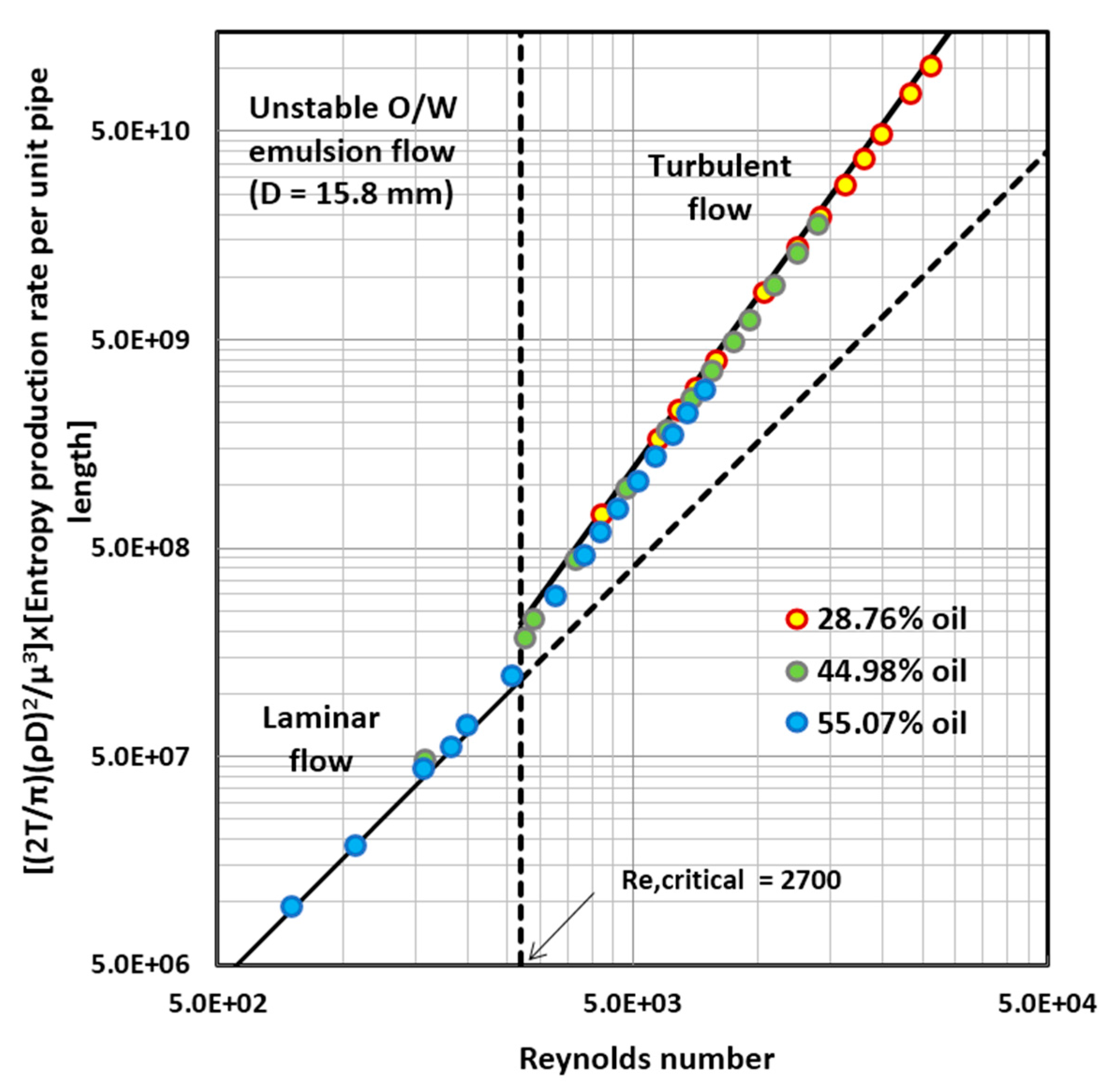
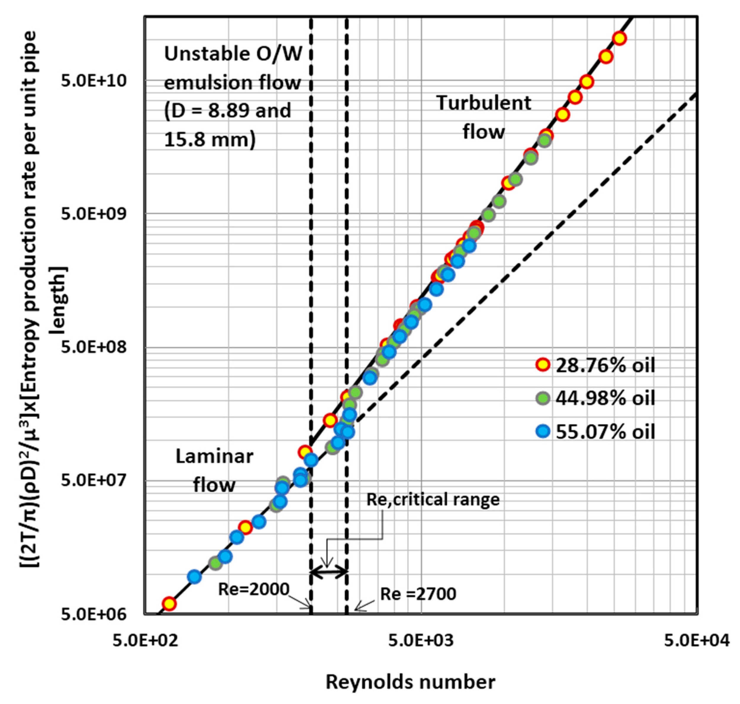
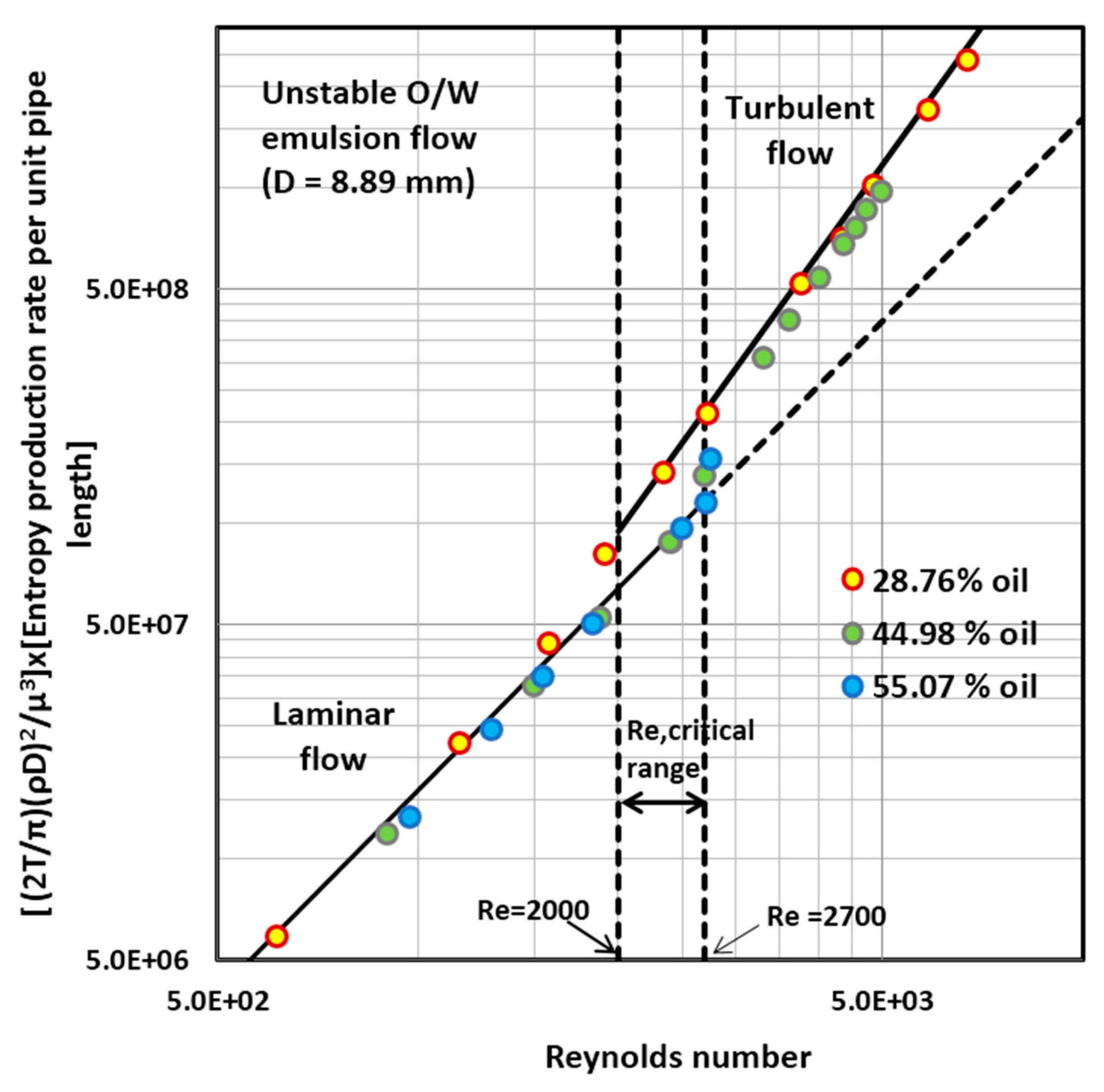
4.1. Entropy Generation in Adiabatic Pipeline Flow of Unstable Oil-in-Water (O/W) Emulsions

The rate of entropy generation per unit pipe length (${\dot{S}}_G^{\prime }$) can be determined from experimental measurements using Equation (21). It requires the knowledge of friction factor, fluid properties ($\mathsf{\mu }$ and $\mathsf{\rho }$), Reynolds number, pipe diameter, and fluid temperature ($T$). In the present study, $T=298.15\mathrm{K}$. The friction factor is obtained from the pressure-drop versus flow rate measurements using the following relation:

$$f=\frac{(-dP/dx)(D/4)}{\mathsf{\rho }{\overline{V}}^2/2}$$

(26)

where D is the pipe diameter and $\overline{V}$ is the average fluid velocity in pipe.

The experimental data are analyzed in terms of a dimensionless rate of entropy generation, defined as:

$${({\dot{S}}_G^{\prime })}^{\ast }=\frac{{\dot{S}}_G^{\prime }}{\frac{\mathsf{\pi }}{2T}\left(\frac{{\mathsf{\mu }}^3}{{\mathsf{\rho }}^2{D}^2}\right)}$$

(27)

According to Equations (24) and (25), the dimensionless rate of entropy generation ${({\dot{S}}_G^{\prime })}^{\ast }$ is a function of Reynolds number only. Thus the experimental data for differently-concentrated emulsions of different viscosities and densities from different diameter pipes should all fall on the same ${({\dot{S}}_G^{\prime })}^{\ast }$ versus Re line for a given flow regime (laminar or turbulent).

Figure 4 shows the plot of dimensionless rate of entropy generation ${({\dot{S}}_G^{\prime })}^{\ast }$ versus $\mathrm{Re}$ data for differently concentrated unstable O/W emulsions, without the presence of any surfactant. The data shown in Figure 4 were collected from 8.89 mm diameter pipe. The experimental data are compared with Equations (24) and (25), re-written in dimensionless form as:

$${({\dot{S}}_G^{\prime })}^{\ast }=\frac{{\dot{S}}_G^{\prime }}{\frac{\mathsf{\pi }}{2T}\left(\frac{{\mathsf{\mu }}^3}{{\mathsf{\rho }}^2{D}^2}\right)}=16{\mathrm{Re}}^2$$

(28)

$${({\dot{S}}_G^{\prime })}^{\ast }=\frac{{\dot{S}}_G^{\prime }}{\frac{\mathsf{\pi }}{2T}\left(\frac{{\mathsf{\mu }}^3}{{\mathsf{\rho }}^2{D}^2}\right)}=0.079{\mathrm{Re}}^{2.75}$$

(29)

In the laminar regime, the experimental data fall on the line representing Equation (28). However, the turbulent flow data fall somewhat below the prediction of Equation (29) indicating some degree of drag-reduction behavior on the part of unstable O/W emulsions. Furthermore, there occurs a significant delay in transition from laminar to turbulent regime, especially when the dispersed-phase (oil) concentration is high. For 28.76% by volume O/W emulsion, transition occurs at a Reynolds number of about 2000. For O/W emulsions with dispersed-phase concentrations of 44.98% and 55.07% by volume, the transition from laminar to turbulent flow occurs at a Reynolds number of about 2700.

Figure 5 shows ${({\dot{S}}_G^{\prime })}^{\ast }$ versus $\mathrm{Re}$ data for unstable O/W emulsions obtained from a larger diameter pipe (diameter of 15.8 mm). The experimental data from 15.8 mm diameter pipe confirm the observations that concentrated unstable O/W emulsions exhibit drag reduction to some degree in turbulent regime and that there occurs a delay in transition from laminar to turbulent regime.

Figure 6 shows all the experimental data obtained from two different diameter pipes for differently concentrated unstable O/W emulsions. The dimensionless rate of entropy generation data for emulsions fall on the same line for a given flow regime, as expected from Equations (28) and (29), regardless of the pipe diameter and viscosity and density of emulsion.

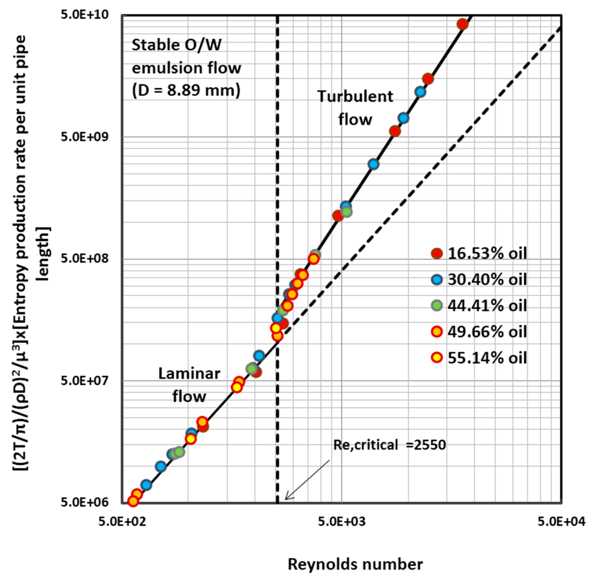
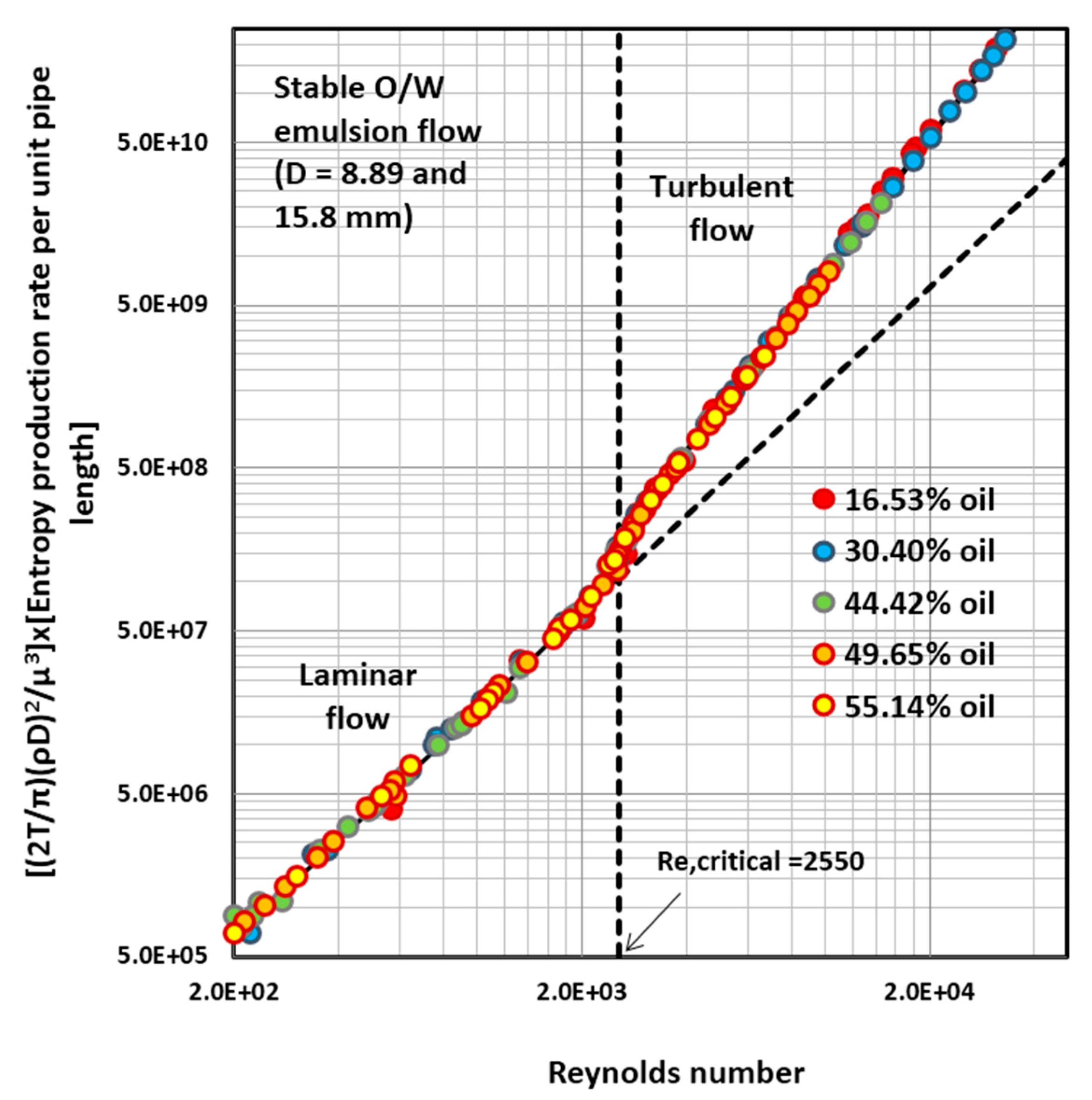
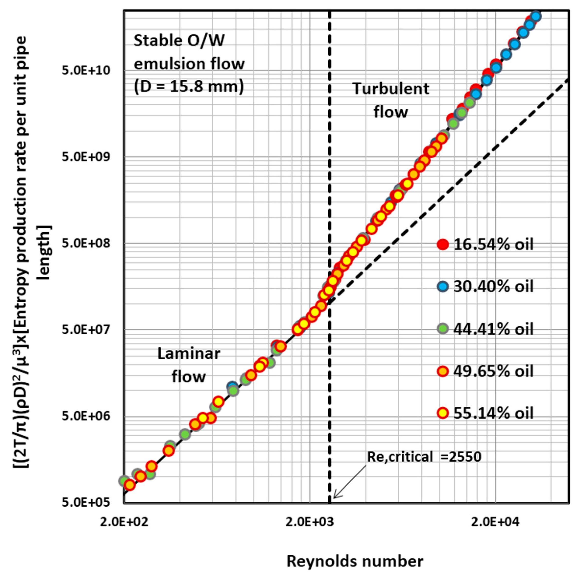
4.2. Entropy Generation in Adiabatic Pipeline Flow of Surfactant-Stabilized Oil-in-Water (O/W) Emulsions

Figure 7 shows the plot of dimensionless rate of entropy generation ${({\dot{S}}_G^{\prime })}^{\ast }$ versus $\mathrm{Re}$ data for differently concentrated surfactant-stabilized O/W emulsions. The data shown in Figure 7 were collected from 8.89 mm diameter pipe. Clearly the experimental data for surfactant-stabilized O/W emulsions follow the theoretical lines (Equation (28) for laminar regime and Equation (29) for turbulent regime). The transition from laminar to turbulent flow occurs at a Reynolds number of about 2550. The transition Reynolds number is somewhat higher than that expected for single-phase Newtonian fluids. Thus there occurs some delay in the transition from laminar to turbulent regime in the presence of surfactant-stabilized droplets.

Figure 8 shows ${({\dot{S}}_G^{\prime })}^{\ast }$ versus $\mathrm{Re}$ data for surfactant-stabilized O/W emulsions obtained from a larger diameter pipe (diameter of 15.8 mm). The experimental data from 15.8 mm diameter pipe are consistent with the observations that surfactant-stabilized O/W emulsions do not exhibit any drag reduction behavior in the turbulent regime. In other words, the experimental data follow the theoretical lines valid for non drag-reducing fluids. However, there occurs a slight delay in transition from laminar to turbulent regime.

Figure 9 summarizes the entropy generation behavior of surfactant-stabilized O/W emulsions. All the experimental data obtained from two different diameter pipes for differently concentrated stable O/W emulsions are shown in Figure 9. As expected, the dimensionless rate of entropy generation data for emulsions fall on the same line for a given flow regime, regardless of the pipe diameter and viscosity and density of emulsion.

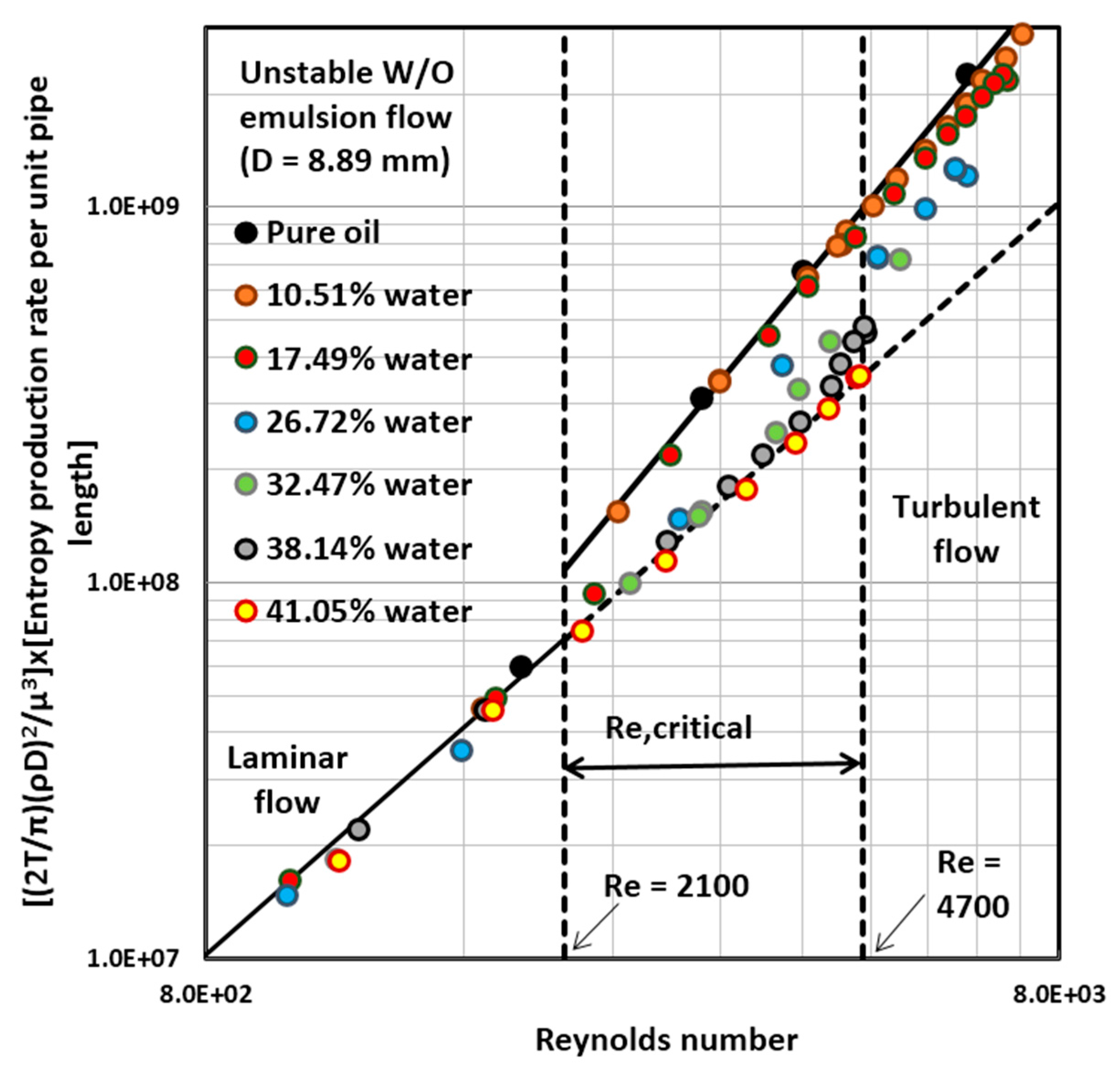
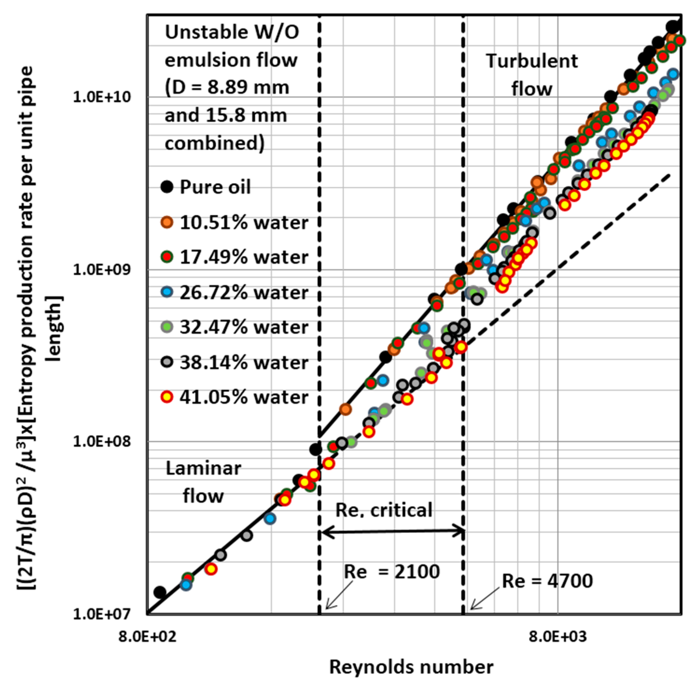
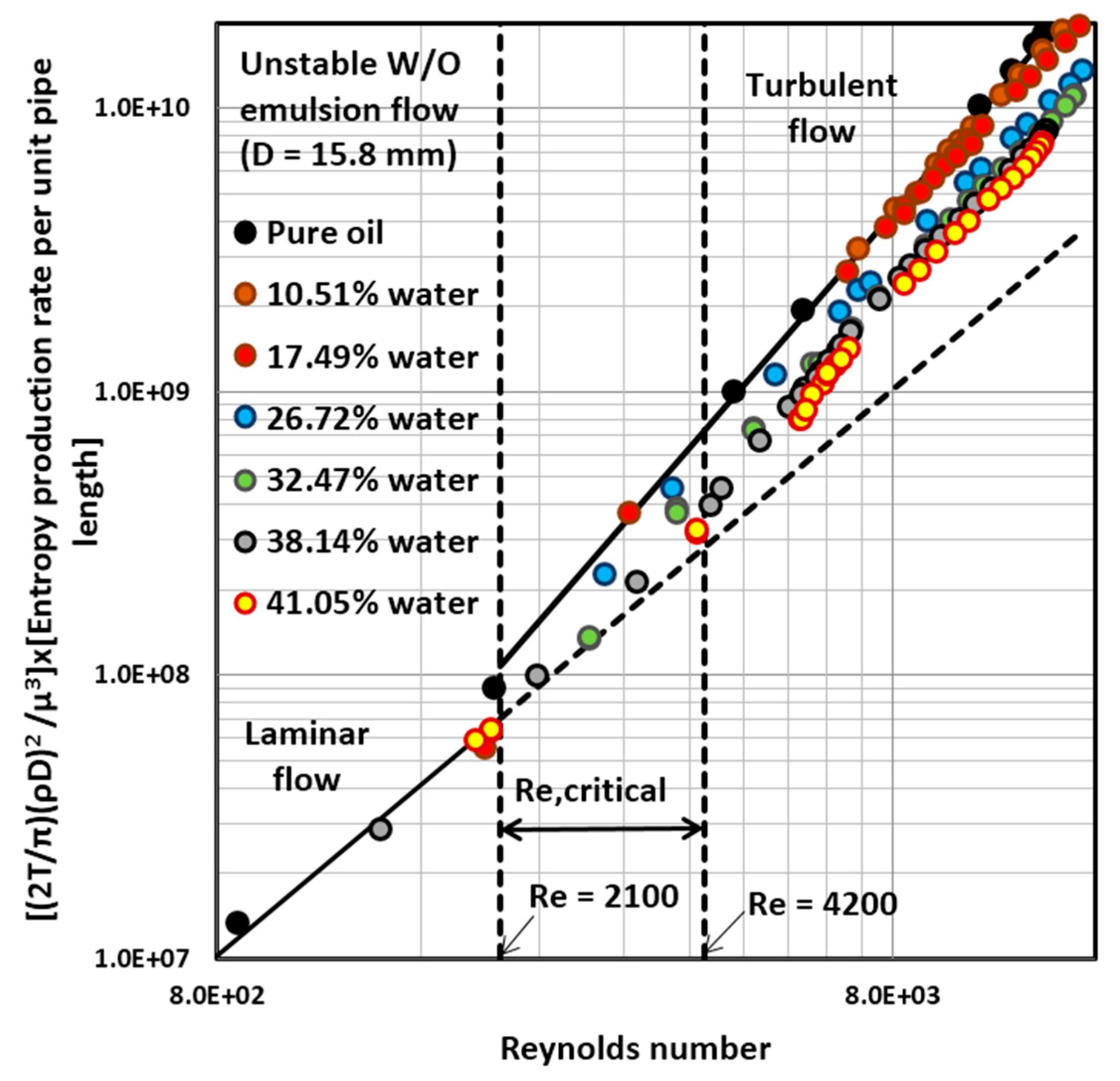
4.3. Entropy Generation in Adiabatic Pipeline Flow of Unstable Water-in-Oil (W/O) Emulsions

The entropy production behavior of unstable W/O emulsions (without any surfactant) is shown in Figure 10. The data are plotted as dimensionless rate of entropy generation ${({\dot{S}}_G^{\prime })}^{\ast }$ versus $\mathrm{Re}$ for differently concentrated unstable W/O emulsions. The data shown in Figure 10 were collected from 8.89 mm diameter pipe. In the laminar regime, the experimental data fall on the line representing Equation (28). However, the turbulent flow data of unstable W/O emulsions exhibit a very different behavior in comparison with the unstable O/W emulsions shown in Figure 4, Figure 5 and Figure 6. The deviation of experimental data from the theoretical line (Equation (29)) is now large. The decrease in friction factor relative to the theoretical line (Equation (29)), and hence drag reduction effect, increases with the increase in the dispersed-phase (water droplets) concentration. Furthermore, the delay in transition from laminar to turbulent regime is magnified. For example, the transition from laminar to turbulent flow occurs at a Reynolds number of approximately 4000 for an emulsion with water concentration of 32.47% by volume. At higher water concentrations, almost complete suppression of turbulence is observed, that is, the experimental data follow the laminar line (Equation (28)) even when the Reynolds number is as high as 4700.

Figure 11 shows ${({\dot{S}}_G^{\prime })}^{\ast }$ versus $\mathrm{Re}$ data for unstable W/O emulsions obtained from a larger diameter pipe (diameter of 15.8 mm). The experimental data from 15.8 mm diameter pipe confirm the observation that unstable W/O emulsions exhibit a strong drag reduction activity in that the experimental data fall well below the theoretical line (Equation (29)). The drag reduction activity increases with the increase in the concentration of water droplets. There also occurs a significant delay in the transition from laminar to turbulent regime.

Figure 12 summarizes the entropy generation behavior of unstable W/O emulsions. All the experimental data obtained from two different diameter pipes for differently concentrated unstable W/O emulsions are shown in Figure 12. Comparison of Figure 12 with Figure 6 clearly brings out the differences in the entropy generation behaviours of unstable (no surfactant) O/W and W/O emulsions. While the unstable O/W emulsions exhibit only a small degree of drag-reduction effect in the turbulent regime, the unstable W/O emulsions are highly drag-reducing in that the entropy generation rates in the turbulent regime are much lower than the theoretical predictions (Equation (29)). Also the delay in laminar to turbulent transition is much larger in the case of unstable W/O emulsions.

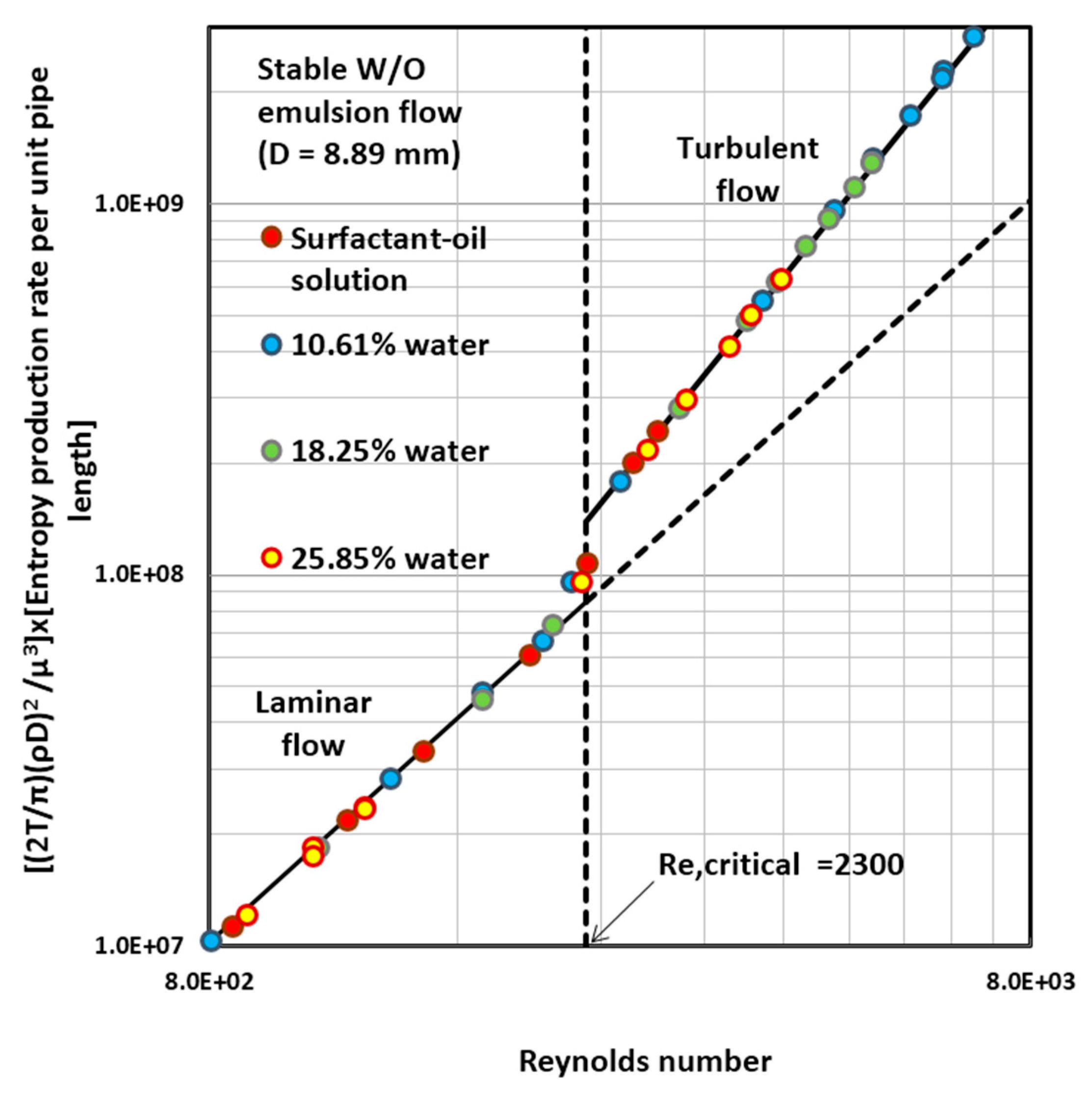
4.4. Entropy Generation in Adiabatic Pipeline Flow of Surfactant-Stabilized Water-in-Oil (W/O) Emulsions

The entropy production behavior of surfactant-stabilized W/O emulsions is shown in Figure 13, Figure 14 and Figure 15. The data are plotted as dimensionless rate of entropy generation ${({\dot{S}}_G^{\prime })}^{\ast }$ versus $\mathrm{Re}$ for differently concentrated surfactant-stabilized W/O emulsions. The data shown in Figure 13 were collected from 8.89 mm diameter pipe whereas the data shown in Figure 14 were collected from a larger diameter (15.8 mm) pipe. In Figure 15, all the experimental data obtained from two different diameter pipes for differently concentrated surfactant-stabilized W/O emulsions are shown.

In the laminar regime, the experimental data fall on the line representing the Equation (28). Surprisingly, the turbulent flow data of surfactant-stabilized W/O emulsions also follow theoretical line (Equation (29)). Thus the addition of surfactant to W/O emulsions completely eliminates the drag reduction behavior exhibited by unstable (without surfactant) W/O emulsions in turbulent flows (see Figure 12). Furthermore, no delay in the transition from laminar to turbulent regime is observed in the presence of surfactant at the surface of the water droplets. The surfactant-stabilized W/O emulsions undergo transition from laminar to turbulent regime at a Reynolds of about 2300. This value is very close to the often-quoted transitional Reynolds number value of 2100 for normal (non drag-reducing) Newtonian fluids.

4.5. Discussion

The surfactant-stabilized emulsions, O/W or W/O type, exhibit normal behavior in that the measured dimensionless rates of entropy generation ${({\dot{S}}_G^{\prime })}^{\ast }$ are in agreement with the theoretical predictions for Newtonian fluids (Equation (28) for laminar regime and Equation (29) for turbulent regime). The unstable emulsions, without any added stabilizer (surfactant), exhibit anomalous behavior under turbulent flow conditions in that the measured dimensionless rates of entropy generation ${({\dot{S}}_G^{\prime })}^{\ast }$ fall well below the theoretical predictions (Equation (29) for turbulent regime). The deviations are particularly large in the case of unstable W/O emulsions. Thus the unstable W/O emulsions are thermodynamically more efficient to pump as compared with the surfactant-stabilized emulsions. In light of the Gouy-Stodola theorem (Equation (19)), the amount of work lost or the unavailable energy associated with pumping of unstable W/O emulsions is the lowest in comparison with other emulsions of equal viscosity and density. A number of factors could be responsible for the observed anomalous behavior of unstable W/O emulsions, including: (i) droplet size; (ii) dynamic coalescence and break-up of droplets; (iii) deformation and stretching of droplets; (iv) elasticity of droplets; (v) viscoelasticity of bulk emulsion; (vi) effective slip at the pipe wall; and (vii) formation of lubricating film at the pipe wall.

The size of the emulsion droplets may be playing a significant role in the suppression of turbulence. The suppression of turbulence is expected when the dispersed water droplets are larger in size than the length scale of turbulence of the carrier fluid. The droplets follow the motion of the turbulent eddies only when they are significantly smaller in size than the turbulent eddies. When the droplets are larger in size than the turbulent eddies, the droplets interfere with the motion of eddies resulting in suppression of turbulence of carrier fluid. Although no attempt was made in this work to measure the droplet sizes in situ, the droplet sizes in unstable (without any added surfactant) emulsions are expected to be significantly larger than the scale of turbulence.

Droplet break-up and coalescence phenomena could be responsible for the anomalous behavior of unstable emulsions in turbulent flow. The droplets of unstable emulsions, without any added interfacial stabilizers, continually undergo coalescence and break-up processes in a turbulent field. The break-up of large droplets into two or smaller droplets extracts energy from the turbulent field resulting in suppression of turbulence and destruction of eddies.

The effective viscosity of emulsions is strongly dependent on the shape of droplets. A sharp reduction in effective viscosity of emulsion is expected in the near wall region upon transition of flow regime from laminar to turbulent due to extensive stretching of droplets in the near wall region in the direction of flow.

The droplets of emulsion possess elasticity of shape because of the restoring force of interfacial tension. Thus the droplets act more like elastic springs capable of absorbing turbulence energy and hence causing a reduction in the intensity of turbulence.

The viscoelasticity of bulk emulsion is another possible mechanism for absorbing turbulence energy resulting in suppression of turbulence. Emulsions tend to be viscoelatic in nature at high concentrations of dispersed phase due to interaction and network structure formation between the droplets.

The anomalous behavior observed in pipeline flow of unstable W/O emulsions could also be explained in terms of effective slip at the pipe wall. The effective slip refers to a pheonomenon whereby the dispersed droplets migrate away from the solid boundaries due to various physico-chemical forces acting on the droplets in the near wall region. Due to the migration of droplets away from the wall region, the wall region is depleted of water droplets resulting in a reduction of emulsion viscosity.

Another possible mechanism causing a reduction in entropy generation rates in unstable W/O emulsion flow is the formation of a thin lubricating film of water on the walls of the pipe. This mechanism is especially important when water droplets have high affinity for the wall material. The water droplets upon contact with the pipe wall spread on the wall forming a thin film of water.

Further experimental studies are needed to pinpoint the mechanism of anomalous behavior of unstable emulsions.

5. Simulation Work: Non-Adiabatic Pipeline Flow of Emulsions

In this section, the non-adiabatic pipeline flow of emulsions is simulated. Emulsions are treated as homogeneous mixtures with average properties. As noted in the preceding section, the surfactant-stabilized emulsions, both O/W and W/O types, indeed behave as homogeneous fluids. The unstable O/W emulsions also approximately follow the homogeneous fluid behavior.

Consider flow of an emulsion in a heated pipeline subjected to a constant wall temperature ($T_b$). The exergy balance (Equation (12)) under steady state condition gives:

$${\dot{\mathsf{\Psi }}}_{D,total}={\dot{\mathsf{\Psi }}}_{D,CV}=\dot{m}{\mathsf{\psi }}_1-\dot{m}{\mathsf{\psi }}_2+{\dot{Q}}_b\left[1-\frac{T_o}{T_b}\right]$$

(30)

where ${\dot{Q}}_b$ is the rate of heat transfer to the fluid at temperature $T_b$, and $T_o$ is the surroundings temperature. Note that exergy destruction in the surroundings is absent. On a unit pipe-length basis, Equation (30) could be re-cast as:

$$\frac{d{\dot{\mathsf{\Psi }}}_{D,total}}{dx}=-\dot{m}\left[\frac{d\mathsf{\psi }}{dx}\right]+{\dot{Q}}_b^{\prime }\left[1-\frac{T_o}{T_b}\right]$$

(31)

where ${\dot{Q}}_b^{\prime }$ is the rate of heat transfer per unit pipe-length. From the First Law of Thermodynamics for open systems (no shaft work, negligible kinetic and potential energy changes):

$$\dot{m}\left(\frac{dh}{dx}\right)={\dot{Q}}_b^{\prime }$$

(32)

From Equations (2) and (32):

$$\frac{d\mathsf{\psi }}{dx}=\frac{{\dot{Q}}_b^{\prime }}{\dot{m}}-T_o\frac{ds}{dx}$$

(33)

Upon combination of Equations (31) and (33), we get:

$$\frac{d{\dot{\mathsf{\Psi }}}_{D,total}}{dx}=\dot{m}{T}_o\left[\frac{ds}{dx}-\frac{{\dot{Q}}_b^{\prime }}{\dot{m}{T}_b}\right]$$

(34)

Using the Gouy-Stodola theorem (Equation (19)), Equation (34) could be re-written as:

$${\dot{S}}_G^{\prime }=\frac{d{\dot{S}}_G}{dx}=\dot{m}\left[\frac{ds}{dx}-\frac{{\dot{Q}}_b^{\prime }}{\dot{m}{T}_b}\right]$$

(35)

where ${\dot{S}}_G^{\prime }$ is the rate of entropy generation per unit length of pipe. Note that there is no entropy generation in the surroundings. For incompressible fluids:

$$\frac{ds}{dx}=\frac{C_p}{T}\frac{dT}{dx}+\frac{1}{\mathsf{\rho }T}\left(-\frac{dP}{dx}\right)$$

(36)

where C_p is the constant-pressure heat capacity of the fluid. From Equations (35) and (36), it follows that:

$${\dot{S}}_G^{\prime }=\left[\left(\frac{\dot{m}{C}_p}{T}\right)\frac{dT}{dx}-\frac{{\dot{Q}}_b^{\prime }}{T_b}\right]+\left[\frac{\dot{m}}{\mathsf{\rho }T}\left(-\frac{dP}{dx}\right)\right]$$

(37)

Upon integration of Equation (37) over the length L of the pipe, the following result is obtained:

$${\dot{S}}_G=\left[\dot{m}{C}_p\ln \left(\frac{T_{out}}{T_{in}}\right)-\frac{{\dot{Q}}_b}{T_b}\right]+\left[\frac{\dot{m}L}{\mathsf{\rho }{T}_{avg}}\left(-\frac{dP}{dx}\right)\right]$$

(38)

where ${\dot{S}}_G$ is the total rate of entropy generation inside the pipe, ${\dot{Q}}_b$ is the total rate of heat transfer to fluid, $T_{out}$ is the mean outlet temperature of the fluid, $T_{in}$ is the mean inlet temperature of the fluid, and $T_{avg}$ is the average temperature of the fluid inside the tube, which can estimated from:

$$T_{avg}=\frac{T_{out}-T_{in}}{\ln \left(\frac{T_{out}}{T_{in}}\right)}$$

(39)

It can be readily shown that:

$$\frac{{\dot{Q}}_b}{T_b}=\frac{\overline{h}(\mathsf{\pi }DL)}{T_b}\mathsf{\Delta }{T}_{lm}$$

(40)

where $\overline{h}$ is the average heat transfer coefficient in the pipe and $\mathsf{\Delta }{T}_{lm}$ is the log-mean temperature, defined as:

$$\mathsf{\Delta }{T}_{lm}=\frac{\mathsf{\Delta }{T}_{out}-\mathsf{\Delta }{T}_{in}}{\ln \left(\frac{\mathsf{\Delta }{T}_{out}}{\mathsf{\Delta }{T}_{in}}\right)}$$

(41)

where $\mathsf{\Delta }{T}_{out}=T_b-T_{out}$, $\mathsf{\Delta }{T}_{in}=T_b-T_{in}$. From Equations (38) and (40), it follows that:

$${\dot{S}}_G=\left[\dot{m}{C}_p\ln \left(\frac{T_{out}}{T_{in}}\right)-\frac{\overline{h}(\mathsf{\pi }DL)}{T_b}\mathsf{\Delta }{T}_{lm}\right]+\left[\frac{\dot{m}L}{\mathsf{\rho }{T}_{avg}}\left(-\frac{dP}{dx}\right)\right]$$

(42)

The second square-bracketed term on the right-hand side of Equation (42) could be further expressed in terms of the friction factor using Equation (26), as given below:

$${\dot{S}}_G=\left[\dot{m}{C}_p\ln \left(\frac{T_{out}}{T_{in}}\right)-\frac{\overline{h}(\mathsf{\pi }DL)}{T_b}\mathsf{\Delta }{T}_{lm}\right]+\left[\frac{32L{\dot{m}}^{3}f}{{\mathsf{\pi }}^2{\mathsf{\rho }}^2{D}^5{T}_{avg}}\right]$$

(43)

The first square-bracketed term on the right-hand side of Equation (43) corresponds to the rate of entropy generation due to irreversible heat transfer to the fluid, and the second square-bracketed term on the right-hand side of Equation (43) corresponds to the rate of entropy generation due to friction in the fluid. Thus:

$${\dot{S}}_G={\dot{S}}_{G,t}+{\dot{S}}_{G,f}$$

(44)

$${\dot{S}}_{G,t}=\left[\dot{m}{C}_p\ln \left(\frac{T_{out}}{T_{in}}\right)-\frac{\overline{h}(\mathsf{\pi }DL)}{T_b}\mathsf{\Delta }{T}_{lm}\right]$$

(45)

$${\dot{S}}_{G,f}=\left[\frac{32L{\dot{m}}^{3}f}{{\mathsf{\pi }}^2{\mathsf{\rho }}^2{D}^5{T}_{avg}}\right]$$

(46)

where ${\dot{S}}_{G,t}$ is the rate of entropy generation due to irreversible heat transfer and ${\dot{S}}_{G,f}$ is the rate of entropy generation due to friction in the fluid. The relative magnitudes of ${\dot{S}}_{G,t}$ and ${\dot{S}}_{G,f}$ in non-adiabatic flow of fluid is often described in terms of the Bejan number (Be), defined as:

$$Be=\frac{{\dot{S}}_{G,t}}{{\dot{S}}_{G,t}+{\dot{S}}_{G,f}}$$

(47)

When Be = 1, the total entropy generated is solely due to irreversible heat transfer and when Be = 0, there is no irreversible heat transfer involved and the total entropy generation is solely due to friction in the fluid.

5.1. Estimation of Friction Factor, Heat Transfer Coefficient, and Outlet Temperature

The flow is assumed to be steady state, hydrodynamically fully developed and thermally developing. In laminar flow of emulsions, the friction factor is estimated from Equation (22). The Blasius equation (Equation (23)) is used for the estimation of friction factor in turbulent flow of emulsions. Equations (22) and (23) are found to be valid for surfactant-stabilized emulsions provided that the emulsions are Newtonian in nature and that the pipeline is hydraulically smooth. The average heat transfer coefficient in thermally developing laminar flow is estimated from the Hausen correlation [17], given below:

$$N\overline{u}=\frac{\overline{h}D}{k}=3.66+\frac{0.0668(D/L)\mathrm{Re}\mathrm{Pr}}{1+0.04{\left[(D/L)\mathrm{Re}\mathrm{Pr}\right]}^{2/3}}$$

(48)

where $N\overline{u}$ is the average Nusselt number, D is pipe diameter, L is pipe length, k is thermal conductivity of fluid, Re is Reynolds number, and Pr is Prandtl number. In turbulent flow of emulsions, the Dittus-Boelter equation is used to estimate the average heat transfer coefficient:

$$N\overline{u}=\frac{\overline{h}D}{k}=0.023{\mathrm{Re}}^{4/5}{\mathrm{Pr}}^{0.4}$$

(49)

The temperature of the fluid leaving the pipe, $T_{out}$, is estimated from the following relation:

$$T_{out}=T_b-\left[\left(T_b-T_{in}\right)\exp \left(-\frac{\mathsf{\pi }DL\overline{h}}{\dot{m}{C}_p}\right)\right]$$

(50)

where $T_b$ is the boundary (wall) temperature.

5.2. Estimation of Thermophysical Properties of Emulsions

For pseudo-homogeneous mixtures of two phases such as emulsions, the density and specific heat capacity can be calculated from the following expressions:

$$\mathsf{\rho }=\mathsf{\phi }{\mathsf{\rho }}_d+\left(1-\mathsf{\phi }\right){\mathsf{\rho }}_m$$

(51)

$$C_p=\frac{\mathsf{\phi }{\mathsf{\rho }}_d{C}_{p,d}+\left(1-\mathsf{\phi }\right){\mathsf{\rho }}_m{C}_{p,m}}{\mathsf{\rho }}$$

(52)

where $\mathsf{\rho }$, ${\mathsf{\rho }}_d$, and ${\mathsf{\rho }}_m$ are the densities of emulsion, dispersed-phase (droplets), and matrix fluid, respectively, $C_p$, $C_{p,d}$, and $C_{p,m}$ are the specific heat capacities of emulsion, dispersed-phase, and matrix fluid, respectively, and $\mathsf{\phi }$ is the volume fraction of the dispersed-phase.

The viscosity of surfactant-stabilized emulsions can be estimated from the following viscosity model of Pal [14,18]:

$$\mathsf{\mu }={\mathsf{\mu }}_m{\left[1-\left\{1+\left(\frac{1-{\mathsf{\phi }}_m}{{\mathsf{\phi }}_m^2}\right)\mathsf{\phi }\right\}\mathsf{\phi }\right]}^{-2.5}$$

(53)

where $\mathsf{\mu }$ and ${\mathsf{\mu }}_m$ are the viscosities of emulsion and matrix fluid, respectively, and ${\mathsf{\phi }}_m$ is the maximum packing volume fraction of particles. For hexagonal close packing of uniform spheres, ${\mathsf{\phi }}_m=0.74$. For polysdisperse emulsions, ${\mathsf{\phi }}_m$ is larger than 0.74, close to about 0.85 [14].

The thermal conductivity of emulsion is estimated from the following Maxwell-Eucken [19] equation:

$$k=k_m\left[\frac{1+2\mathsf{\phi }\left(\frac{\mathsf{\lambda }-1}{\mathsf{\lambda }+2}\right)}{1-\mathsf{\phi }\left(\frac{\mathsf{\lambda }-1}{\mathsf{\lambda }+2}\right)}\right]$$

(54)

where $k$ and $k_m$ are the thermal conductivities of emulsion and matrix fluid, respectively, and $\mathsf{\lambda }$ is the thermal conductivity ratio of dispersed-phase to matrix fluid.

Table 3. Thermophysical properties of the emulsions.

Property	Matrix (Water)	Dispersed-Phase (Oil)	Emulsion $\mathsf{\phi }\mathbf{=}\mathbf{0.20}$	Emulsion $\mathsf{\phi }\mathbf{=}\mathbf{0.30}$	Emulsion $\mathsf{\phi }\mathbf{=}\mathbf{0.40}$	Emulsion $\mathsf{\phi }\mathbf{=}\mathbf{0.50}$	Emulsion $\mathsf{\phi }\mathbf{=}\mathbf{0.60}$
$\mathsf{\rho }(\mathrm{k}\mathrm{g}/{\mathrm{m}}^3)$	1000	780	956	934	912	890	868
Cp(J/(kg·K))	4180	1470	3738	3501	3253	2992	2719
$\mathrm{k}(\mathrm{W}/(\mathrm{m}·\mathrm{K}))$	0.60	0.15	0.488	0.436	0.388	0.343	0.30
$\mathsf{\mu }(\mathrm{m}\mathrm{P}\mathrm{a}·\mathrm{s})$	1	2.5	1.79	2.61	4.13	7.44	16.57
Pr	7	25	14	21	35	65	150

summarizes the thermophysical properties of the emulsions used in the simulations. With the increase in $\mathsf{\phi }$ (dispersed-phase concentration), the density, heat capacity, and thermal conductivity decrease whereas the viscosity and Prandtl number increase.

5.3. Simulation Results and Discussion

To carry out the simulations, the following variables need to be specified in addition to the thermophysical properties: Length (L) and diameter (D) of pipe, , the fluid inlet temperature (T_in) and the wall temperature (T_b). The values of these variables used in the simulations are: L = 0.5 m, D = 1.0 cm, T_in = 293 K, and T_b = 310 K. The thermophysical properties of emulsions are assumed to be approximately constant within the temperature range considered in this work. This is a reasonable approximation as the oulet temperature of the emulsion was within a few degrees of the inlet temperature of 293 K.

Figure 16, Figure 17 and Figure 18 present simulation results for laminar flow of differently concentrated emulsions. The figures show the plots of Bejan number $(Be)$ and the entropy generation rates due to friction $({\dot{S}}_{G,f})$ and irreversible heat transfer $({\dot{S}}_{G,t})$ as functions of Reynolds number (Re). Based on the figures, the following points can be made: (a) the entropy generation rate due to viscous frictional effect in emulsions $({\dot{S}}_{G,f})$ increases with the increase in Re; (b) the entropy generation rate due to irreversible heat transfer to emulsions $({\dot{S}}_{G,t})$ also increases with the increase in Re; (c) ${\dot{S}}_{G,t}$ dominates over ${\dot{S}}_{G,f}$ over the full Re range in the laminar regime; and d) the Bejan number $(Be)$ in laminar flow of emulsions decreases only slightly from a value of unity with the increase in Re. Figure 19 shows the effects of the dispersed-phase concentration $(\mathsf{\phi })$ of emulsion on entropy generation rates, emulsion viscosity, and Bejan number at a fixed Re of 1500. With the increase in $\mathsf{\phi }$, ${\dot{S}}_{G,f}$ increases rapidly whereas ${\dot{S}}_{G,t}$ increases only to a smaller extent although ${\dot{S}}_{G,t}$ still dominates over ${\dot{S}}_{G,f}$. The Bejan number $Be$ decreases only slightly with the increase in $\mathsf{\phi }$. The viscosity of emulsion rises rapidly with the increase in $\mathsf{\phi }$ and therefore, the irreversibility due to viscous frictional effect also rises sharply with the increase in $\mathsf{\phi }$.

Figure 20, Figure 21 and Figure 22 present simulation results for turbulent flow of differently concentrated emulsions. At a low $\mathsf{\phi }$ value of 0.20, the entropy generation rate due to irreversible heat transfer $({\dot{S}}_{G,t})$ still dominates the entropy generation rate due to friction $({\dot{S}}_{G,f})$ over the full Reynolds number range and $Be\approx 1$. However, at high values of $\mathsf{\phi }$, ${\dot{S}}_{G,f}$ dominates over ${\dot{S}}_{G,t}$ and $Be$ decreases substantially with the increase in the Reynolds number.

Figure 23 shows the variations of entropy generation rates with the increase in $\mathsf{\phi }$ at a fixed Reynolds number of 50,000. For $\mathsf{\phi }<0.35$, ${\dot{S}}_{G,t}$ dominates over ${\dot{S}}_{G,f}$ and $Be\approx 1$. At higher values of $\mathsf{\phi }$, ${\dot{S}}_{G,f}$ dominates over ${\dot{S}}_{G,t}$ and the Bejan number $Be$ decreases rapidly with the increase in $\mathsf{\phi }$. The irreversibility due to friction rises sharply with the increase in $\mathsf{\phi }$ due to a rapid increase in the viscosity of the emulsion.

6. Conclusions

Based on the experimental work and second law analysis of adiabatic pipeline flow of emulsions, with and without the presence of surfactant at the droplet interface, the following conclusions can be made: (a) in the absence of any surfactant at the droplet interface, the unstable emulsions generate less entropy as compared with single-phase Newtonian fluids of the same viscosity and density in the turbulent regime. This indicates that pumping of unstable emulsions is more efficient thermodynamically provided that the flow regime is turbulent; (b) the entropy generation rate in unstable water-in-oil (W/O) emulsions is significantly lower than that in unstable oil-in-water (O/W) emulsions; (c) the surfactant-stabilized emulsions, regardless of the type (W/O or O/W), behave like truly homogeneous fluids in that the entropy generation rates are in agreement with the corresponding values for single-phase Newtonian fluids of the same viscosity and density. Based on the simulation work and second law analysis of non-adiabatic flow of emulsions, it can be concluded that: (a) in laminar pipeline flow of emulsions, the entropy generation is mainly due to irreversible heat transfer to emulsions. With the increase in the dispersed-phase concentration, the entropy generation rate due to friction rises more rapidly than the entropy generation rate due to irreversible heat transfer; and (b) in turbulent pipeline flow of emulsions, the main contribution to entropy generation comes from frictional effects over the whole range of Reynolds number at high concentrations of dispersed-phase.

References

1. Energy Efficiency Guide for Industry in Asia, Energy Equipment: Pump and Pumping Systems, United Nations Environment Programme 2006. Available online: http: //www.energyefficiencyasia.org (accessed on 17 December 2015).
2. Smith, J.M.; van Ness, H.C.; Abbott, M.M. Introduction to Chemical Engineering Thermodynamics, 7th ed.; McGraw-Hill: New York, NY, USA, 2005; pp. 635–636. [Google Scholar]
3. Abbott, M.M.; van Ness, H.C. Theory and Problems of Thermodynamics, Schaum’s Outline Series, 2nd ed.; McGraw-Hill: New York, NY, USA, 1989; pp. 302–307. [Google Scholar]
4. Cengel, Y.; Boles, M. Thermodynamics: An Engineering Approach, 7th ed.; McGraw-Hill: New York, NY, USA, 2011. [Google Scholar]
5. Bejan, A. Entropy Generation through Heat and Fluid Flow; Wiley & Sons: New York, NY, USA, 1982; pp. 105–107. [Google Scholar]
6. Pal, R. Rheology of Particulate Dispersions and Composites; CRC Press: Boca Raton, FL, USA, 2007. [Google Scholar]
7. Pal, R. Effect of droplet size on the rheology of emulsions. AIChE J. 1996, 42, 3181–3190. [Google Scholar] [CrossRef]
8. Pal, R. Pipeline flow of unstable and surfactant-stabilized emulsions. AIChE J. 1993, 39, 1754–1764. [Google Scholar] [CrossRef]
9. Pal, R.; Rhodes, E. Emulsion flow in pipelines. Int. J. Multiph. Flow 1989, 15, 1011–1017. [Google Scholar] [CrossRef]
10. Pal, R. On the flow characteristics of highly concentrated oil-in-water emulsions. Chem. Eng. J. 1990, 43, 53–57. [Google Scholar] [CrossRef]
11. Pal, R. Rheology of simple and multiple emulsions. Curr. Opin. Colloid Interface Sci. 2011, 16, 41–60. [Google Scholar] [CrossRef]
12. Pal, R. Techniques for measuring the composition (oil and water content) of emulsions—A state of the art review. Colloids Surfaces A 1994, 84, 141–193. [Google Scholar] [CrossRef]
13. Pal, R. Entropy production in pipeline flow of dispersions of water in oil. Entropy 2014, 16, 4648–4661. [Google Scholar] [CrossRef]
14. Pal, R. Exergy destruction in pipeline flow of surfactant-stabilized oil-in-water emulsions. Energies 2014, 7, 7602–7619. [Google Scholar] [CrossRef]
15. Pal, R. Entropy generation in flow of highly concentrated non-Newtonian emulsions in smooth tubes. Entropy 2014, 16, 5178–5197. [Google Scholar] [CrossRef]
16. Bejan, A. Entropy Generation Minimization: The Method of Thermodynamic Optimization of Finite-Size Systems and Finite-Time Processes; CRC Press: Boca Raton, FL, USA, 1996. [Google Scholar]
17. Bergman, T.L.; Lavine, A.S.; Incropera, F.P.; Dewitt, D.P. Fundamentals of Heat and Mass Transfer, 7th ed.; John Wiley & Sons: New York, NY, USA, 2011. [Google Scholar]
18. Pal, R. New models for the viscosity of nanofluids. J. Nanofluids 2014, 3, 260–266. [Google Scholar] [CrossRef]
19. Pal, R. Electromagnetic, Mechanical, and Transport Properties of Composite Materials; CRC Press: Boca Raton, FL, USA, 2015. [Google Scholar]
Figure 1. Non-adiabatic flow in a pipe.
Entropy 18 00113 g001
Figure 2. Heat reservoirs are placed directly at the control volume boundary such that the temperature at the boundary is the same as that of the heat reservoir.
Entropy 18 00113 g002
Figure 3. Carnot heat engines placed between the control volume boundary and heat reservoirs.
Entropy 18 00113 g003
Figure 4. Dimensionless rate of entropy generation ( S ˙ G ) versus Re data for differently concentrated unstable O/W emulsions, without the presence of any surfactant, obtained from a pipe of diameter 8.89 mm.
Entropy 18 00113 g004
Figure 5. ( S ˙ G ) versus Re data for unstable O/W emulsions obtained from a pipe of diameter of 15.8 mm.
Entropy 18 00113 g005
Figure 6. All the experimental data for differently concentrated unstable O/W emulsions obtained from two different diameter pipes.
Entropy 18 00113 g006
Figure 7. Dimensionless rate of entropy generation ( S ˙ G ) versus Re data for differently concentrated surfactant-stabilized O/W emulsions obtained from a pipe of diameter 8.89 mm.
Entropy 18 00113 g007
Figure 8. ( S ˙ G ) versus Re data for surfactant-stabilized O/W emulsions obtained from a pipe of diameter of 15.8 mm.
Entropy 18 00113 g008
Figure 9. All the experimental data for differently concentrated surfactant-stablized O/W emulsions obtained from two different diameter pipes.
Entropy 18 00113 g009
Figure 10. Dimensionless rate of entropy generation ( S ˙ G ) versus Re data for differently concentrated unstable W/O emulsions, without the presence of any surfactant, obtained from a pipe of diameter 8.89 mm.
Entropy 18 00113 g010
Figure 11. ( S ˙ G ) versus Re data for unstable W/O emulsions obtained from a pipe of diameter of 15.8 mm.
Entropy 18 00113 g011
Figure 12. All the experimental data for differently concentrated unstable W/O emulsions obtained from two different diameter pipes.
Entropy 18 00113 g012
Figure 13. Dimensionless rate of entropy generation ( S ˙ G ) versus Re data for differently concentrated surfactant-stabilized W/O emulsions obtained from a pipe of diameter 8.89 mm.
Entropy 18 00113 g013
Figure 14. ( S ˙ G ) versus Re data for surfactant-stabilized W/O emulsions obtained from a pipe of diameter of 15.8 mm.
Entropy 18 00113 g014
Figure 15. All the experimental data for differently concentrated surfactant-stabilized W/O emulsions obtained from two different diameter pipes.
Entropy 18 00113 g015
Figure 16. Variation of entropy generation rates ( S ˙ G , f and S ˙ G , t in units of J/(K·s)) and Bejan number ( B e ) with Reynolds number in laminar flow of emulsion ( φ = 0.20).
Entropy 18 00113 g016
Figure 17. Variation of entropy generation rates ( S ˙ G , f and S ˙ G , t in units of J/(K·s)) and Bejan number ( B e ) with Reynolds number in laminar flow of emulsion ( φ = 0.50).
Entropy 18 00113 g017
Figure 18. Variation of entropy generation rates ( S ˙ G , f and S ˙ G , t in units of J/(K·s)) and Bejan number ( B e ) with Reynolds number in laminar flow of emulsion ( φ = 0.60).
Entropy 18 00113 g018
Figure 19. Variation of entropy generation rates ( S ˙ G , f and S ˙ G , t in units of J/(K·s)), viscosity ( μ in units of Pa·s) and Bejan number ( B e ) with φ in laminar flow of emulsions at a fixed Re of 1500.
Entropy 18 00113 g019
Figure 20. Variation of entropy generation rates ( S ˙ G , f and S ˙ G , t in units of J/(K·s)) and Bejan number ( B e ) with Reynolds number in turbulent flow of emulsion ( φ = 0.20).
Entropy 18 00113 g020
Figure 21. Variation of entropy generation rates ( S ˙ G , f and S ˙ G , t in units of J/(K·s)) and Bejan number ( B e ) with Reynolds number in turbulent flow of emulsion ( φ = 0.50).
Entropy 18 00113 g021
Figure 22. Variation of entropy generation rates ( S ˙ G , f and S ˙ G , t in units of J/(K·s)) and Bejan number ( B e ) with Reynolds number in turbulent flow of emulsion ( φ = 0.60).
Entropy 18 00113 g022
Figure 23. Variation of entropy generation rates ( S ˙ G , f and S ˙ G , t in units of J/(K·s)), viscosity ( μ in units of Pa·s) and Bejan number ( B e ) with φ in turbulent flow of emulsions at a fixed Re of 50,000.
Entropy 18 00113 g023