Article

Off-Design Modeling of Natural Gas Combined Cycle Power Plants: An Order Reduction by Means of Thermoeconomic Input–Output Analysis

by
Sajjad Keshavarzian
*,†,
Francesco Gardumi
,
Matteo V. Rocco
and
Emanuela Colombo
Department of Energy, Politecnico di Milano, Via Lambruschini 4, 20156 Milan, Italy
*
Author to whom correspondence should be addressed.
These authors contributed equally to this work.
Entropy 2016, 18(3), 71; https://doi.org/10.3390/e18030071
Submission received: 10 September 2015 / Revised: 5 February 2016 / Accepted: 10 February 2016 / Published: 26 February 2016
(This article belongs to the Special Issue Thermoeconomics for Energy Efficiency)

Abstract

:
In a European context characterized by growing need for operational flexibility across the electricity sector, the combined cycle power plants are increasingly subjected to cyclic operation. These new operation profiles cause an increase of production costs and decrease of revenues, which undermines the competitiveness of the combined cycles. Power plant operators need tools to predict the effect of off-design operation and control mechanisms on the performance of the power plant. Traditional Thermodynamic or Thermoeconomic models may be unpractical for the operators, due to their complexity and the computational effort they require. This study proposes a Thermoeconomic Input–Output Analysis model for the on- and off-design performance prediction of energy systems, and applies it to La Casella Natural Gas Combined Cycle (NGCC) power plant, in Italy. It represents a stand-alone, reduced order model, where the cost structure of the plant products and the Thermoeconomic performance indicators are derived for on- and off-design conditions as functions of the load and of different control mechanisms, independently from the Thermodynamic model. The results of the application show that the Thermoeconomic Input–Output Analysis model is a suitable tool for power plant operators, able to derive the same information coming from traditional Thermoeconomic Analysis with reduced complexity and computational effort.

1. Introduction

According to the guidelines of EU Energy Roadmap 2050, Natural Gas Combined Cycle (NGCC) power plants may become the main backup technology in the low carbon European electricity system [1]. Following the current trend, the average capacity factor may decrease while the amplitude of load variations, the number of ramp-up cycles, and their steepness increase. This implies that NGCCs may experience an increase of production costs and decrease of revenues, which undermines their competitiveness and possibly the adequacy of the grid. Therefore, the operators are interested in lowering the generation costs and benefitting from price peaks on the market, in order to regain competitiveness. This can be attained by modifying the configuration of the power plants and the operation strategies, so as to enhance the cycling capability of the units [2,3]. However, the operators hardly have tools to predict the benefits deriving from new configurations or control logics. On one side, the live monitoring systems of the power plants only measure and record the present thermodynamic quantities, taking snapshots of the performance, without any predictive capability. On the other side, the thermodynamic models in literature for the performance evaluation of NGCCs seem to be more research-oriented than industry-oriented, requiring complex solution algorithms and often high computational time and effort.

1.1. State-of-the-Art Performance Evaluation of NGCC Power Plants

Several thermodynamic models have been proposed for the off-design performance prediction of power plants. Dynamic models are usually employed to assess the performance and the potential improvements on specific components, like those computing the response time of the Heat Recovery Steam Generator (HRSG) to thermal transients [4]. Quasi-stationary models are useful to compute the thermodynamic benefits of given interventions over time averaged profiles [5,6,7,8,9]. Techno-economic methodologies add cost accounting evaluations to the thermodynamic performance predictions, providing the operators with more complete pictures of the potential costs and benefits. However, they do not pinpoint the causes for cost increases in off-design operation, because they do not look into the productive structure of the processes [10]. Literature suggests Thermoeconomic Analysis (TA) as an appropriate tool to evaluate the cost structure of energy system products, allowing internal evaluations on the performance of each component in off-design operation [11]. TA pertains to the domain of Exergy Analysis (ExA), which can be considered one of the most famous and employed tools in the field of energy system analysis [12,13,14].
Kotas et al. introduced the concept of structural coefficients to estimate to what extent the variation of the efficiency of a component in a chain influences another component in that chain [12]. This is a key concept in the industrial practice, since it allows the analyst to compute and locate the inefficiencies in the power plant and, consequently, to predict the benefits of new configurations or control mechanisms [15,16]. Valero et al. provided a synthesis of this concept introducing the Input–Output approach for Thermoeconomic Analysis of generic systems [17,18,19]. Input–Output is well established in economics to analyze the interaction between economic sectors, producers, and consumers [20]; applied to the performance analysis of power plants, it provides a picture of the relationships between resources and products of the various components. So far, this approach has been applied only to the on-design performance evaluation.
One weakness of all these models is that they are often more research-oriented than industry-oriented and their indications for the performance optimization cannot be implemented by the power plant operators [20,21]. In the first place, some suggest interventions on components which can hardly be changed: in an existing power plant, components such as the compressor, the combustion chamber or entire heat exchangers will not be easily replaced, or major interventions on the gas turbine will not be carried out off-schedule. On the contrary, the on- and off-line cleaning procedures of components like compressor, condenser and heat exchangers may be re-scheduled upon the indications coming from Thermoeconomic Analyses. Secondly, disaggregated information on some components (such as the gas turbine assembly) may be useless for the operators, when they have limited margin to improve them; conversely, it may be crucial on other components, when the malfunctions can be repaired with minor maintenance interventions (such as fouling on heat exchangers in the HRSG). Another weakness is the complexity of the models and the high computational effort and time they require, which may make them unfit to be directly employed by industrial practitioners. This may cause barriers between scientific research and industrial practice to arise. Barriers for the operators arise, since they cannot employ these models to predict the performance of the power plants with new configurations or control mechanisms; barriers for the researchers arise, who cannot apply their models to case studies of interest for the operators and draw indications about feasible improvements.

1.2. Objective and Structure of the Work

The present work proposes a Thermoeconomic Input–Output Analysis (TIOA) model for the on- and off-design performance prediction of energy systems, and applies it to La Casella NGCC power plant, operating in northern Italy.
This work contributes to the state-of-the-art literature and current industrial practice in the following ways:
  • It is a stand-alone and reduced order model: by means of Input–Output mathematics, it computes the costs of the products and other thermoeconomic parameters independently from the thermodynamic plant model. The reduced complexity and computational effort of TIOA may help abate the aforementioned barriers between scientific research and industrial practice;
  • It can be applied for the analysis of many different on- and off-design plant configurations and control mechanisms, providing useful indications to power plant operators for the purposes of cost assessment, design optimization or malfunction diagnosis.
In Section 2, Section 3 and Section 4, the derivation of the Thermodynamic, Cost and TIOA models is respectively described. In Section 5, the on- and off-design TIOA model is applied to the considered power plant.

2. Materials and Methods

The novel TIOA approach proposed by the Authors is here presented.

2.1. Thermoeconomic Input Output Analysis

Let us consider one generic energy system composed of n pieces of equipment, connected to each other and to the environment by m material and energy interactions characterized by means of their exergy equivalents. Exergy can be defined as “the amount of useful work extractable from a generic system when it is brought to equilibrium with its reference environment through a series of reversible processes in which the system can only interact with such environment” [12]. All the exergy flows can be classified according to their economic purpose, through the so-called Resource-Product-Losses (RPL) criterion [22]: this practice allows the analyst to distinguish among productive components, whose main purpose is to generate a useful product, and dissipative components, that do not generate any final product, but are responsible for disposing of the residues created during production (condensers, filters, scrubbers, stacks, etc.).
Therefore, n exergy balances and exergy efficiencies can be defined as in relation Equation (1). Note that this definition is not unique and depends on the component and its operational role within the system,
E ˙ x R , i = E ˙ x P , i + E ˙ x L , i + E ˙ x D , i η i = E ˙ x P , i E ˙ x R , i .
According to the theoretical formulation of TIOA, given that the material and energy flows within the system are properly classified based on the RPL criterion, the definition of the auxiliary relations which was necessary for the traditional approach (incidence matrix representation) [23], is implicitly included in the Input–Output analysis and no longer required.
Let the generic system be composed of n P productive components P ( 1 , , n P ) and n D dissipative components D ( n P + 1 , , n P + n D ) , with   n = n P + n D . For this system, the Transaction matrix Z is defined, whose elements represent the exergy rate (J/s) produced by ith component and fueled as a resource to jth component,
Z = [ E ˙ x P , i j ] i , j P D .
The definition of exergy junction ratios is required to overcome the problem of allocating the product of multiple components as a resource of other components [17,24]. The amount of exergy provided to the environment by productive and dissipative components is respectively collected in the Final Demand vector f ( n P × 1 ) and in the Residue vector g ( n D × 1 ) : these vectors define the System Output vector w ( n × 1 ) according to relation Equation (3),
w = [ f ( n P × 1 ) g ( n D × 1 ) ] { f = [ E ˙ x P , i 0 ] i P g = [ E ˙ x L , i 0 ] i D .
The Resource vector R ( n × 1 ) collects the amount of exogenous resources that directly fuel the system. Its elements can be defined in different units, leading to the definition of different costs of the final demand   f : in Exergy Cost Theory (ECT) and Exergoeconomic Cost Analysis, the elements of R represent respectively the exergy (in J/s) and the economic cost (in €/s) provided to each component. In this article, the Resource vector R is compiled in monetary units, and it includes fuel costs, capital investment and depreciation, as well as operation and maintenance expenses, allocated among all the n components.
The Technical Coefficients matrix A ( n × n ) and the Input vector B ( n × 1 ) are defined according to standard Input–Output analysis (IOA) as in relation Equation (4),
A = Z x ^ 1      ;      B = R x ^ 1 .
Thanks to the introduced definitions, it is possible to evaluate the specific and total exergy and economic costs of both system products and residues, according to Equation (5), where c ( n × 1 ) is the specific cost vector, C ( n × 1 ) is the total cost vector, and L ( n × n ) is the Leontief Inverse matrix. In IOA, relation Equation (5) is known as the Leontief Cost Model (LCM) [25],
L = ( I A ) 1           c = L T B           C = w ^ c .
According to the cost accounting practice, the cost of the residues should be reallocated to useful products only. This can be done through the proportionality criterion proposed by Valero [17,26]: the cost of the residue of the jth dissipative component is allocated to each productive component that feeds it, in proportion to the amount of exergy it delivers to j. This is expressed by the residues cost distribution ratio   ψ j i , defined by Equation (6) as the fraction of jth resource coming from the ith component,
ψ j i = E ˙ x P , i j E ˙ x R , j           i P ψ j i = 1      i P , j D .
A Residues production coefficients matrix W R ( n × n ) can be thus defined to collect the residues production coefficients   ρ j i   , defined in matrix form by relation Equation (7),
W R = [ ρ j i ]         ρ j i = { 0 j P ψ j i E ˙ x P , j E ˙ x P , i j D .
Rearranging the cost balances and introducing Equations (6) and (7), the reallocated specific and total exergy costs of useful products only can be determined as in relation Equation (8),
L = ( I A W R ) 1         c ' = L R T B        C ' = w ^ c ' .
The systems of equations introduced above in matrix form can be schematically represented as in Figure 1.
Apart from the specific exergy cost of plant products, the standard exergy cost evaluation formalized here leads to the definition of a set of parameters which allow the so-called iterative design evaluation and optimization process, as described by [17,19,22]:
  • Exergy destruction and losses: defined by Equation (9), they reveal the location and the magnitude of the thermodynamic irreversibilities within each component. Vector i is known as summation vector [27]
    E ˙ x R , i = E ˙ x P , i + E ˙ x L , i + E ˙ x D , i D = ( i 1 × n Z ) T Z i n × 1 .
  • Exergoeconomic costs of exergy destructions: defined by Equation (10), they reveal the impact that the thermodynamic inefficiencies occurring in each component have on the economic costs of the products.
    C E x D = D ^ c

2.2. Derivation of the Stand-Alone Thermoeconomic Input–Output Model

In this section, a procedure to derive a TIOA model is defined by the Authors:
  • Thermodynamic modelling and simulation. The performance of the power plant in off-design operation depends on many parameters, and these may be classified into two main groups: exogenous parameters, which are not controlled by the operator (such as environmental temperature or LHV of the fuel), and endogenous parameters, which can be controlled (such as load control mechanism, plant load and the reversible performance degradation of one or more components by means of maintenance interventions).
    The response of the power plant to different values of each of these parameters can be evaluated by running the thermodynamic model several times. However, this carries some drawbacks: it involves time and computational effort; it provides results only for discrete values of the parameters; and, most of all, it requires expertise in thermodynamic modeling. In the most general case, a number K of exogenous or endogenous parameters can be considered. Assuming a number α i of possible values for each ith parameter, a total number of plant simulations N S must be performed according to relation Equation (11),
    N s = i = 1 K α i .
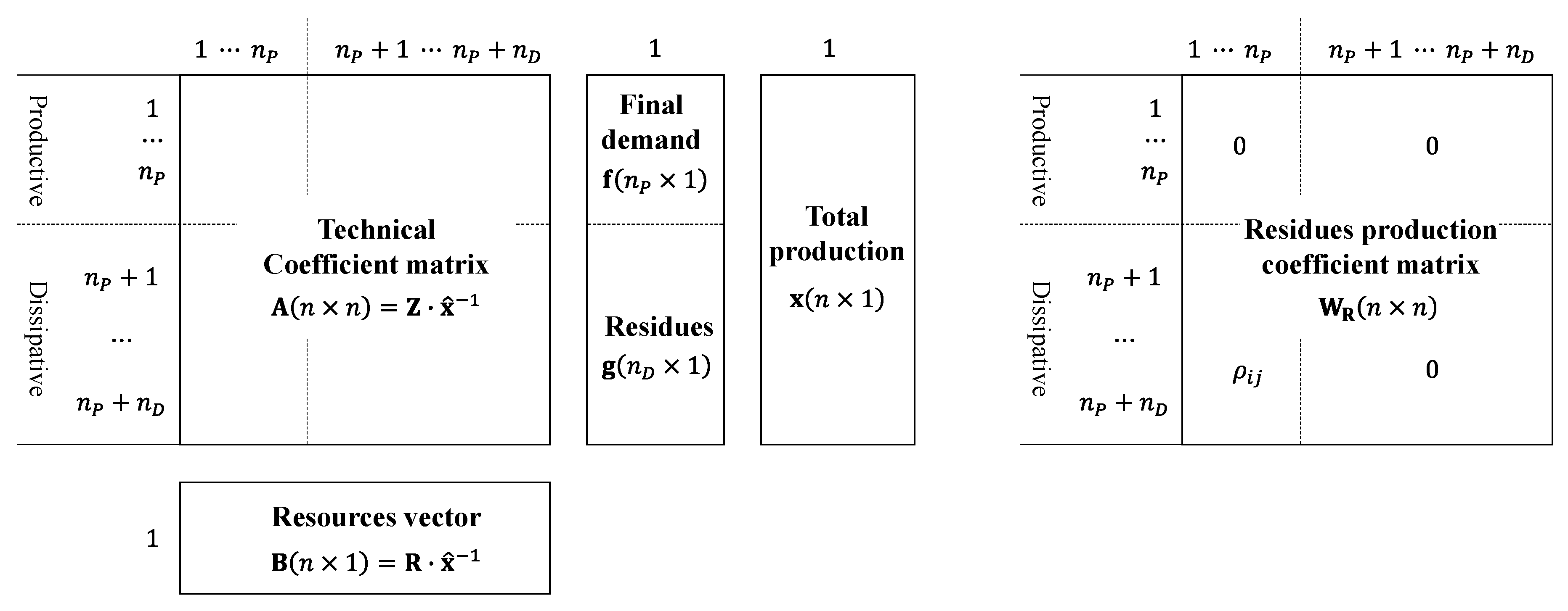
  • Exergy and TIOA analysis. Both the on- and off-design model computed temperature, pressure and mass flow rate of each stream at different operating conditions. From such values, the related exergy rates are derived according to literature [12,22,28], and exergy balances for each plant component are derived according to relation Equation (1). The fundamental matrices and vectors presented in Figure 1 are then derived for each on- and off-design configuration of the system, as described in Subsection 2.1. Finally, the specific and total exergoeconomic costs are derived through LCM Equation (8), as well as the exergy destructions Equation (9) and the exergoeconomic costs of exergy destructions Equation (10);
  • Definition of the stand-alone TIOA model. Each element in the matrices and vectors of Figure 1 is derived as a continuous function of the above introduced endogenous and exogenous variables through linear regression, by means of a Visual Basics® (Microsoft Visual Basic for applications 7.0, Version 1628) procedure implemented by the Authors. These results in a reduced order Thermoeconomic model of the power plant: LCM Equation (8) can be applied to a single functional input–output table where the only inputs are the values of the endogenous/exogenous parameters of interest, and the outputs are the performance indices of the power plant, from the global to the component level.

3. Case Study: La Casella NGCC

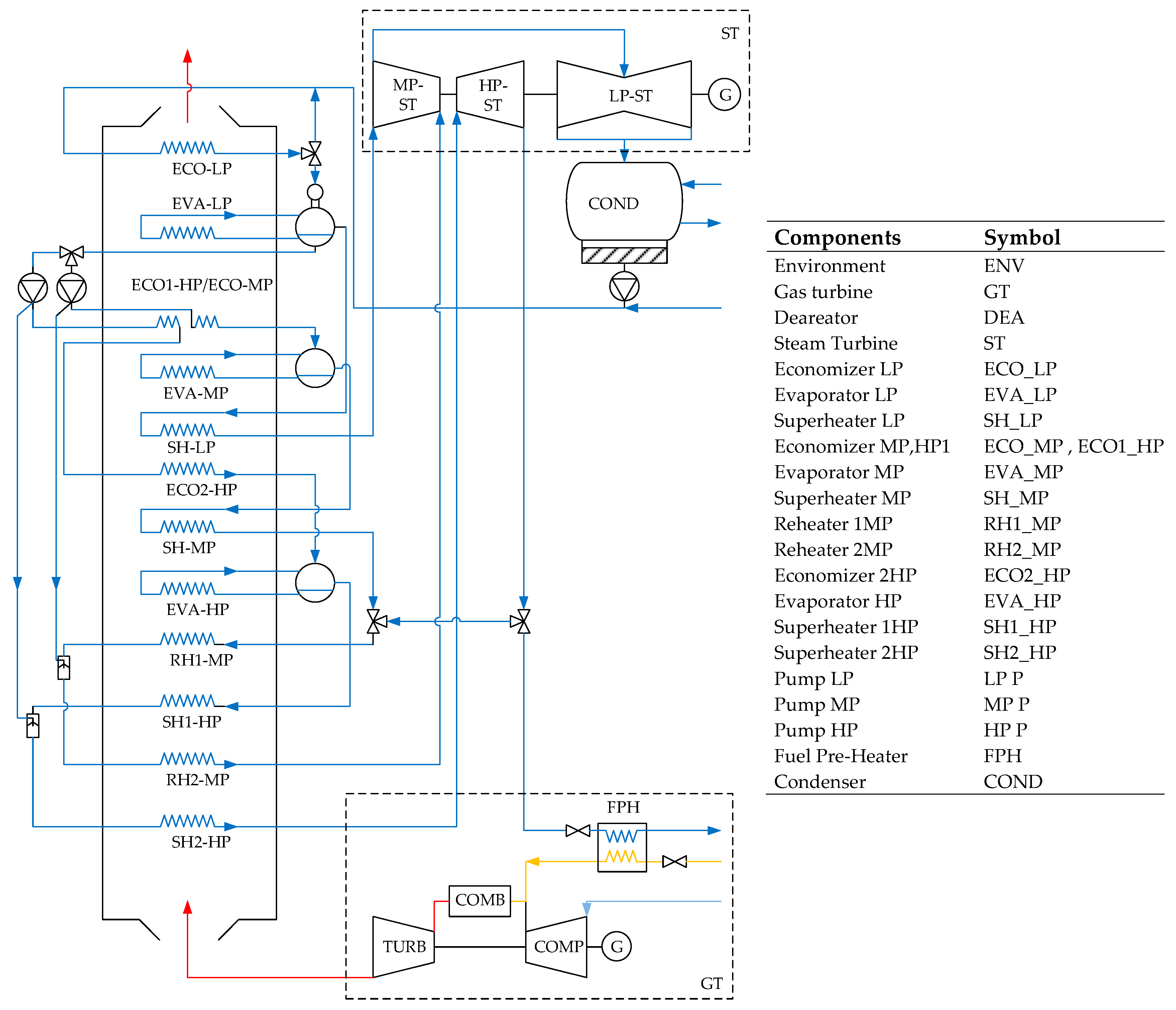
3.1. Thermodynamic Model: Plant Layout and Main Assumptions

The NGCC power plant of La Casella (PC), operated by Enel S.p.A. in northern Italy, is considered: it consists of four groups, each made of one gas turbine and a coupled vertical HRSG (repowered from a boiler). Since the groups are identical, the analysis is performed only for one of them, represented in Figure 2. The software Thermoflow Thermoflex™ (Version 24.1.1, Revision: 23 September 2014) is employed to perform the thermodynamic simulation of the plant in both on- and off-design conditions: it is a zero-dimensional software for power plant modeling, which iteratively solves the mass and energy balances at the nodes of a network of pre-defined or user-defined components.
Common inputs. The analyzed plant consists of the following main components: gas turbine (GT), which generates a design net electric power of 252.5 MW with a turbine inlet temperature (TIT) of 1295.6 °C; HRSG with 13 heat exchangers operating on three pressure levels; steam turbine (ST) with design 131.5 MW electric power generation; and condenser (COND). For the gas turbine assembly, a model of Siemens V94.3a is available in the database of Thermoflex. It is employed in the model for it to adhere as much as possible to the real power plant. However, this prevents knowledge of the maps of the turbine and the compressor, because they are not released by the manufacturer. Moreover, the so modeled gas turbine is almost a black box, not split into its individual components. In the present case, Siemens V94.3a serves the purpose of the study to show a new modeling approach, but it can easily be replaced when needed. As far as the steam turbine is concerned, it consists in high, intermediate and low pressure bodies, of eleven, four and six stages, respectively. The maps of the bodies are not known as well. However, the turbines operate in sliding pressure control; therefore, their efficiencies can be considered constant [29].
Inputs to the on-design model. In addition to the common inputs, the pinch points of the evaporators, the sub-cooling temperatures of the economizers, the steam outlet temperatures of the super-heaters are fixed for each pressure level. Figure 3 shows the T-Q diagram of the HRSG in design conditions. The length of the lines on the horizontal axis shows the transferred heat rate and the vertical axis shows the temperature levels. Since, in the parallel economizers (ECO1-HP and ECO-MP), heat is exchanged simultaneously between one stream of flue gases and two streams of water, the heat transferred in each economizer cannot be illustrated properly in the T-Q diagram. Therefore, in order to distinguish the heat duty of each heat exchanger, the parallel economizers are shown in series. The numbers below the specified heat exchangers in Figure 3 are the transferred heat to the water side in kW. Starting from all these inputs, the mass and energy balance equations of the system are closed, the remaining properties of all the streams are computed and the geometric features of the components are derived. The on-design model is validated by comparison of the results with the operation data available from the power plant.
Inputs to the off-design model. In the off-design model, the geometric characteristics of the components derived in the previous simulation become inputs. The present study focuses on the effects of cycling operation on the performance of the power plant. Therefore, endogenous variables like gas turbine load, off-design control mechanisms and performance decay of some components become inputs. The steam turbines work in sliding pressure: therefore, the load of the whole power plant is controlled through the gas turbine by closure of the compressor’s Inlet Guide Vanes (IGVs). When the valves are completely closed, the load of the gas turbine is reduced to 50% of the nominal load. When the air mass flow rate is reduced through the IGVs, the fuel flow rate is also reduced according to two control mechanisms:
  • Constant Turbine Outlet Temperature (TOT). This reduces the thermal stresses over the heat exchangers in the bottoming cycle in off-design, and the TIT decreases consequently;
  • Constant Turbine Inlet Temperature (TIT). This is claimed to limit the global reduction of efficiency. The TOT increases, but the parts of the HRSG exposed to the highest temperatures are safe, since they were originally sized for a simple steam cycle, with higher temperatures.
Notice that the two control mechanisms introduced above represent two limit conditions; in real operation, hybrid mechanisms combining these two may be employed as well. The impact of exogenous variables like the environmental conditions or the LHV of the fuel can be easily evaluated with the model, but this is outside the scope of the present work. Thus, they are assumed to be fixed in all the simulations. The properties of all the streams are now dependent variables and they are computed at different loads of the gas turbine, from 100% to 50% by steps of 5%. A macro is defined in Thermoflow Thermoflex™ for this purpose. Moreover, they are computed for both the control mechanisms of the gas turbine, TIT and TOT, by fixing its settings in the model. The off-design model is validated by comparison with the on-design model at 100% load of the gas turbine.
The main inputs of the on- and off-design models are listed in Table 1.

3.2. Economic Cost Model

The economic model is based on the Total Revenue Requirement (TRR) method, described by Bejan et al. in [14]. The Purchased Equipment Costs (PECs) are based on the industrial database of Thermoflow Thermoflex™ and they are listed in Table 2. The remaining cost items are computed as a percentage of the total PEC.
In line with Cafaro et al., the aggregated costs of the steam turbine and of the pumps are allocated to the single components proportionally to the mechanical power, respectively delivered and absorbed; similarly, the global cost of the HRSG is allocated to each heat exchanger proportionally to the thermal power transferred [32]. Concerning the operating and maintenance expenses (O&M) of the power plant, they are aggregated together with many other cost items, making it difficult to retrieve reliable information. Therefore, this cost item is obtained through industrial literature review [32,33,34]. Errors in the value may bias the computation of the specific costs, but they will not affect the comparative evaluations. The yearly fixed O&M costs amount to 15.37 €/kW, while the variable O&M costs amount to 3.27 €/MWh [34], and they are allocated to the components proportionally to their PEC, according to Bejan et al. [14]. It is assumed that 2002 is the year of the evaluation: thus, all costs are computed in €2002. The actual production schedule of the case study power plant is obtained from the databank of Italian Gestore dei Mercati Energetici [35], and it refers to average cycling operation. The yearly equivalent operating hours are approximately obtained by considering those of a sample week and multiplying them by the number of weeks in a year. The result is 3566 h, corresponding to a mid-merit operation profile.
Considering the economic parameters listed in Table 3, a Total Revenue Requirement (TRR) value of 9.474 current M€ is computed, of which 7.268 M€ is the cost for the fuel. The levelized cost is hence computed, and it is allocated to each component proportionally to its PEC. Fixed values of the specific levelized costs are obtained.

3.3. NGCC Stand-Alone Thermoeconomic Input–Output Model

In order to apply TIOA, the physical structure of the power plant is simplified as in Figure 4. All the exergy fluxes are grouped according to the RPL criterion and the functional diagram of the plant is derived, as depicted in Table 4.
The functional diagram is a simplified representation of the physical layout of the system, in which material and energy flows are grouped according to the Resources, Products and Losses categories. Therefore, the functional diagram defines the productive purpose of each component of the system, as well as the distribution of the resources and the internal products through the system [17,36].
The TIOA model receives the results of both the thermodynamic and economic plant models as input data: once the matrices presented in Figure 1 are defined based on such results, the LCM Equation (8) can be applied and the exergoeconomic costs of the products Equation (8), the exergy destructions Equation (9) and the exergoeconomic costs of exergy destructions Equation (10) are obtained. All these results refer to one specific plant condition and the same procedure has to be replicated for all the possible different operating conditions of the plant defined by the combination of the considered endogenous and exogenous variables, as defined by relation Equation (11).
In line with the motivations expressed in Subsection 1.2, in the present study, only some endogenous parameters are taken into account, namely:
  • Control mechanism: binary variable, consisting in TIT or TOT control mechanisms;
  • Plant load: variable from 100% to 50% of the nominal power of the gas turbine, by steps of 5%;
  • Performance of the heat transfer in ECO-LP: a 10% decrease in the overall heat transfer coefficient U of the low pressure economizer from the reference value is taken into account, in order to simulate the effect of fouling.
Based on Equation (11) and on the selected endogenous parameters, a total number of 44 thermodynamic simulations are required to characterize the TIOA model and to derive the stand-alone Thermoeconomic Input–Output model. The on- and off-design thermoeconomic performance indices of the power plant are therefore computed by the TIOA reduced order model as solely continuous functions of the load and binary functions of the control mechanism and of the heat transfer coefficient of ECO-LP.

4. Results of the Analysis

4.1. On-Design Evaluation

The results of the TIOA model for on-design operation are here presented. The values of exergy destruction, exergy efficiency of components, total exergy and exergoeconomic costs of the products are shown. The costs of exergy destructions C ˙ e x , D reveal the relevance that thermodynamic internal irreversibilities have in the generation of the cost of system products [37] and can be used to identify the components that, more than others, need to be improved in order to reduce the specific costs of the final products. This parameter is computed as a product of exergy destruction and unit exergy cost of the fuel and considers the fact that the same exergy destruction in different components could have different impact on the final cost based on the unit exergy cost of the fuel for each component. As can be inferred from the values in Table 5, a reduction of the costs of the products can be pursued mostly through improvement of the performance of GT, ST, EVA-HP, SH1-HP and ECO-LP due to the high costs of exergy destructions for these components. Major interventions are hardly implementable in practice. However, the performance of the GT may be improved by rescheduling the on- and off-line cleaning of the compressor; the same is said for heat exchangers in the HRSG, especially the ones at lower temperatures, which are more subject to fouling.

4.2. Off-Design Evaluation

As shown in the previous sections, after the reduced order model is derived, it can be interrogated, providing the load (continuous variable, from 100% to 50%), the load control mechanism and the heat transfer coefficient of the low pressure economizer as input parameters. Thanks to the disaggregated information provided by TA, the off-design evaluation can be carried out at different levels. For instance, in the following, the exergy efficiency of the power plant is shown in the first place, as a function of the load, for the TOT and TIT control mechanism. Then, the analysis is scaled down: the performance of individual components is investigated, with focus on the specific exergy destructions. Finally, a deeper level is added and the relationship between the efficiencies of individual components at different loads is analyzed.

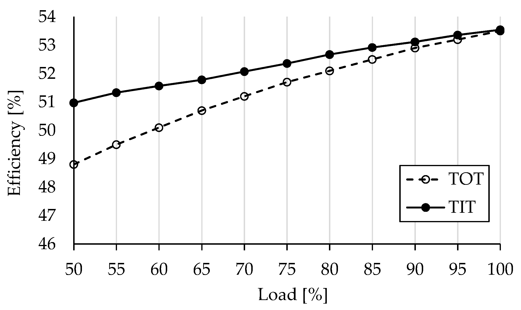
4.2.1. Exergy Efficiency of the Power Plant

As can be seen in Figure 5, the exergy efficiency of the plant decreases during partial load operation with both TIT and TOT control mechanisms. However, with the TIT control, the efficiency decreases less and the power plant is more efficient at low loads. Therefore, for prolonged operation at low capacity factors, TIT control is advised.

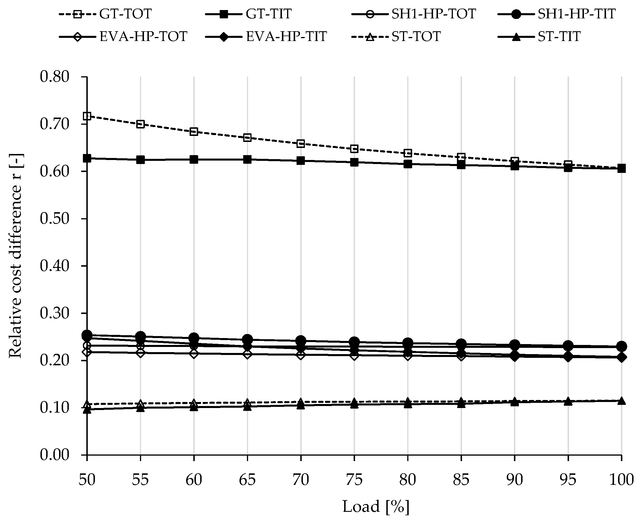
4.2.2. Performance of Individual Components

Figure 6 illustrates the performance of some components with the highest exergoeconomic cost of exergy destruction C ˙ e x , D during the partial load operation of the plant, in terms of Relative cost difference   r , defined according to relation Equation (12),
r = c p c f c f = 1 η e x 1 .
An increase in the Relative cost difference represents an increase of the specific cost of the product of the component, with fixed cost of the fuel—this mirrors a decrease in the efficiency. The results show that, although the TIT control always leads to a globally higher efficiency, some components may individually be more costly. Therefore, improvements may be considered for these components. Specifically, for the gas turbine, the performance is better with TIT at partial load, while the performance of the high pressure evaporator and first high pressure super-heater is worse with TIT control.

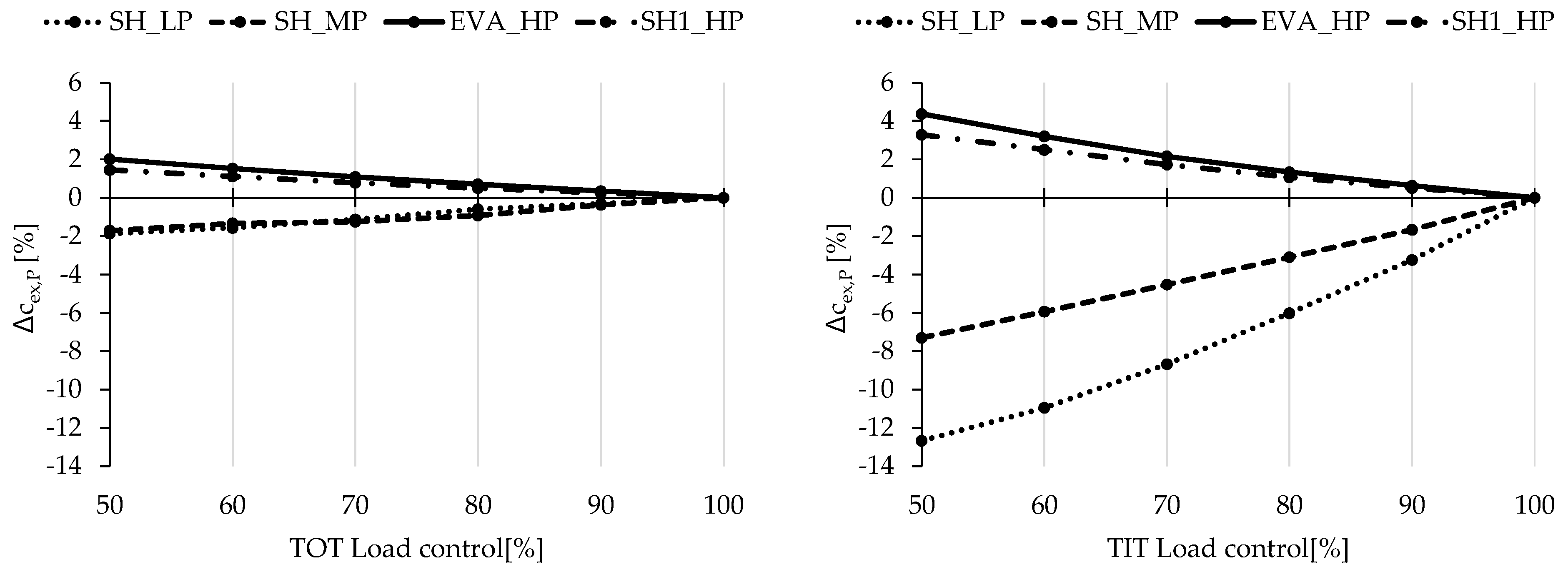
4.2.3. Interrelations among Components

After evaluating the efficiency of the components individually, as a function of the load, the next useful step under the operator’s perspective is to analyze the interrelation between components. Parts of the power plant like the HRSG are almost a black box, where few quantities over few components are monitored. It may happen that a component experiences a failure, but this is not tracked, because the other components counterbalance the failure and the overall performance does not change significantly. In this case, an anomaly has occurred, and the operators are interested in tracking back, although it does not significantly affect the global performance. With the reduced order TIOA model proposed by the Authors, the operators themselves can predict the normal off-design performance of the components and, thus, track possible anomalies without the need of external expertise.
In the present case, the efficiency of the low pressure economizer is reduced by decreasing the overall heat transfer coefficient U, assumed as a proxy for the fouling. This component is chosen since the low temperature heat exchangers are subject to fouling more than others. Figure 7 shows the relative difference of the exergy efficiency of other heat exchangers in the HRSG when the heat transfer coefficient of the ECO-LP is decreased by 10%. The only considerable effect is noticed in the low pressure super-heater, and it is positive. The changes in efficiencies on the other heat exchangers are negligible. The super-heater counterbalances the effects of a reduction in the efficiency of the economizer, and this is due to the reduction in the mass flow rate of steam produced—when the economizer is subject to fouling, the temperature difference between the water and the gases increases, while the pressure and the mass flow rate slightly decrease. The super-heater is sensitive to this decrease, since it elaborates a much lower mass flow rate. Consequently, the temperature difference across it decreases and its efficiency increases. The effect is less intense at lower loads. The fluctuations of the curves are due to a number of interactions between the control mechanisms of all the components in the power plant, but they are limited and do not prevent clear trends to be identified for the low pressure economizer and super-heater. The numerical inaccuracy does not affect these trends, since it is found to be three orders of magnitude smaller than the variations in Figure 7.

4.2.4. Comparison of the Fixed and Functional-Coefficients Approaches

Input–Output models are traditionally adopted to estimate the effects that changes in the final demand would have on the specific and total costs of the system products. Such applications usually rely on the linearity assumption, considering Technical Coefficients as constants [27,38]. This assumption is suited for the analysis of national economies, where the technological level of the productive sectors depends on many processes lumped together, and it is derived from extensive data collection processes [20,39]. However, the linearity assumption may not always accurately represent the behavior of detailed energy systems, since any change in the final demand or operating conditions of such systems may greatly affect the performance of single components.
Figure 8 shows the results of the comparison between the TIOA approach employed in this work (with functional technical coefficients) and the traditional approach based on the linearity assumption (with fixed technical coefficients). The relative deviation between the two approaches has been computed for the unit exergy cost of the product of different heat exchangers ( Δ c e x , P , %), considering both TIT and TOT control mechanisms. With decreasing load and TOT control, the two approaches do not differ significantly. On the contrary, with decreasing load and TIT control, the difference sharply increases, indicating that the linearity assumption is not appropriate for the off-design evaluation of La Casella NGCC.

5. Conclusions

In this paper, a Thermoeconomic Input–Output Analysis (TIOA) model for the on- and off-design performance prediction of energy systems has been proposed, and applied to La Casella NGCC power plant, operating in northern Italy. The TIOA model is stand-alone, in the sense that performance predictions can be performed at every load and with different load control mechanisms, without making further use of the thermodynamic and the economic models. Therefore, they can also be carried out by the power plant operators, who are not into the detailed thermodynamic modeling and need to reduce the complexity of the solution algorithms and the reduced computational effort. The model inherently formalizes the huge amount of information contained in the outputs in an effective way, accounting for the needs of power plant operators.
The model has been applied to an NGCC power plant subject to flexible operation in northern Italy. The on-design evaluation identifies, based on the exergoeconomic costs of exergy destructions, which components should be thermodynamically improved with priority: the GT, ST, EVA-HP, SH1-HP, and the ECO-LP. The off-design evaluation analyzes the performance of the plant at different levels: the global exergy efficiency, the exergy efficiency of individual components, and the interrelation between the exergy efficiency of different components. With the first level evaluation, the TIT control mechanism is identified to better perform at partial loads, than TOT; in the second level, it is shown that, even when the global performance is better, some components may be less efficient (such as the EVA-HP and SH1-HP); the third level evaluation shows that if the ECO-LP is subject to fouling, the SH-LP may counterbalance its decrease in efficiency, preventing the malfunction from being diagnosed. Finally, a comparison between the approach proposed in this paper for off-design evaluation and the reference approach employed in traditional Input–Output economic accounting is presented, in order to highlight the necessity of the first one for this application.
The study provides power plant operators with a tool to predict and to diagnose the off-design performance of power plants undergoing cycling operation. This contributes to abating the informational barriers between scientific research and industrial practice.

Acknowledgments

The authors would like to thank Enel Produzione S.p.A., the Director and the staff of La Casella (PC) power plant for their kind collaboration and support to the realization of this study.

Author Contributions

All the authors equally contributed to this work as follows; Thermoeconomic Input-Output Analysis (TIOA) is the main research field of Sajjad Keshavarzian to predict the off-design behavior, and performing diagnosis of the energy systems. Together with Francesco Gardumi who did his PhD on power plant flexibility and energy systems modelling, the plant has been modeled and validated in Thermoflow Thermoflex™ modeling environment, and the results have been extracted to compute the exergy of all the streams. The Input-Output model has been set; collaborating with Matteo V. Rocco who is working on the industrial ecology and life cycle assessment. Emanuela Colombo supervised the whole work and managed the meetings with the plant’s operators to understand their needs. Furthermore, all the authors contributed in the writing part as well as in the review process of the article.

Conflicts of Interest

The authors declare no conflict of interest.

Abbreviations

The following abbreviations are used in this manuscript:
ECT
Exergy Cost Therory
ECO-LP
Low Pressure Economizer
EVA-HP
High Pressure Evaporator
ExA
Exergy Analysis
GT
Gas Turbine
HRSG
Heat Recovery Steam Generator
IO
Input–Output
IGVs
Inlet Guide Vanes
LCM
Leontief Cost Model
LHV
Lower Heating Value
O&M
Operating and Maintenance
NGCC
Natural Gas Combined Cycle
PECs
Purchased Equipment Costs
RPL
Resource-Product-Losses
ST
Steam Turbine
SH1-HP
First High Pressure Super-Heater
TA
Thermoeconomic Analysis
TIOA
Thermoeconomic Input–Output Analysis
TOT
Turbine Outlet Temperature
TIT
Turbine Inlet Temperature
TRR
Total Revenue Requirement

References

  1. Holz, F.; Richter, P.M.; Egging, R. The Role of Natural Gas in a Low-Carbon Europe: Infrastructure and Regional Supply Security in the Global Gas Model. Available online: https://www.diw.de/documents/publikationen/73/diw_01.c.417156.de/dp1273.pdf (accessed on 20 February 2016).
  2. Prandoni, V.; Rinaldi, C. Documento di sintesi di Progetto “Flessibilità e affidabilità degli impianti a ciclo combinato” Anno 2007. Available online: http://doc.rse-web.it/doc/doc-sfoglia/08000976-589/08000976-589.html (accessed on 20 February 2016). (In Italian)
  3. Kumar, N.; Besuner, P.; Lefton, S.; Agan, D.; Hilleman, D. Power Plant Cycling Costs. Available online: http://www.nrel.gov/docs/fy12osti/55433.pdf (accessed on 22 February 2016).
  4. Garduno-Ramirez, R.; Lee, K.Y. Multiobjective optimal power plant operation through coordinate control with pressure set point scheduling. IEEE Trans. Energy Convers. 2001, 16, 115–122. [Google Scholar] [CrossRef]
  5. Möller, B.F.; Genrup, M.; Assadi, M. On the off-design of a natural gas-fired combined cycle with CO2 capture. Energy 2007, 32, 353–359. [Google Scholar] [CrossRef]
  6. Nord, L.O.; Anantharaman, R.; Bolland, O. Design and off-design analyses of a pre-combustion CO2 capture process in a natural gas combined cycle power plant. Int. J. Greenh. Gas Control 2009, 3, 385–392. [Google Scholar] [CrossRef]
  7. Rovira, A.; Sánchez, C.; Muñoz, M.; Valdés, M.; Durán, M.D. Thermoeconomic optimisation of heat recovery steam generators of combined cycle gas turbine power plants considering off-design operation. Energy Convers. Manag. 2011, 52, 1840–1849. [Google Scholar] [CrossRef]
  8. Rancruel, D.F.; von Spakovsky, M.R. Decomposition with thermoeconomic isolation applied to the optimal synthesis/design and operation of an advanced tactical aircraft system. Energy 2006, 31, 3327–3341. [Google Scholar] [CrossRef]
  9. Campos-Celador, Á.; Pérez-Iribarren, E.; Sala, J.M.; del Portillo-Valdés, L.A. Thermoeconomic analysis of a micro-CHP installation in a tertiary sector building through dynamic simulation. Energy 2012, 45, 228–236. [Google Scholar] [CrossRef]
  10. Peeters, A.N.M.; Faaij, A.P.C.; Turkenburg, W.C. Techno-economic analysis of natural gas combined cycles with post-combustion CO2 absorption, including a detailed evaluation of the development potential. Int. J. Greenh. Gas Control 2007, 1, 396–417. [Google Scholar] [CrossRef]
  11. Verda, V.; Borchiellini, R. Exergy method for the diagnosis of energy systems using measured data. Energy 2007, 32, 490–498. [Google Scholar] [CrossRef]
  12. Kotas, T.J. The Exergy Method of Thermal Plant Analysis; Elsevier: Amsterdam, The Netherlands, 2013. [Google Scholar]
  13. Moran, M.J.; Shapiro, H.N.; Boettner, D.D.; Bailey, M.B. Fundamentals of Engineering Thermodynamics; John Wiley & Sons: New York, NY, USA, 2010. [Google Scholar]
  14. Bejan, A.; Tsatsaronis, G.; Moran, M.J. Thermal Design and Optimization; Wiley: New York, NY, USA, 1996. [Google Scholar]
  15. Verda, V. Prediction of the fuel impact associated with performance degradation in power plants. Energy 2008, 33, 213–223. [Google Scholar] [CrossRef]
  16. Verda, V.; Serra, L.; Valero, A. Thermoeconomic Diagnosis: Zooming Strategy Applied to Highly Complex Energy Systems. Part 1: Detection and Localization of Anomalies*. J. Energy Resour. Technol. 2005, 127, 42–49. [Google Scholar] [CrossRef]
  17. Torres, C.; Valero, A.; Rangel, V.; Zaleta, A. On the cost formation process of the residues. Energy 2008, 33, 144–152. [Google Scholar] [CrossRef]
  18. Erlach, B.; Serra, L.; Valero, A. Structural theory as standard for thermoeconomics. Energy Convers. Manag. 1999, 40, 1627–1649. [Google Scholar] [CrossRef]
  19. Valero, A.; Serra, L.; Uche, J. Fundamentals of exergy cost accounting and thermoeconomics. Part I: Theory. J. Energy Resour. Technol. 2006, 128, 1–8. [Google Scholar] [CrossRef]
  20. Leontief, W.W.; Leontief, W. Input-Output Economics; Oxford University Press: Oxford, UK, 1986. [Google Scholar]
  21. Ameri, M.; Ahmadi, P.; Khanmohammadi, S. Exergy analysis of a 420 MW combined cycle power plant. Int. J. Energy Res. 2008, 32, 175–183. [Google Scholar] [CrossRef]
  22. Querol, E.; González-Regueral, B.; Benedito, J.L.P. Practical Approach to Exergy and Thermoeconomic Analyses of Industrial Processes; Springer: Berlin, Germany, 2012. [Google Scholar]
  23. Valero, A.; Torres, C. Thermoeconomic analysis. In Exergy, Energy System Analysis and Optimization; Encyclopedia of Life Support Systems (EOLSS): Oxford, UK, 2006. [Google Scholar]
  24. Usón, S.; Kostowski, W.J.; Kalina, J. Thermoeconomic Evaluation of Biomass Conversion Systems. In Alternative Energies; Springer: Berlin, Germany, 2013; pp. 69–91. [Google Scholar]
  25. Leontief, W. Input-output analysis. In The New Palgrave: A Dictionary of Economics; Palgrave Macmillan: London, UK, 1987; Volume 2, pp. 860–864. [Google Scholar]
  26. Agudelo, A.; Valero, A.; Torres, C. Allocation of waste cost in thermoeconomic analysis. Energy 2012, 45, 634–643. [Google Scholar] [CrossRef]
  27. Miller, R.E.; Blair, P.D. Input-Output Analysis: Foundations and Extensions; Cambridge University Press: Cambridge, UK, 2009. [Google Scholar]
  28. Querol, E.; Gonzalez-Regueral, B.; Ramos, A.; Perez-Benedito, J.L. Novel application for exergy and thermoeconomic analysis of processes simulated with Aspen Plus. Energy 2011, 36, 964–974. [Google Scholar] [CrossRef] [Green Version]
  29. Rao, A. Sustainable Energy Conversion for Electricity and Coproducts: Principles, Technologies, and Equipment; Wiley: New York, NY, USA, 2015. [Google Scholar]
  30. Loh, H.P.; Lyons, J.; White, C.W.I. Process Equipment Cost Estimation, Final Report; The Office of Scientific and Technical Information: Washington, DC, USA, 2002; pp. 1–78. [Google Scholar]
  31. Thermoflow. Available online: http://www.thermoflow.com/ (accessed on 22 February 2016).
  32. Cafaro, S.; Napoli, L.; Traverso, A.; Massardo, A.F. Monitoring of the thermoeconomic performance in an actual combined cycle power plant bottoming cycle. Energy 2010, 35, 902–910. [Google Scholar] [CrossRef]
  33. Tidball, R.; Bluestein, J.; Rodriguez, N.; Knoke, S. Cost and Performance Assumptions for Modeling Electricity Generation Technologies. Available online: http://www.nrel.gov/docs/fy11osti/48595.pdf (accessed on 22 February 2016).
  34. Updated Capital Cost Estimates for Electricity Generation Plants. Available online: http://www.eia.gov/oiaf/beck_plantcosts/ (accessed on 22 February 2016).
  35. Gestore Mercati Energetici. Available online: http://www.mercatoelettrico.org/en/default.aspx (accessed on 22 February 2016). (In Italian)
  36. Frangopoulos, C.A. Thermo-economic functional analysis and optimization. Energy 1987, 12, 563–571. [Google Scholar] [CrossRef]
  37. Tsatsaronis, G. Thermoeconomic analysis and optimization of energy systems. Prog. Energy Combust. Sci. 1993, 19, 227–257. [Google Scholar] [CrossRef]
  38. Nakamura, S.; Kondo, Y. Waste Input-Output Analysis: Concepts and Application to Industrial Ecology; Springer Science & Business Media: New York, NY, USA, 2009. [Google Scholar]
  39. Diehl, E.W. Adjustment dynamics in a static input–output model. In Proceedings of The 3rd International Conference of the System Dynamics Society, Keystone, CO, USA, July 1985; pp. 161–178.
Figure 1. General outline of the Input–Output tables of a physical system.
Entropy 18 00071 g001
Figure 2. Power plant model and legend of the components.
Entropy 18 00071 g002
Figure 3. T-Q diagram of the HRSG.
Entropy 18 00071 g003
Figure 4. Essential physical structure of the plant.
Entropy 18 00071 g004
Figure 5. Exergy efficiency of the power plant with TIT and TOT control mechanism, as a function of the gas turbine load.
Entropy 18 00071 g005
Figure 6. Relative cost difference of key components, as a function of the gas turbine load.
Entropy 18 00071 g006
Figure 7. Effect of 10% degradation of the heat exchange coefficient of ECO-LP on other components.
Entropy 18 00071 g007
Figure 8. Difference in the unit exergy cost of the product of heat exchangers between the fixed-coefficients approach and the functional coefficients approach.
Entropy 18 00071 g008
Table 1. Inputs for on- and off-design Thermodynamic model.
CategoryVariableUnitsValues
Common inputsEnvironmental TemperatureK288.15
Environmental Pressurebar101.325
Condenser pressurebar0.0336
Cooling water Temperature differenceK6.5
On-design model inputsGas Turbine model and nominal power-Siemens V94.3a, 252 MW
Air mass flow ratekg/s635.9 kg/s
Fuel mass flow ratekg/s14.17 kg/s
HP, MP, LP steam Temperature at turbine inletK813; 813; 618
HP, MP, LP steam Pressure at turbine inletbar88.8; 12.6; 3.3
HP, MP, LP steam turbine nominal efficiency%85; 88; 91
Recirculation ratio at ECO-LP%29
Desired water/steam temperatures at heat exchangers outlet-According to the STs requirement
Mass flow ratios at branching-According to the design layout
Off-design model inputsUA of heat exchangers in HRSGW/KGiven by the on-design computation
Gas turbine load%50–100
Off-design gas turbine control mechanism-TOT or TIT control
Heat transfer coefficient of ECO-LPkW/°C1542; 1388
Table 2. Purchased Equipment Costs (PECs) from the industrial database [30,31].
EquipmentCost [M€]
Gas turbine66.025
Steam turbine32.261
HRSG25.040
Condenser2.442
Pumps0.514
Deareator0.426
Piping0.823
Table 3. Economic parameters for the computation of Total Revenue Requirement (TRR).
ParameterUnitsValue
Year of constructionyear2000
Duration of constructionyears2
Economic lifeyears30
Tax lifeyears15
Inflation rate%2.16
Nominal escalation rate for natural gas%6
Cost of natural gas€/GJ4
Ratio of equity/preferred stock/debt%35/15/50
Return on equity/preferred stock/debt%15/11.7/10
Tax/Property tax/Insurance rate%38/1.5/0.5
Allocation of investment 1st/2nd year%40/60
Table 4. Resource-Product-Losses (RPL) classification.
ComponentsFuel (R)Product (P)Losses (L)
GT2 + 1 + (42 – 43)3 + 46-
DEA39(19 – 18) + 37 + 38-
ST(32 + 34 + 41) – (33 + 35 + 36 + 42)47 + 48 + 49 + 50-
ECO-LP14 – 1518 – 17-
EVA-LP13 – 1439 + (40 – 38)-
SH-LP10 – 1141 – 40-
ECO-MP12 – 13(21 − 20) + (27 – 26)-
EVA-LP11 – 1222 – 21-
SH-MP8 – 923 – 22-
RH1-MP6 – 724 – (23 + 33)-
RH2-MP4 – 534 – (24 + 25)-
ECO2-HP9 – 1028 – 27-
EVA-HP7 – 829 – 28-
SH1-HP5 – 630 – 29-
SH2-HP3 – 432 – (30 + 31)-
LP-P4817 – 16-
MP-P4920 + 25 – 19-
HP-P5026 + 31 – 37-
COND35 + 36 + 43 – 16-45 – 44
Table 5. Results of the Thermoeconomic Input–Output Analysis (TIOA) in the on-design case.
NComponentsExDηexcex,PCex,PCex,Dceco,PCeco,PZCeco,D
MW-J/JMWMW€/GJ€/h€/h€/h
1GT283.30.621.61443.1283.625.725,481.910,744.616,306.1
2DEA0.00.962.4500.0123.9069.44.2
3ST14.70.902.43306.832.160.627,488.55250.02875.8
4ECO_LP3.70.712.4506.556.50524.1540.2
5EVA_LP1.40.832.1302.545.40241.5192.8
6SH_LP0.70.573.0201.256.3021.178.8
7ECO_MP1.40.882.0202.642.00304.1192.0
8EVA_MP2.90.822.1505.143.90385.4374.3
9SH_MP0.80.672.5901.551.1049.9103.2
10RH1_MP3.00.752.3305.244.80194.1362.3
11RH2_MP3.20.822.1505.741.20283.0393.0
12ECO2_HP1.70.872.0303.042.40357.4223.8
13EVA_HP10.10.832.13017.841.801098.71259.2
14SH1_HP5.80.812.17010.341.90530.7714.6
15SH2_HP1.00.822.1401.740.9084.9117.6
16LP P0.40.1516.7901.0480.2015.7105.4
17MP P0.00.673.7700.0126.703.44.3
18HP P0.40.693.6601.1109.7064.5116.2
19COND11.40.1812.16--289.9-397.3-

