A Novel Weak Fuzzy Solution for Fuzzy Linear System

Abstract

This article proposes a novel weak fuzzy solution for the fuzzy linear system. As a matter of fact, we define the right-hand side column of the fuzzy linear system as a piecewise fuzzy function to overcome the related shortcoming, which exists in the previous findings. The strong point of this proposal is that the weak fuzzy solution is always a fuzzy number vector. Two complex and non-complex linear systems under uncertainty are tested to validate the effectiveness and correctness of the presented method.

1. Introduction and Motivation

The system of linear equations plasy a crucial role in the mathematical models of real-world issues such as economic, physics and engineering [1,2,3,4,5]. Due to the uncertain parameters appearing in substantive problems, people often use fuzzy number in a real or complex form to describe fuzzy factors of the complex or real linear system, thus discovering new and easy-implemented schemes that would suitably deal with the fuzzy linear systems (FLS) and solve them, and enabling an expansion to a hotspot exploration [6,7,8,9,10,11,12,13,14,15,16].

One of the pioneer works in this domain was proposed in [17]. In this work, the authors suggested a typical model for solving the $N\times N$ FLS in which the left-hand side matrix assumes to be non-fuzzy and the right-hand side column is an arbitrary fuzzy number. An embedding method [18] is adopted and the original $(n\times n)$ FLS is substituted with the $(2N)\times (2N)$ non-fuzzy linear system. Unfortunately, this was shown to be an incorrect approach in [19]. They showed with a counterexample that the suggested weak fuzzy solution, the Definition 3 in [17], is not always a fuzzy number vector. It is a fact that, in some cases, the solution vector obtained via this method is a non-fuzzy number. However, they have not suggested an alternative definition that could eliminate the aforementioned defect.

In this paper, we revisit the weak fuzzy solution (see Definition 3 in [17]) and propose a variant weak fuzzy solution using a new condition, that is considering the right-hand side column in piecewise form to tackle the limitation found in [19]. Using this new condition, we show analytically (solving the counter example—Example 3.1 in [19]) that the proposed weak fuzzy solution is always a fuzzy number vector. Besides that, to demonstrate the validity of the such approach for the uncertain complex system of linear equations, an example is provided.

The organization of the presentation is as follows. Section 2 revisits the FLS solution. Section 3 describes the proposed method with details. Some conclusions are drawn in Section 4.

2. Fuzzy Linear Systems Revisit

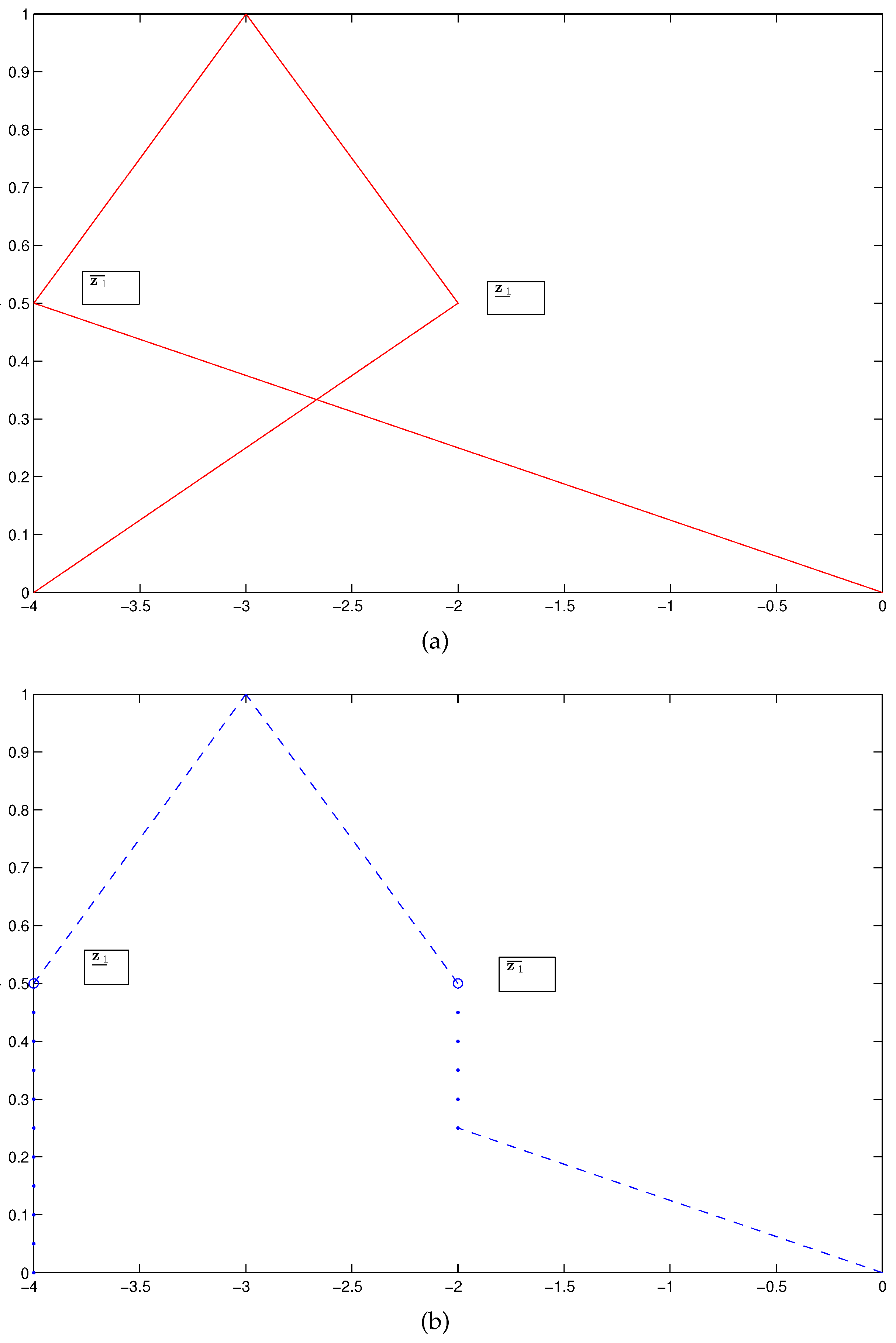
In this section, we briefly explain the Freidman et al. approach [17]. Before that, some preliminaries which are important for this discussion, are recalled. Interested readers are encouraged to read the original paper for more details of fuzzy linear systems and [20] for the fuzzy complex systems.

Definition 1. 

A fuzzy number τ with parametric representation $(\underline{\tau }(\alpha ),\overline{\tau }(\alpha ))$ for all α belongs to $[0,1]$ should fulfill the following conditions:

(a) 

$\underline{\tau }(\alpha )$ is a bounded left-continuous non-decreasing function over $[0,1]$;

(b) 

$\overline{\tau }(\alpha )$ is a bounded right-continuous non-increasing function over $[0,1]$;

(c) 

$\underline{\tau }(\alpha )\le \overline{\tau }(\alpha )$, $0\le \alpha \le 1$.

Definition 2. 

(Fuzzy complex number). A fuzzy complex number can be described as $\tilde{\xi }=r+is$, where $r=[\underline{r}(\alpha ),\overline{r}(\alpha )]$ and $s=[\underline{s}(\alpha ),\overline{s}(\alpha )]$, for all $0\le \alpha \le 1$.

Or it can be written as: $\tilde{\xi }=[\underline{r}(\alpha ),\overline{r}(\alpha )]+i[\underline{s}(\alpha ),\overline{s}(\alpha )]=[\underline{r}(\alpha )+i\underline{s}(\alpha ),\overline{r}(\alpha )+i\overline{s}(\alpha )].$ Now writing $\tilde{\xi }=[\underline{\xi },\overline{\xi }]$, it gives $\underline{\xi }=\underline{r}(\alpha )+i\underline{s}(\alpha )$ and $\overline{\xi }=\overline{r}(\alpha )+i\overline{s}(\alpha ).$

Definition 3. 

(Fuzzy complex arithmetic). Let us assume that ${\tilde{\xi }}_1=[r_1(\alpha ),s_1(\alpha )]$ and ${\tilde{\xi }}_2=[r_2(\alpha ),s_2(\alpha )]$ (where $r_1,s_1,r_2$ and $s_2$ are fuzzy numbers), the fuzzy complex arithmetic is written for addition and multiplication as

(a) 

${\tilde{\xi }}_1+{\tilde{\xi }}_2=(r_1+r_2)+i(s_1+s_2),$

(b) 

${\tilde{\xi }}_1\times {\tilde{\xi }}_2=\{(r_1\times r_2)-(s_1\times s_2)\}+i\{(r_1\times s_2)+(s_1\times r_2)\}.$

Definition 4. 

The $N\times N$ linear system:

$$\left\{\begin{array}{c}{\theta }_{11}{\mathbf{z}}_1+{\theta }_{12}{\mathbf{z}}_2+\cdots +{\theta }_{1n}{\mathbf{z}}_n={\psi }_1,\\ {\theta }_{21}{\mathbf{z}}_1+{\theta }_{22}{\mathbf{z}}_2+\cdots +{\theta }_{2n}{\mathbf{z}}_n={\psi }_2,\\ ⋮\\ {\theta }_{n1}{\mathbf{z}}_1+{\theta }_{n2}{\mathbf{z}}_2+\cdots +{\theta }_{nn}{\mathbf{z}}_n={\psi }_n.\end{array}\right.$$

(1)

In Equation (1) the matrix of coefficients, $\Theta =({\theta }_{ij})$, for $1\le i,j\le N$, is a non-fuzzy $N\times N$ matrix, and ${\psi }_{i\in \{1,2,\cdots ,N\}}$ are fuzzy numbers is named the FLS. Using the embedding approach [18], the system of Equation (1) is converted to the subsequent $2N\times 2N$ deterministic linear system:

$$\Lambda \mathbf{Z}=\Psi ,\Rightarrow \left[\begin{array}{cc}{\Lambda }_1\ge 0& {\Lambda }_2\le 0\\ {\Lambda }_2\ge 0& {\Lambda }_1\ge 0\end{array}\right]\left[\begin{array}{c}\underline{\mathbf{Z}}\\ -\overline{\mathbf{Z}}\end{array}\right]=\left[\begin{array}{c}\underline{\Psi }\\ -\overline{\Psi }\end{array}\right],$$

(2)

in which

$$\begin{array}{c}\mathbf{Z}={({\underline{\mathbf{z}}}_1,{\underline{\mathbf{z}}}_2,...,{\underline{\mathbf{z}}}_n,-{\overline{\mathbf{z}}}_1,-{\overline{\mathbf{z}}}_2,...,-{\overline{\mathbf{z}}}_n)}^T\hfill \end{array},$$

$$\begin{array}{c}\Psi ={({\underline{\psi }}_1,{\underline{\psi }}_2,...,{\underline{\psi }}_n,-{\overline{\psi }}_1,-{\overline{\psi }}_2,...,-{\overline{\psi }}_n)}^T\hfill \end{array},$$

and ${\lambda }_{ij}\in \{{\Lambda }_1.\Lambda 2\}$ in Equation (2) are specified as follows:

$$\left\{\begin{array}{c}{\lambda }_{ij}={\theta }_{ij},{\lambda }_{i+n,j+n}={\theta }_{ij},if{\theta }_{ij}\ge 0\\ {\lambda }_{i,j+n}=-{\theta }_{ij},{\lambda }_{i+n,j}=-{\theta }_{ij},if{\theta }_{ij}<0\end{array}\right.$$

and for the other not stated values, ${\lambda }_{ij}$ is zero [17].

Definition 5. 

Let $\mathbf{Z}=\left\{({\underline{\mathbf{z}}}_i,{\overline{\mathbf{z}}}_i)|i=1,2,...,N\right\}$ is the unique solution of the $(2N)\times (2N)$ non-fuzzy linear system (2). The fuzzy number vector $\mathfrak{D}=\left\{({\underline{d}}_i,{\overline{d}}_i)|i=1,2,...,n\right\}$ defined by

$$\begin{array}{c}{\underline{d}}_i(\alpha )=\underset{0\le \alpha \le 1}{min}\left\{{\underline{\mathbf{z}}}_i(\alpha ),{\overline{\mathbf{z}}}_i(\alpha ),{\underline{\mathbf{z}}}_i(1)\right\},\hfill \end{array}$$

(3)

$$\begin{array}{c}{\overline{d}}_i(\alpha )=\underset{0\le \alpha \le 1}{max}\left\{{\underline{\mathbf{z}}}_i(\alpha ),{\overline{\mathbf{z}}}_i(\alpha ),{\underline{\mathbf{z}}}_i(1)\right\},\hfill \end{array}$$

(4)

is the fuzzy solution of $\Lambda \mathbf{Z}=\Psi$. If $({\underline{\mathbf{z}}}_i,{\overline{\mathbf{z}}}_i)$ where $i=1,2,\cdots ,N$ are all fuzzy numbers, ${\underline{d}}_i={\underline{\mathbf{z}}}_i$ and ${\overline{d}}_i={\overline{\mathbf{z}}}_i$, $\mathfrak{D}$ is a strong fuzzy solution; else $\mathfrak{D}$ is a weak fuzzy solution.

However, Allahviranloo et al. [19] showed with a counterexample, which we will detail in Example 1, that the weak fuzzy solutions proposed by Freidman et al. [17] are not fuzzy number vectors in general. Indeed, they employed the definition for weak fuzzy solution, introduced in [21], where Equations (3) and (4) are transformed to the following:

$$\begin{array}{c}{\underline{d}}_i(\alpha )=\underset{0\le \alpha \le 1}{min}\left\{{\underline{\mathbf{z}}}_i(\alpha ),{\overline{\mathbf{z}}}_i(\alpha ),{\underline{\mathbf{z}}}_i(1),{\overline{\mathbf{z}}}_i(1)\right\},\hfill \end{array}$$

(5)

$$\begin{array}{c}{\overline{d}}_i(\alpha )=\underset{0\le \alpha \le 1}{max}\left\{{\underline{\mathbf{z}}}_i(\alpha ),{\overline{\mathbf{z}}}_i(\alpha ),{\underline{\mathbf{z}}}_i(1),{\overline{\mathbf{z}}}_i(1)\right\}.\hfill \end{array}$$

(6)

Example 1. 

[Example 3.1 in [19]]. Consider the following $2\times 2$ FLS

$$\left\{\begin{array}{c}{\mathbf{z}}_1+{\mathbf{z}}_2=({\underline{\psi }}_1(\alpha ),{\overline{\psi }}_1(\alpha ))\\ {\mathbf{z}}_1+2{\mathbf{z}}_2=({\underline{\psi }}_2(\alpha ),{\overline{\psi }}_2(\alpha ))\end{array},\right.$$

(7)

where

$${\underline{\psi }}_1(\alpha )=\left\{\begin{array}{c}8\alpha -14,0\le \alpha \le \frac{1}{2}\\ 2\alpha -11,\frac{1}{2}\le \alpha \le 1\end{array},\right.$$

$${\overline{\psi }}_1(\alpha )=\left\{\begin{array}{c}-1-13\alpha ,0\le \alpha \le \frac{1}{2}\\ -6-3\alpha ,\frac{1}{2}\le \alpha \le 1\end{array},\right.$$

and

$${\underline{\psi }}_2(\alpha )=\left\{\begin{array}{c}12\alpha -24,0\le \alpha \le \frac{1}{2}\\ 6\alpha -21,\frac{1}{2}\le \alpha \le 1\end{array},\right.$$

$${\overline{\psi }}_2(\alpha )=\left\{\begin{array}{c}-2-18\alpha ,0\le \alpha \le \frac{1}{2}\\ -7-8\alpha ,\frac{1}{2}\le \alpha \le 1\end{array}.\right.$$

By solving this problem, the solution is obtained as follows:

$${\underline{\mathbf{z}}}_1(\alpha )=\left\{\begin{array}{c}4\alpha -4,0\le \alpha \le \frac{1}{2}\\ -2\alpha -1,\frac{1}{2}\le \alpha \le 1\end{array},\right.$$

$${\overline{\mathbf{z}}}_1(\alpha )=\left\{\begin{array}{c}-8\alpha ,0\le \alpha \le \frac{1}{2}\\ 2\alpha -5,\frac{1}{2}\le \alpha \le 1\end{array}.\right.$$

and ${\underline{\mathbf{z}}}_2(\alpha )=4\alpha -10$, ${\overline{\mathbf{z}}}_2(\alpha )=-1-5\alpha$. It is clear to verify that ${\mathbf{z}}_2$ is a fuzzy number, but ${\mathbf{z}}_1$ is not a fuzzy number. This is because the conditions in Definition 1 do not hold since, ${\overline{\mathbf{z}}}_1<{\underline{\mathbf{z}}}_1$ for all $r\in (\frac{1}{3},1]$, therefore ${\underline{\mathbf{z}}}_1$ and ${\overline{\mathbf{z}}}_1$ are not non-decreasing nor non-increasing over $[\frac{1}{2},1]$ (see Figure 1).

Using Equation (5) and (6), Allahviranloo et al. [19] showed the following weak fuzzy solution:

$${\underline{d}}_1(\alpha )=\left\{\begin{array}{c}4\alpha -4,0\le \alpha \le \frac{1}{4}\\ -3,\frac{1}{4}\le \alpha \le \frac{3}{8}\\ -8\alpha ,\frac{3}{8}\le \alpha \le \frac{1}{2}\\ 2\alpha -5,\frac{1}{2}\le \alpha \le 1\end{array},\right.$$

$${\overline{d}}_1(\alpha )=\left\{\begin{array}{c}-8\alpha ,0\le \alpha \le \frac{1}{3}\\ 4\alpha -4,\frac{1}{3}\le \alpha \le \frac{1}{2}\\ -2\alpha -1,\frac{1}{2}\le \alpha \le 1\end{array},\right.$$

is not a fuzzy number using the proposal in [17] . In fact, ${\underline{d}}_1(\alpha )$ is not non-decreasing over $[\frac{3}{8},\frac{1}{2}]$, and ${\overline{d}}_1(\alpha )$ is not non-increasing over $[\frac{1}{3},\frac{1}{2}]$.

3. A New Definition for the Weak Fuzzy Solution

Fuzzy solution is some real responses to the engineering problems. In fact, in each level set, we have some intervals included the pessimistic/optimistic solutions which should be converged to the core (as deterministic case). In this regard, we need some fuzzy solutions to interpret the solutions of fuzzy systems correctly. In this section, we describe our proposed weak fuzzy solution with a modification on the Definition 5 due to achieve a accurate weak fuzzy solution for the FLS.

Firstly, we rewrite the $N\times N$ FLS (1) in terms of piecewise right-hand side column as follows:

$$\left\{\begin{array}{c}{\theta }_{11}{\mathbf{z}}_1+{\theta }_{12}{\mathbf{z}}_2+\cdots +{\theta }_{1n}{\mathbf{z}}_n={\psi }_1,\\ {\theta }_{21}{\mathbf{z}}_1+{\theta }_{22}{\mathbf{z}}_2+\cdots +{\theta }_{2n}{\mathbf{z}}_n={\psi }_2,\\ ⋮\\ {\theta }_{n1}{\mathbf{z}}_1+{\theta }_{n2}{\mathbf{z}}_2+\cdots +{\theta }_{nn}{\mathbf{z}}_n={\psi }_n.\end{array}\right.$$

(8)

where

$${\psi }_i(\alpha )=\left\{\begin{array}{c}{\psi }_{i,1}(\alpha ),0\le \alpha \le s_1\\ {\psi }_{i,2}(\alpha ),s_1\le \alpha \le s_2\\ ⋮\\ {\psi }_{i,n+1}(\alpha ),s_n\le \alpha \le 1\end{array},\right.$$

is a piecewise fuzzy number (it is fuzzy number over each subinterval $[s_j,s_{j+1}]$ where $j=0,\cdots ,N$; $s_0=0$; $s_{N+1}=1$). The solution of system (8) will be in piecewise form as follows:

$${\mathbf{z}}_i(\alpha )=\left\{\begin{array}{c}{\mathbf{z}}_{i,1}(\alpha ),0\le \alpha \le s_1\\ {\mathbf{z}}_{i,2}(\alpha ),s_1\le \alpha \le s_2\\ ⋮\\ {\mathbf{z}}_{i,n+1}(\alpha ),s_n\le \alpha \le 1\end{array}.\right.$$

Definition 6. 

Let $\mathbf{X}=\left\{(\underline{{\mathbf{z}}_i},{\overline{\mathbf{z}}}_i)|i=1,2,\cdots ,N\right\}$ is the unique solution of a linear system (2). The fuzzy number vector $\upsilon =({\upsilon }_i)$, such that

$${\upsilon }_i(\alpha )=\left\{({\underline{\upsilon }}_{i,j}(\alpha ),{\overline{\upsilon }}_{i,j}(\alpha ))|i=1,2,\cdots ,N,\right\},$$

(9)

$$\mathit{for}j\in \{1,2,\cdots ,N\}$$

defined by

$$\begin{array}{c}{\underline{\upsilon }}_{i,j}(\alpha )=\underset{s_{j-1}\le \alpha \le s_j}{min}\left\{{\underline{\mathbf{z}}}_{i,j}(\alpha ),{\overline{\mathbf{z}}}_{i,j}(\alpha ),{\underline{\mathbf{z}}}_{i,j}(s_j),{\overline{\mathbf{z}}}_{i,j}(s_j)\right\},\hfill \end{array}$$

(10)

$$\begin{array}{c}{\overline{\upsilon }}_{i,j}(\alpha )=\underset{s_{j-1}\le \alpha \le s_j}{max}\left\{{\underline{\mathbf{z}}}_{i,j}(\alpha ),{\overline{\mathbf{z}}}_{i,j}(\alpha ),{\underline{\mathbf{z}}}_{i,j}(s_j),{\overline{\mathbf{z}}}_{i,j}(s_j)\right\},\hfill \end{array}$$

(11)

where ${\mathbf{z}}_{i,j}(\alpha )=({\underline{\mathbf{z}}}_{i,j}(\alpha ),{\overline{\mathbf{z}}}_{i,j}(r))$ is the i-th solution of system (8) over interval $\alpha \in [s_{j-1},s_j]$ is called the fuzzy solution. If ${\underline{\upsilon }}_{i,j}(\alpha )={\underline{\mathbf{z}}}_{i,j}(\alpha )$ and ${\overline{\upsilon }}_{i,j}(\alpha )={\overline{\mathbf{z}}}_{i,j}(\alpha )$, $\upsilon ={({\upsilon }_j)}_{j=1}^N$ is a strong fuzzy solution, else υ is a weak fuzzy solution.

Employing this new definition of the weak fuzzy solution, we showed through Example 1 that our proposed weak fuzzy solution is always a fuzzy number vector. In fact, using the proposed notations,

$${\mathbf{z}}_1(\alpha )=\left\{\begin{array}{c}{\mathbf{z}}_{1,1}(\alpha ),0\le \alpha \le \frac{1}{2}\\ {\mathbf{z}}_{1,2}(\alpha ),\frac{1}{2}\le \alpha \le 1\end{array},\right.$$

(12)

where ${\mathbf{z}}_{1,1}(\alpha )=(4\alpha -4,-8\alpha )$ and ${\mathbf{z}}_{1,2}(\alpha )=(-2\alpha -1,2\alpha -5)$. Since, it has been proven beforehand that ${\mathbf{z}}_2$ is a fuzzy number, we only focus on the ${\mathbf{z}}_1$. Employing the proposed Definition 6, we have:

$$\begin{array}{cc}{\underline{\upsilon }}_{1,1}(\alpha )\hfill & =\underset{0\le \alpha \le \frac{1}{2}}{min}\left\{{\underline{\mathbf{z}}}_{1,1}(\alpha ),{\overline{\mathbf{z}}}_{1,1}(\alpha ),{\underline{\mathbf{z}}}_{1,1}(\frac{1}{2}),{\overline{\mathbf{z}}}_{1,1}(\frac{1}{2})\right\}\hfill \\ & =-4,\hfill \end{array}$$

$$\begin{array}{cc}{\overline{\upsilon }}_{1,1}(\alpha )\hfill & =\underset{0\le \alpha \le \frac{1}{2}}{max}\left\{{\underline{\mathbf{z}}}_{1,1}(\alpha ),{\overline{\mathbf{z}}}_{1,1}(\alpha ),{\underline{\mathbf{z}}}_{1,1}(\frac{1}{2}),{\overline{\mathbf{z}}}_{1,1}(\frac{1}{2})\right\}\hfill \\ & =\left\{\begin{array}{c}-8\alpha ,0\le \alpha \le \frac{1}{4}\\ -2,\frac{1}{4}\le \alpha \le \frac{1}{2}\end{array}\right.\hfill \end{array},$$

and

$$\begin{array}{cc}{\underline{\upsilon }}_{1,2}(\alpha )\hfill & =\underset{\frac{1}{2}\le \alpha \le 1}{min}\left\{{\underline{\mathbf{z}}}_{1,2}(\alpha ),{\overline{\mathbf{z}}}_{1,2}(\alpha ),{\underline{\mathbf{z}}}_{1,2}(1),{\overline{\mathbf{z}}}_{1,1}(1)\right\}\hfill \\ & =2\alpha -5,\hfill \end{array}$$

(13)

$$\begin{array}{cc}{\overline{\upsilon }}_{1,2}(\alpha )\hfill & =\underset{\frac{1}{2}\le \alpha \le 1}{max}\left\{{\underline{\mathbf{z}}}_{1,2}(\alpha ),{\overline{\mathbf{z}}}_{1,2}(\alpha ),{\underline{\mathbf{z}}}_{1,2}(1),{\overline{\mathbf{z}}}_{1,1}(1)\right\}\hfill \\ & =-2\alpha -1.\hfill \end{array}$$

(14)

Hence, we acquire the weak fuzzy solution ${\mathbf{z}}_1$ as follows:

$${\mathbf{z}}_1(\alpha )=\left\{\begin{array}{c}(-4,-8\alpha ),0\le \alpha \le \frac{1}{4}\\ (-4,-2),\frac{1}{4}\le \alpha \le \frac{1}{2}\\ (2\alpha -5,-2\alpha -1),\frac{1}{2}\le \alpha \le 1\end{array}.\right.$$

From here, it is clearly that ${\mathbf{z}}_1$ is a fuzzy number over $[0,1]$ (see Figure 1b).

Example 2. 

Consider the following complex fuzzy system

$$\left\{\begin{array}{c}{\mathbf{z}}_1+{\mathbf{z}}_2=({\underline{\psi }}_1(\alpha ),{\overline{\psi }}_1(\alpha ))+i({\underline{\zeta }}_1(\alpha ),{\overline{\zeta }}_1(\alpha ))\\ {\mathbf{z}}_1+2{\mathbf{z}}_2=({\underline{\psi }}_2(\alpha ),{\overline{\psi }}_2(\alpha ))+i({\underline{\zeta }}_2(\alpha ),{\overline{\zeta }}_2(\alpha ))\end{array},\right.$$

(15)

where

$${\underline{\psi }}_1(\alpha )={\underline{\zeta }}_1(\alpha )=\left\{\begin{array}{c}8\alpha -14,0\le \alpha \le \frac{1}{2}\\ 2\alpha -11,\frac{1}{2}\le \alpha \le 1\end{array},\right.$$

$${\overline{\psi }}_1(\alpha )={\overline{\zeta }}_1(\alpha )=\left\{\begin{array}{c}-1-13\alpha ,0\le \alpha \le \frac{1}{2}\\ -6-3\alpha ,\frac{1}{2}\le \alpha \le 1\end{array},\right.$$

and

$${\underline{\psi }}_2(\alpha )={\underline{\zeta }}_2(\alpha )=\left\{\begin{array}{c}12\alpha -24,0\le \alpha \le \frac{1}{2}\\ 6\alpha -21,\frac{1}{2}\le \alpha \le 1\end{array},\right.$$

$${\overline{\psi }}_2(\alpha )={\overline{\zeta }}_2(\alpha )=\left\{\begin{array}{c}-2-18\alpha ,0\le \alpha \le \frac{1}{2}\\ -7-8\alpha ,\frac{1}{2}\le \alpha \le 1\end{array},\right.$$

where ${\mathbf{z}}_1={\mathbf{z}}_{11}+i{\mathbf{z}}_{12}$ and ${\mathbf{z}}_2={\mathbf{z}}_{21}+i{\mathbf{z}}_{22}$ are fuzzy complex numbers.

In order to solve this system using Friedman et al. method [17], we should solve two following systems:

$$\left\{\begin{array}{c}{\mathbf{z}}_{11}+{\mathbf{z}}_{21}=({\underline{\psi }}_1(\alpha ),{\overline{\psi }}_1(\alpha ))\\ {\mathbf{z}}_{11}+2{\mathbf{z}}_{21}=({\underline{\psi }}_2(\alpha ),{\overline{\psi }}_2(\alpha ))\end{array},\right.$$

(16)

and

$$\left\{\begin{array}{c}{\mathbf{z}}_{12}+{\mathbf{z}}_{22}=({\underline{\zeta }}_1(\alpha ),{\overline{\zeta }}_1(\alpha ))\\ {\mathbf{z}}_{12}+2{\mathbf{z}}_{22}=({\underline{\zeta }}_2(\alpha ),{\overline{\zeta }}_2(\alpha ))\end{array},\right.$$

(17)

by solving the above systems (implementing the weak solution proposed by Friedman et al. [17]), the following solutions have been obtained:

$${\underline{\mathbf{z}}}_{11}(\alpha )={\underline{\mathbf{z}}}_{12}(\alpha )=\left\{\begin{array}{c}4\alpha -4,0\le \alpha \le \frac{1}{4}\\ -3,\frac{1}{4}\le \alpha \le \frac{3}{8}\\ -8\alpha ,\frac{3}{8}\le \alpha \le \frac{1}{2}\\ 2\alpha -5,\frac{1}{2}\le \alpha \le 1\end{array},\right.$$

$${\overline{\mathbf{z}}}_{11}(\alpha )={\overline{\mathbf{z}}}_{12}(\alpha )=\left\{\begin{array}{c}-8\alpha ,0\le \alpha \le \frac{1}{3}\\ 4\alpha -4,\frac{1}{3}\le \alpha \le \frac{1}{2}\\ -2\alpha -1,\frac{1}{2}\le \alpha \le 1\end{array},\right.$$

and

$${\underline{\mathbf{z}}}_{21}(\alpha )={\underline{\mathbf{z}}}_{22}(\alpha )=4\alpha -10,{\overline{\mathbf{z}}}_{21}(\alpha )={\overline{\mathbf{z}}}_{22}(\alpha )=-1-5\alpha .$$

Clearly, ${\mathbf{z}}_{21}({\mathbf{z}}_{21})$ is fuzzy number, but ${\mathbf{z}}_{11}({\mathbf{z}}_{12})$ is not fuzzy number, even by applying the proposed weak solution.

Now, using the proposed weak solution, we obtain the following solution:

$${\underline{\mathbf{z}}}_{11}(\alpha )=\left\{\begin{array}{c}-4,0\le \alpha \le \frac{1}{4}\\ -4,\frac{1}{4}\le \alpha \le \frac{1}{2}\\ 2-5\alpha ,\frac{1}{2}\le \alpha \le 1\end{array},\right.$$

$${\overline{\mathbf{z}}}_{11}(\alpha )=\left\{\begin{array}{c}-8\alpha ,0\le \alpha \le \frac{1}{4}\\ -2,\frac{1}{4}\le \alpha \le \frac{1}{2}\\ -2\alpha -1,\frac{1}{2}\le \alpha \le 1\end{array}.\right.$$

These results are also valid for ${\mathbf{z}}_{12}.$

4. Conclusion

This study recommended an innovative weak fuzzy solution of FLS that will always be a fuzzy number vector. In particular, we introduce a new definition based on the piecewise right-hand side column. We validated the proposed solution through the counterexample given in [19] and fuzzy complex linear systems.

We aimed to introduce some approaches to represent the solutions as fuzzy numbers. Actually, we did not propose a method to solve the system, we just proposed a method to modify the previously reported fuzzy weak solution which was not a fuzzy number for some cases.

In future works, we will solve some other types of fuzzy systems, for example fuzzy differential equations, fuzzy linear and non linear optimization problems with crisp and fuzzy coefficients, and so on, then we will apply our novel fuzzy weak solutions to state the ability of this modification. Also, we will obtain the error estimation of this interpretation.

References

1. Dimov, I.; Maire, S.; Sellier, J.M. A new Walk on Equations Monte Carlo method for solving systems of linear algebraic equations. Appl. Math. Model. 2015, 39, 4494–4510. [Google Scholar] [CrossRef]
2. Fuyong, L. The solution of linear systems equations with circulant-like coefficient matrices. Appl. Math. Comput. 2013, 219, 8259–8268. [Google Scholar] [CrossRef]
3. Mazandarani, M.; Najariyan, M. A note on “A class of linear differential dynamical systems with fuzzy initial condition”. Fuzzy Sets Syst. 2015, 265, 121–126. [Google Scholar] [CrossRef]
4. Liang, X.S. Entropy evolution and uncertainty estimation with dynamical systems. Entropy 2014, 16, 3605–3634. [Google Scholar] [CrossRef]
5. Chavanis, P.-H. Generalized Stochastic Fokker–Planck Equations. Entropy 2015, 17, 3205–3252. [Google Scholar] [CrossRef]
6. Lodwick, W.A.; Dubois, D. Interval linear systems as a necessary step in fuzzy linear systems. Fuzzy Sets Syst. 2015, 281, 227–251. [Google Scholar] [CrossRef] [Green Version]
7. Otadi, M.A.; Mosleh, M. Simulation and evaluation of dual fully fuzzy linear systems by fuzzy neural network. Appl. Math. Model. 2011, 35, 5026–5039. [Google Scholar] [CrossRef]
8. Allahviranloo, T.; Lotfi, F.H.; Kiasari, M.K.; Khezerloo, M. On the fuzzy solution of LR fuzzy linear systems. Appl. Math. Model. 2013, 37, 1170–1176. [Google Scholar] [CrossRef]
9. Allahviranloo, T.; Ghanbari, M. On the algebraic solution of fuzzy linear systems based on interval theory. Appl. Math. Model. 2012, 36, 5360–5379. [Google Scholar] [CrossRef]
10. Behera, D.; Chakraverty, S. Solving fuzzy complex system of linear equations. Inf. Sci. 2014, 277, 154–162. [Google Scholar] [CrossRef]
11. Amirfakhrian, M. Numerical solution of a fuzzy system of linear equations with polynomial parametric form. Int. J. Comput. Math. 2007, 84, 1089–1097. [Google Scholar] [CrossRef]
12. Sun, X.-D.; Guo, S.-Z. Linear Formed General Fuzzy Linear Systems. Syst. Eng. Theory Pract. 2009, 29, 92–98. [Google Scholar] [CrossRef]
13. Ghanbari, R. Solutions of fuzzy LR algebraic linear systems using linear programs. Appl. Math. Model. 2015, 39, 5164–5173. [Google Scholar] [CrossRef]
14. Nuraei, R.; Allahviranloo, T.; Ghanbari, M. Finding an inner estimation of the solution set of a fuzzy linear system. Appl. Math. Model. 2013, 37, 5148–5161. [Google Scholar] [CrossRef]
15. Muzzioli, S.; Reynaerts, H. Fuzzy linear systems of the form A1x + b1 = A2x + b2. Fuzzy Sets Syst. 2006, 157, 939–951. [Google Scholar] [CrossRef]
16. Shary, S.P. New characterizations for the solution set to interval linear systems of equations. Appl. Math. Comput. 2015, 265, 570–573. [Google Scholar] [CrossRef]
17. Friedman, M.; Ming, M.; Kandel, A. Fuzzy linear systems. Fuzzy Sets Syst. 1998, 96, 201–209. [Google Scholar] [CrossRef]
18. Wu, C.-X.; Ma, M. Embedding problem of fuzzy number space: Part I. Fuzzy Sets Syst. 1991, 44, 33–38. [Google Scholar]
19. Allahviranloo, T.; Ghanbari, M.; Hosseinzadeh, A.A.; Haghi, E.; Nuraei, R. A note on “Fuzzy linear systems”. Fuzzy Sets Syst. 2011, 177, 87–92. [Google Scholar] [CrossRef]
20. Behera, D.; Chakraverty, S. Solving fuzzy complex system of linear equations. Inf. Sci. 2014, 277, 154–162. [Google Scholar] [CrossRef]
21. Zheng, B.; Wang, K. General fuzzy linear systems. Appl. Math. Comput. 2006, 181, 1276–1286. [Google Scholar] [CrossRef]
Figure 1. A comparison between our proposed solution with the solution in [17]. It can be noticed, and was proved in [19] that (a) the solution in [17] is not a fuzzy vector; while using our new definition (Definition 6), (b) the obtained solution is a fuzzy vector. (y-axis represents the α-cuts and x-axis is for the value of fuzzy solution ( z 1 )).
Entropy 18 00068 g001