1. Introduction
In information theory, the relations between entropy and error probability are one of the important fundamentals. Among the related studies, one milestone is Fano’s inequality (also known as Fano’s lower bound for the error probability of decoders), which was originally proposed in 1952 by Fano but formally published in 1961 [
1]. It is well known that Fano’s inequality plays a critical role in deriving other theorems and criteria in information theory [
2,
3,
4]. However, within the research community, it has not been widely accepted exactly who was first to develop the upper bound for the error probability [
5]. According to [
6,
7], Kovalevskij [
8] was recognized as the first to derive the upper bound of the error probability in relation to entropy in 1965. Later, several researchers, such as Chu and Chueh in 1966 [
9], Tebbe and Dwyer in 1968 [
10], Hellman and Raviv in 1970 [
11], independently developed upper bounds.
The lower and upper bounds of error probability have been a long-standing topic in studies on information theory [
6,
7,
12,
13,
14,
15,
16,
17,
18,
19,
20,
21]. However, we consider two issues that have received less attention in these studies:
What are the closed-form relations between each bound and error components in a diagram of entropy and error probability?
What are the lower and upper bounds in terms of the non-Bayesian errors if a non-Bayesian rule is applied in the information processing?
The first issue implies a need for a complete set of interpretations to the bounds in relation to joint distributions, so that both error probability and its error components are known for a deeper understanding. We will discuss the reasons of the need in the later sections of this paper. Up to now, most existing studies derived the bounds through an inequality means without using joint distribution information. Therefore, their bounds are not described by a generic relation to joint distributions so that their error component information cannot be gained. Several significant studies have achieved Fano’s bound from the joint distributions but through different means [
16,
20,
21]. They all did not show the explicit relations to error components. Regarding the second issue, to the best of our knowledge, it seems that no study is shown in open literature on the bounds in terms of the non-Bayesian errors. We will define the Bayesian and non-Bayesian errors in
Section 3. The non-Bayesian errors are also of importance because most classifications are realized within this category.
The issues above form the motivation behind this work. We take binary classifications as a problem background since it is more common and understandable from our daily-life experiences. Moreover, we intend to simplify settings within a binary state and Shannon entropy definitions for a case study from an expectation that the central principle of the approach is well highlighted by simple examples. The novel contribution of the present work is given from the following three aspects:
A new approach is proposed for deriving bounds directly through the optimization process based on a joint distribution, which is significantly different from all other existing approaches. One advantage of using the approach is the closed-form expressions to the bounds and their error components.
A new upper bound in a diagram of “Error Probability vs. Conditional Entropy” for the Bayesian errors is derived with a closed-form expression in the binary state, which has not been reported before. The new bound is generally tighter than Kovalevskij’s upper bound. Fano’s lower bound receives novel interpretations.
The comparison study on the bounds in terms of the Bayesian and non-Bayesian errors are made in the binary state. The bounds of non-Bayesian errors are explored for a first time in information theory and imply a significant role in the study of machine learning and classification applications.
In the first aspect, we also conduct the actual derivation using a symbolic software tool, which presents a standard and comprehensive solution in the approach. The rest of this paper is organized as follows. In
Section 2, we present related works on the bounds. For a problem background of binary classifications, several related definitions are given in
Section 3. The bounds are given and discussed for the Bayesian and non-Bayesian errors in
Section 4 and
Section 5, respectively. Interpretations to some key points are presented in
Section 6. We summarize the work in
Section 7 and present some discussions in
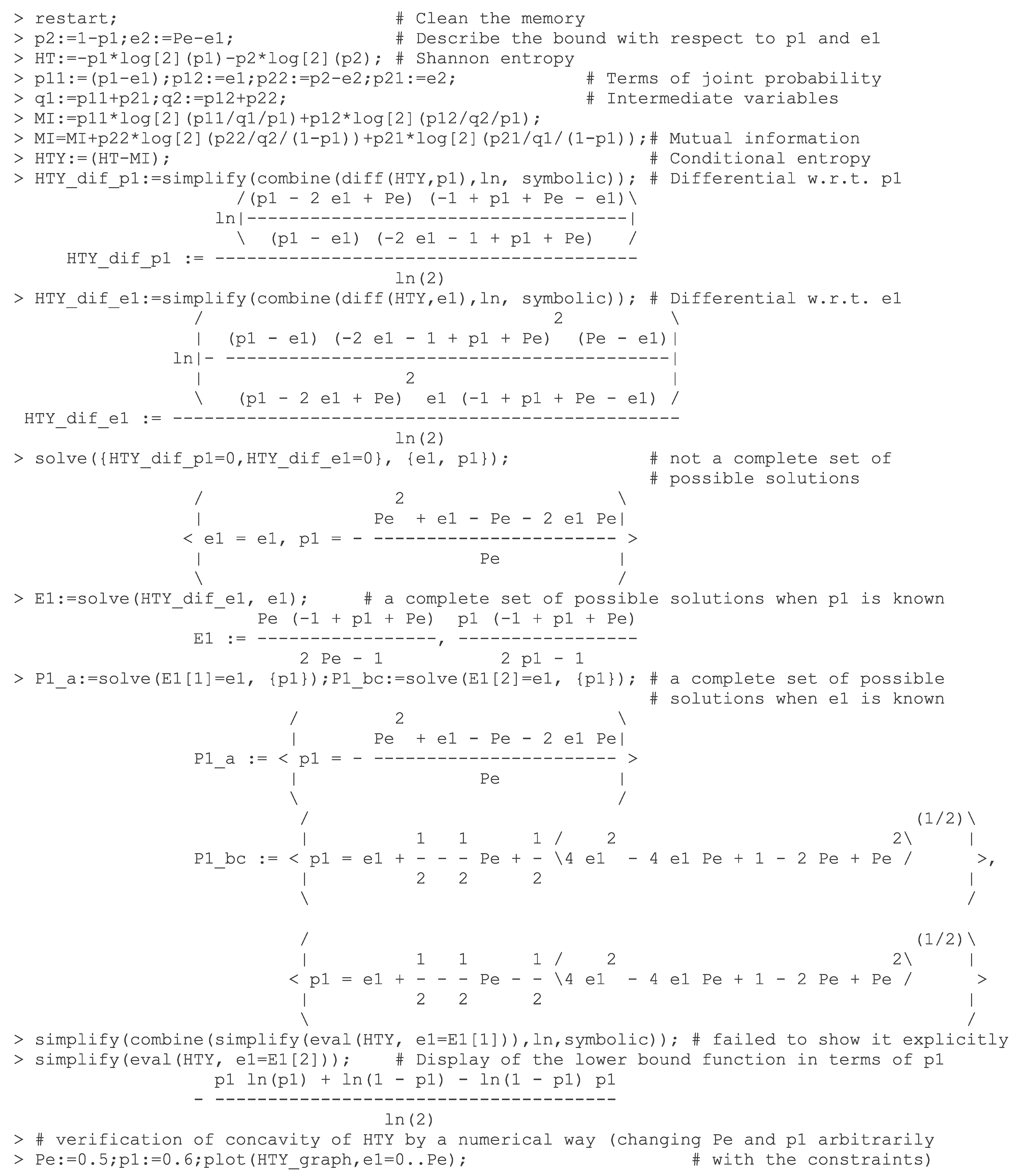
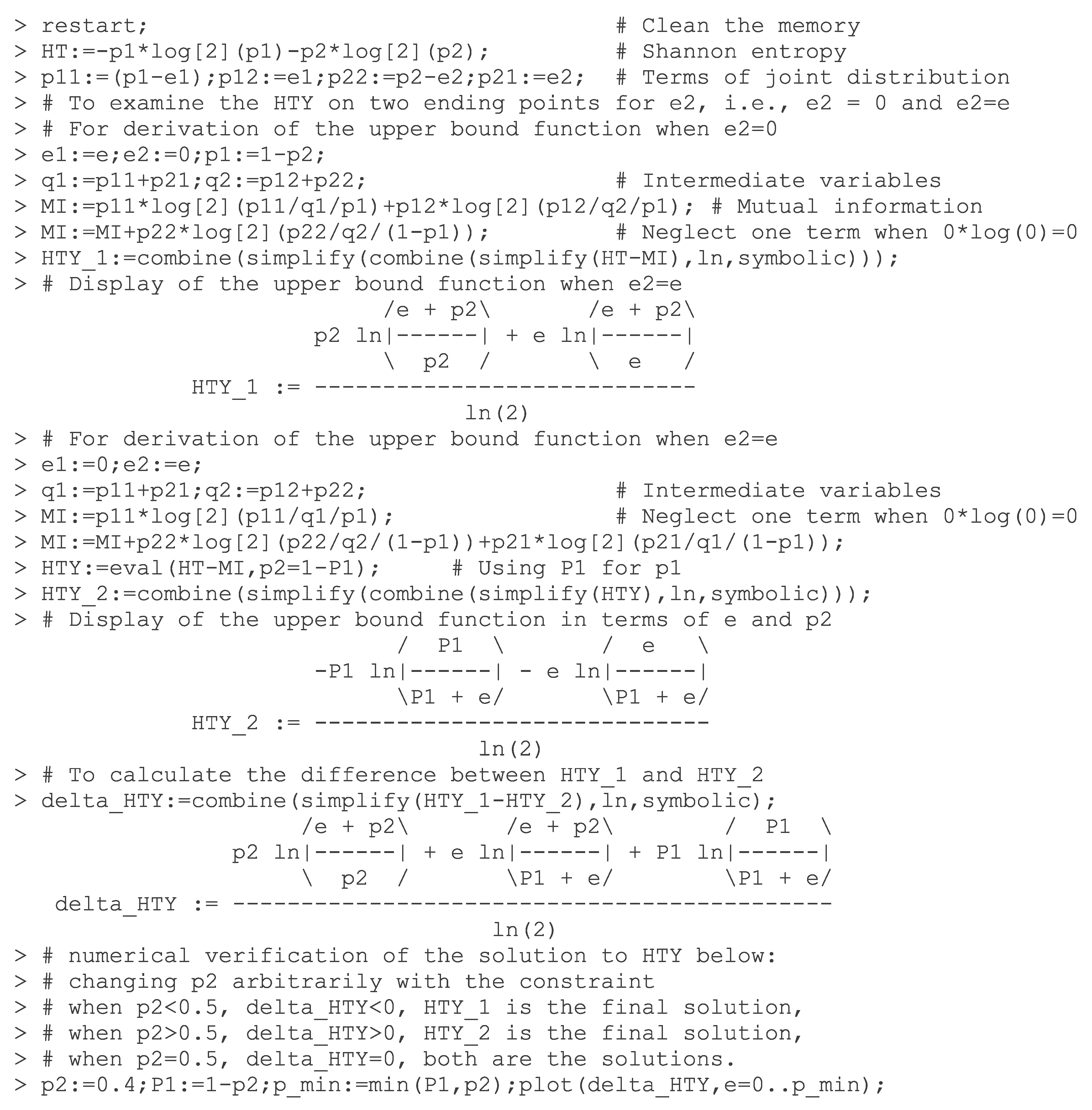
Section 8. The source code from using symbolic software for the derivation is included in
Figure A1 and
Figure A2.
2. Related Works
Two important bounds are introduced first, which form the baselines for the comparisons with the new bounds. They were both derived from inequality conditions [
1,
8]. Suppose the random variables
X and
Y representing input and output messages (out of
m possible messages), and the conditional entropy
representing the average amount of information lost on
X when given
Y [
22]. Fano’s lower bound for the error probability [
1,
22] is given in a form of:
where
is the
error probability (sometimes, also called
error rate or
error for short), and
is the binary entropy function defined by [
23]:
The base of the logarithm is two so that the units are
bits.
The upper bound for the error probability is given by Kovalevskij [
8] in a piecewise linear form [
10]:
where
k is a positive integer number, but defined to be smaller than
m. For a binary classification (
), Fano–Kovalevskij bounds become:
where
denotes an inverse function of
and has no closed-form expression. Hence, we set it as a function form,
, in terms of the variable
. Feder and Merhav [
24] depicted bounds of Equation (4) and presented interpretations on the two specific points from the background of data compression problems.
Studies from the different perspectives have been reported on the bounds between error probability and entropy. The initial difference is made from the entropy definitions, such as Shannon entropy in [
12,
14,
25,
26], and Rényi entropy in [
6,
7,
15]. The second difference is the selection of bound relations, such as “
vs.
” in [
12,
24], “
vs.
” in [
6,
7,
14,
15,
20], “
vs.
” in [
27,
28], and “
vs.
A” in [
25], where
A is the accuracy rate,
and
are the mutual information and normalized mutual information between variables
X and
Y, respectively. Another important study is made on the tightness of bounds. Several investigations [
17,
19,
20,
29] have been reported on the improvement of bound tightness. Recently, a study in [
26] suggested that an upper bound from the Bayesian errors should be added, which is generally neglected in the bound analysis.
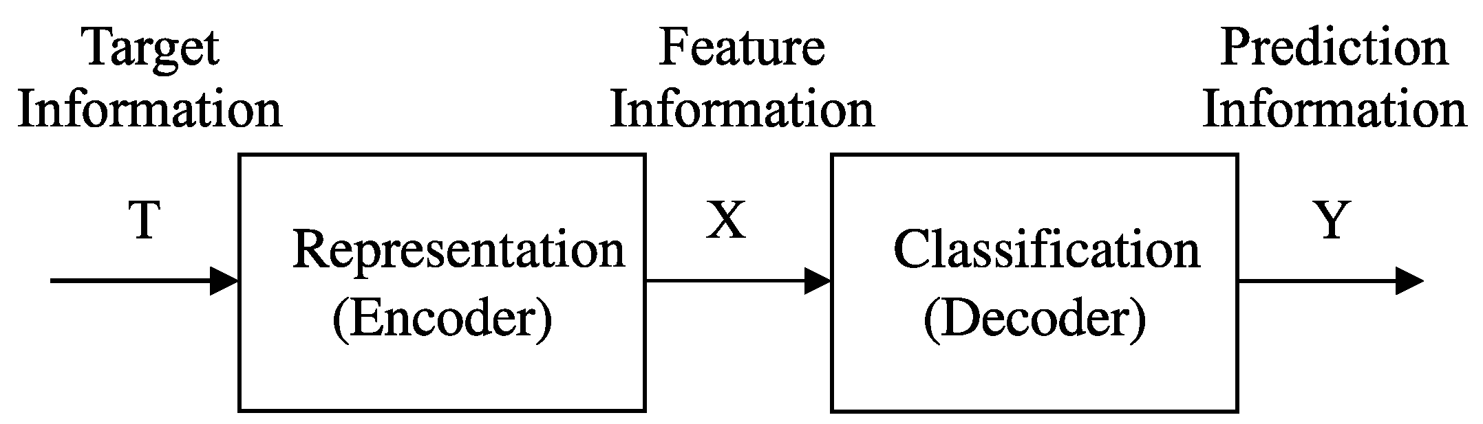
3. Binary Classifications and Related Definitions
Classifications can be viewed as one component in pattern recognition systems [
30].
Figure 1 shows a schematic diagram of the pattern recognition systems. The first unit in the systems is termed
representation in the present problem background but called
encoder in communication background. This unit processes the tasks of
feature selection, or
feature extraction. The second unit is called
classification or
classifier in applications. Three sets of variables are involved in the systems, namely,
target variable T,
feature variables X, and
prediction variable Y. While
T and
Y are univariate discrete random variables for representing labels of the samples,
X can be high-dimensional random variables either in forms of discrete, continuous, or their combinations.
In this work, binary classifications are considered as a case study because they are more fundamental in applications. Sometimes, multi-class classifications are processed by binary classifiers [
31]. In this section, we will present several necessary definitions for the present case study. Let
be a random sample satisfying
, which is in a
d-dimensional feature space and will be classified. The true (or target) state
t of
is within the finite set of two classes,
, and the prediction (or output) state
is within the two classes,
, where
f is a function for classifications. Let
be the
prior probability of class
and
be the
conditional probability density function (or
conditional probability) of
given that it belongs to class
.
Definition 1. (Bayesian error in binary classification) In a binary classification, the
Bayesian error, denoted by
, is defined by [
30]:
where
is the
decision region for class
. The two regions are determined by the Bayesian rule:
In statistical classifications, the Bayesian error is the
theoretically lowest probability of error [
30].
Definition 2. (Non-Bayesian error) The
non-Bayesian error, denoted by
, is defined to be any error which is larger than the Bayesian error, that is:
for the given information of
and
.
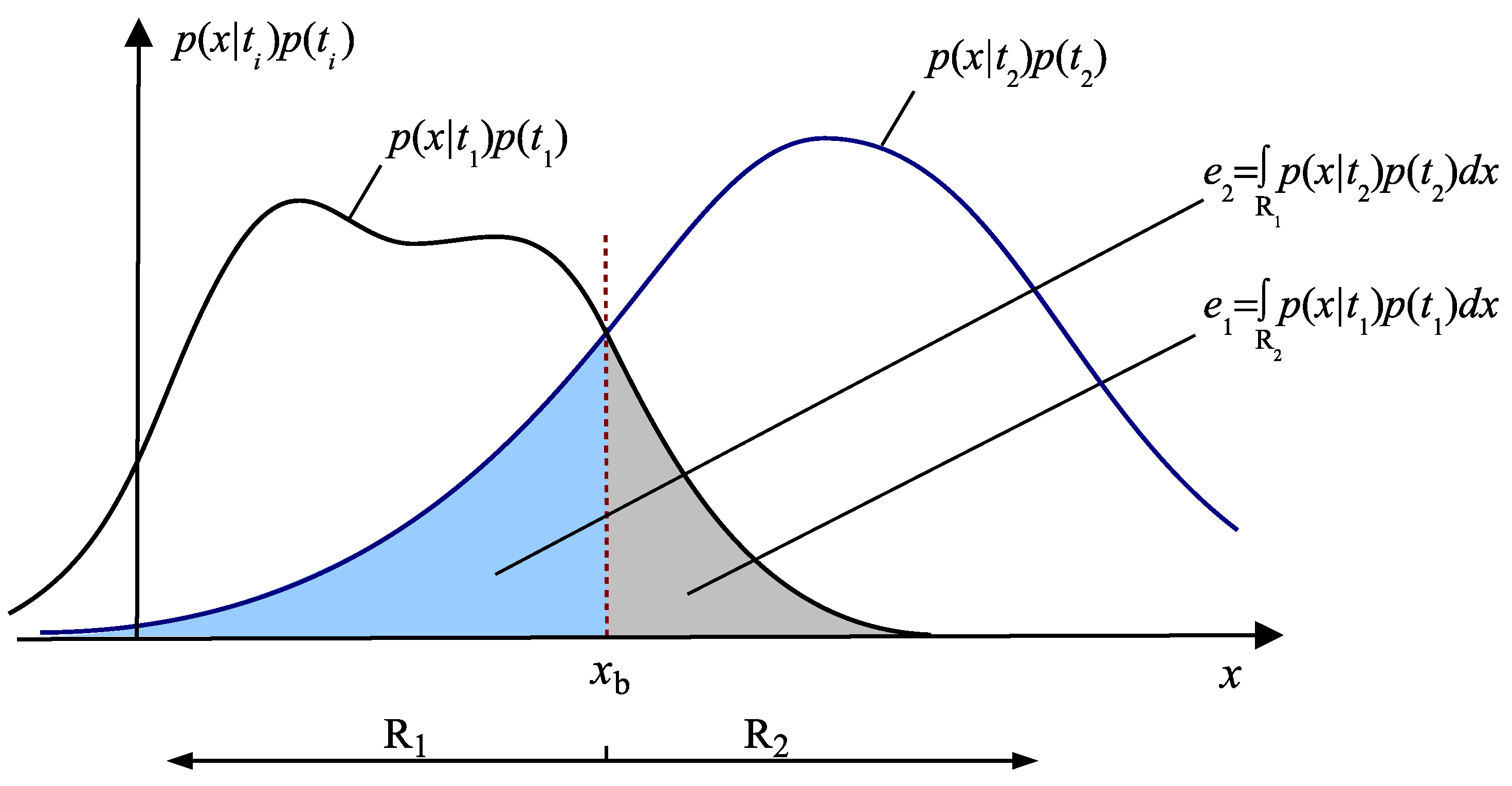
Remark 1. Based on the definitions above, for the given joint distribution, the Bayesian error is unique, but the non-Bayesian errors are multiple.
Figure 2 shows the Bayesian
decision boundary,
, on a univariate feature variable
x for equal priors. The Bayesian error is
. Any other decision boundary different from
will generate the non-Bayesian error for
.
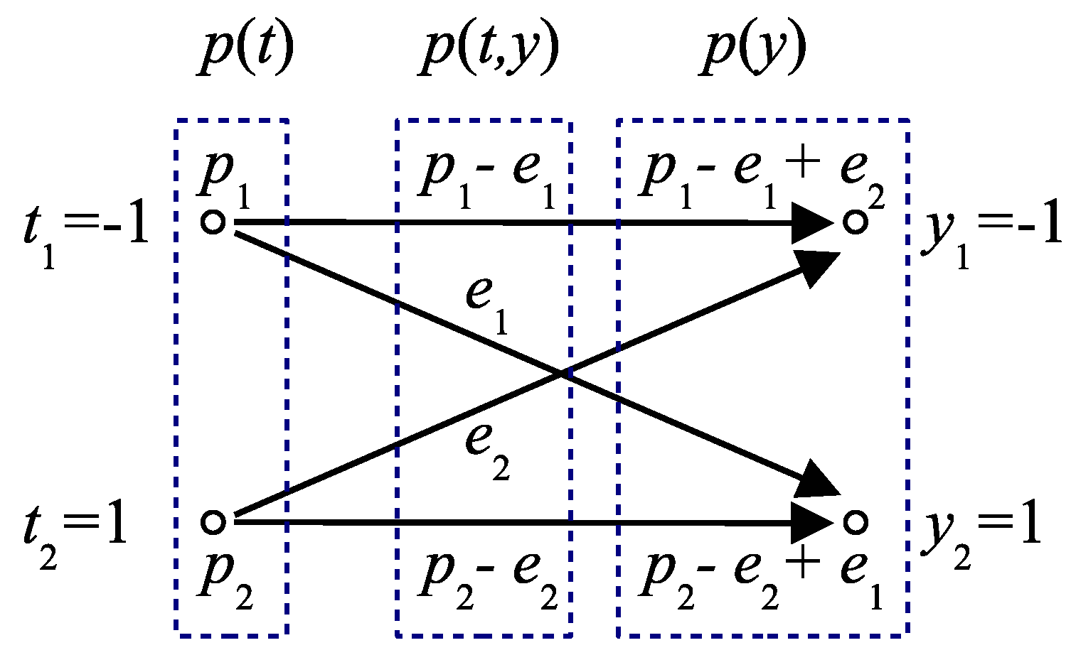
In a binary classification, the
joint distribution,
, is given in a general form of:
where
and
are the prior probabilities of Class 1 and Class 2, respectively; their associated errors (also called
error components) are denoted by
and
.
Figure 3 shows a graphic diagram of the probability transformation between target variable
T and prediction variable
Y via their joint distribution
in a binary classification. The constraints in Equation (8) are given by [
30]:
In this work, we use
e to denote error probability, or error variable, for representing either the Bayesian error or non-Bayesian error. They are calculated from the same formula:
Definition 3. (Minimum and maximum error bounds in binary classifications) Classifications suggest the minimum error bound as:
where the subscript
min denotes the minimum value. The maximum error bound for the Bayesian error in binary classifications is [
26]:
where the symbol
min denotes a
minimum operation. For the non-Bayesian error, its maximum error bound becomes
The Equations from Equations (11) to (13) describe the initial ranges of Bayesian and non-Bayesian errors respectively. When they share the same minimum, their maximums are always different.
Remark 2. For a given set of joint distributions in the bound studies, one may fail to tell if it is the solution from using the Bayesian rule or not. Only when , we can say the set is corresponding to the non-Bayesian solution.
In a binary classification, the
conditional entropy,
, is calculated from the joint distribution in Equation (8):
where
is a
binary entropy of the random variable
T, and
is
mutual information between variables
T and
Y.
Remark 3. When a joint distribution is given, its associated conditional entropy is uniquely determined. However, for the given , it is generally unable to reach a unique solution to but receives multiple solutions shown later in this work.
Definition 4. (Admissible point, admissible set, and their properties in diagram of entropy and error probability) In a given diagram of entropy and error probability, if a point in the diagram is possibly to be realized from a non-empty set of joint distributions for the given classification information, it is defined to be an admissible point. Otherwise, it is a non-admissible point. All admissible points will form an admissible set (or admissible region(s)), which is enclosed by the bounds (also called boundary). If every point located on the boundary is admissible (or non-admissible), we call this admissible set closed (or open). If only a partial portion of boundary points is admissible, the set is said to be partially closed. For an admissible point with the given conditions, if it is realized only by a unique joint distribution, it is called a one-to-one mapping point. If more than one joint distribution is associated to the same admissible point, it is called a one-to-many mapping point.
We consider that classifications present an exemplary justification of raising the first issue in
Section 1 about the bound studies. The main reason behind the issue is that a single index of error probability may not be sufficient for dealing with classification problems. For example, when processing class-imbalance problems [
32,
33], we need to distinguish
error types. In other words, for the same error probability
e (or even the same admissible point), we are required to know the error components of
and
as well. Suppose one encounters a medical diagnosis problem, where
(say,
) generally represents the
majority class for
healthy persons (labeled with
negative or −1 in
Figure 3), and
(
) the
minority class for
abnormal persons (labeled with
positive or 1). A class-imbalance problem is then formed. While
(also called
type I error ) is tolerable (say,
),
(or
type II error) seems intolerable (say,
) because abnormal persons are considered to be “
healthy”. In class-imbalance problems, the performance measure from error probability may become useless. For example, a classification having
does not support a high, yet reasonable, performance. Hence, from either theoretical or application viewpoint, it is necessary for establishing relations between bounds and joint distributions, which can provide error type information within error probability for better interpretations to the bounds.
4. Lower and Upper Bounds for Bayesian Errors
In this work, we select the bound relations between entropy and error probability. Furthermore, the bounds and their associated error components are also given by the following two theorems in a context of binary classifications.
Theorem 1. (Lower bound and associated error components) The lower bound in a diagram of “ vs.
” and the associated error components with constraints Equations (9) and (12) are given by:where is the conditional entropy of T when given Y, and is called the lower bound function (or lower bound). However, one can only achieve the closed-form solution on its inverse function, , not on itself. Proof. Based on Equation (
14), the lower bound function is derived from the following definition:
where we take
e for the input variable in the derivations Equation (16) describes the function of the maximum
with respect to
e, and the function needs to satisfy the general constraints of joint distributions in Equation (9).
seems to be governed by the four variables from
and
in Equation (
14). However, only two independent parameter variables determine the solutions of Equations (14) and (16). The variable reduction from four to two is due to the two specific constrains imposed between parameters, that is,
and
. When we set
and
as two independent variables, (16) is then equivalent to solving the following problem:
is a continuous and differentiable function with respect to the two variables. A differential approach is applied analytically for searching the
critical points of the optimizations in Equation (17). We achieve the two differential equations below and set them to be zeros:
By solving them simultaneously, we obtain the three pairs of the critical points through analytical derivations:
The highest order of each variable, and , in Equation (18) is four. However, we can see the quadratic component within the first function in Equation (18), , will degenerate the total solution order from four to three. Therefore, the three pairs of critical points exhibit a complete set of possible solutions to the problem in Equation (17). The final solution should be the pair(s) that satisfies both the maximum with respect to for the given and the Equations constraints (9) and (12). Due to high complexity of the nonlinearity of the second-order partial differential equations on , it seems intractable to examine the three pairs analytically for the final solution.
To overcome the difficulty above, we apply a symbolic software tool, Maple™9.5 (a registered trademark of Waterloo Maple, Inc.), for a
semi-analytical solution to the problem (see Maple code in
Figure A1). For simplicity and without loss of generality in classifications, we consider
and
are known constants in the function. The concavity property of
with respect to
in the ranges defined in Equation (19a) is confirmed numerically by varying data on
and
. Hence, a maximum solution on
is always received from the possible solutions of the critical points. Among them, only Equation (19a) satisfies the constraints to be the final solution. When
is set, the expression of
is known as shown in Equation (15c). The singular case is given specifically and the solution of
is obtained when
is used in the error expressions. ☐
Remark 4. Theorem 1 achieves the same lower bound found by Fano [
1] (
Figure 4), which is general for finite alphabets (or multiclass classifications). One specific relation to Fano’s bound is given by the
marginal probability (see (2-144) in [
2]):
which is termed
sharp for attaining equality in Equation (1) [
2]. We call Fano’s bound an
exact lower bound because every point on it is sharp. The sharp conditions in terms of error components in Equation (15c) are a special case of the study in [
20], and can be derived directly from their Theorem 1.
Theorem 2. (Upper bound and associated error components) The upper bound and the associated error components with constraints Equations (9) and (12) are given by:where is called the upper bound function (or upper bound). The closed-form solution can be achieved only on its inverse function, . Proof. The upper bound function is obtained from solving the following equation:
Because the concavity property holds for
with respect to
as discussed in the proof of Theorem 1, the possible solutions of
should be located at the two ending points, that is, either at
or at
. We can take the point which produces the smaller
and satisfies the constraints as the final solution. The solution from Maple code in
Figure A2 confirms the closed-form expressions in (21). ☐
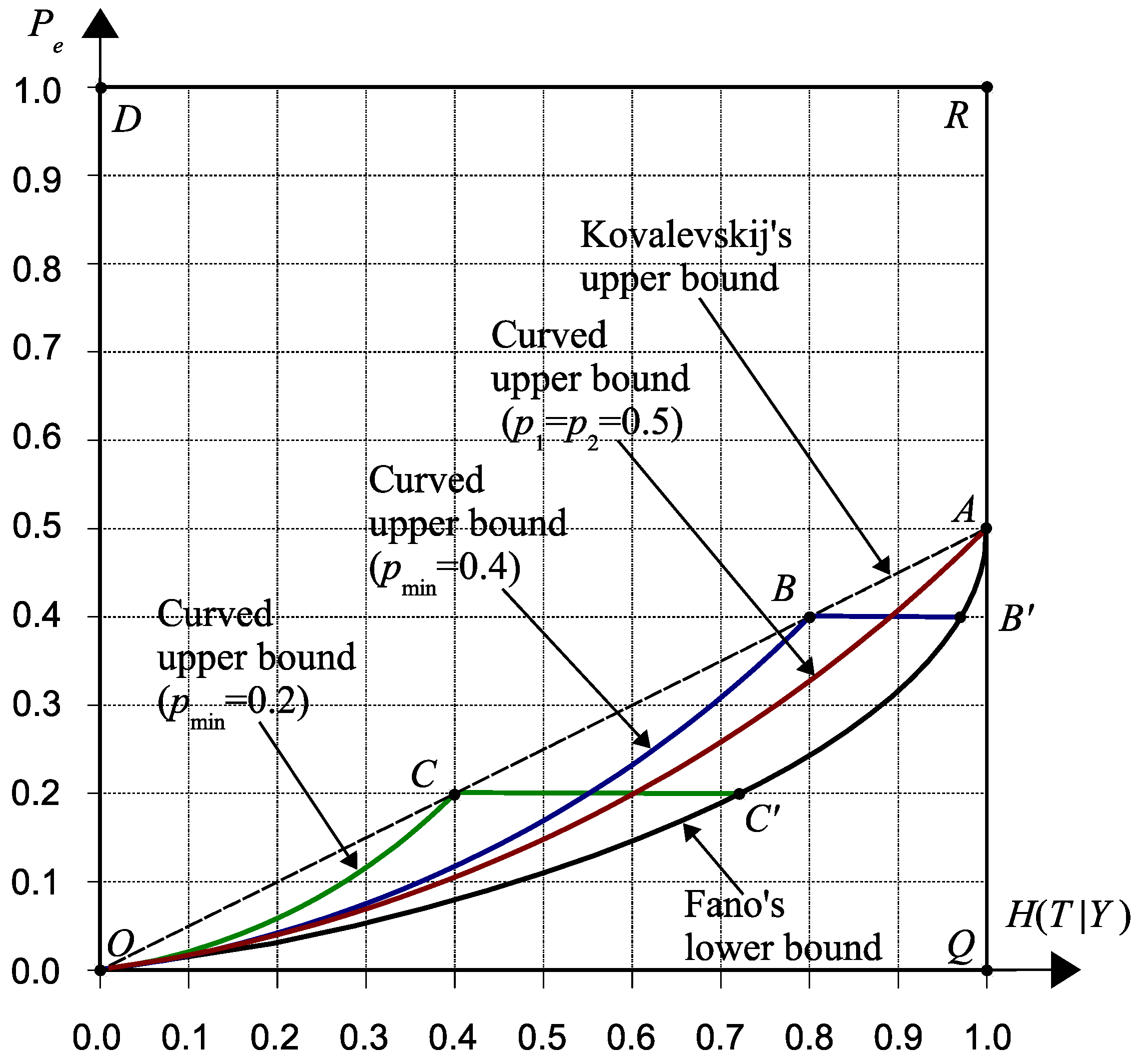
Remark 5. Theorem 2 describes a novel set of upper bounds which is in general
tighter than Kovalevskij’s bound [
8] for binary classifications (
Figure 4). For example, when
is given, the upper bounds defined in Equation (21) shows a curve “
” plus a line “
”. Kovalevskij’s upper bound, given by a line “
”, is sharp only at Point
O and Point
C. The solution in Equation (21c) confirms an advantage of using the proposed optimization approach in derivations so that a closed-form expression of the exact bound is possibly achieved.
In comparison, Kovalevskij’s upper bound described in Equation (3) is general for multiclass classifications. This bound misses a general relation to error components like Equation (21c), although the relation is restricted to a binary state. For distinguishing from the Kovalevskij’s upper bound, we also call
a
curved upper bound. The new
linear upper bound,
, shows the maximum error for the Bayesian decisions in binary classifications [
26], which is also equivalent to the solution of a blind guess when using the maximum-likelihood decision [
30]. If
, the upper bound becomes a single curved one.
Remark 6. The lower and upper bounds defined by Equations (15) and (21) form a closed admissible region in the diagram of “ vs. ”. The shape of the admissible region changes depending on a single parameter of .
5. Lower and Upper Bounds for Non-Bayesian Errors
In classification problems, the Bayesian errors can be realized only if one has the exact information about all probability distributions of classes. The assumption above is generally impossible in real applications. In addition, various classifiers are designed by employing the non-Bayesian rules or resulted in non-Bayesian errors, from the conventional decision trees, artificial neural networks, and supporting vector machines [
30], to the emerging deep learning [
34]. Therefore, the analysis of the non-Bayesian errors presents significant interests in classification studies, although the conventional information theory does not distinguish the error types.
Definition 5. (Label-switching in binary classifications) In binary classifications, a label-switching operation is an exchange between two labels. Suppose the original joint distribution is denoted by:
A label-switching operation will change the prediction labels in
Figure 3 to be
and
, and generate the following joint distribution:
Proposition 1. (Invariant property from label-switching) The related entropy measures, including , , , and , will be invariant to labels, or unchanged from a label-switching operation in binary classifications. However, the error e will be changed to be .
Proof. Substituting the two sets of joint distributions in Equation (23) into each entropy measure formula respectively, one can obtain the same results. The error change is obvious. ☐
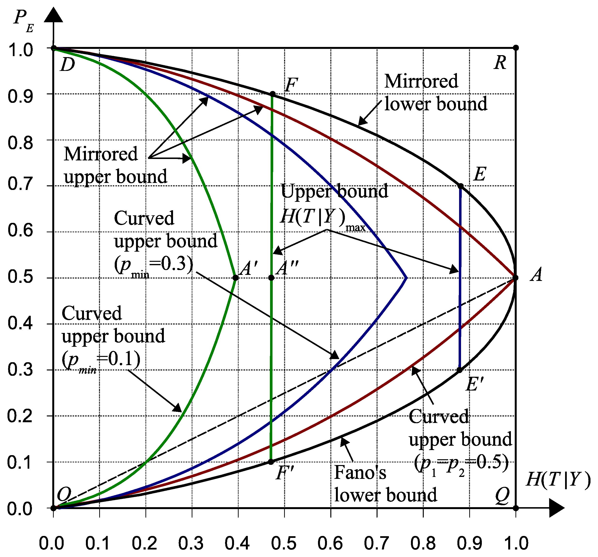
Theorem 3. (Lower bound and upper bound for non-Bayesian error without information of and ) In a context of binary classifications, when information about and is unknown (say, before classifications), the lower bound and upper bound for the non-Bayesian error with constraints Equations (9) and (13) are given by:where we call the upper bound in Equation (24a), , the general upper bound (or mirrored lower bound), which is a mirror of Fano’s lower bound with the mirror axis along . Both bounds share the same expression for calculating the associated error components in Equation (24c). When , their components, and , correspond to the lower bound, otherwise, to the upper bound. Proof. When the error probability is relaxed by Equation (13), all possible solutions in Equation (19) are applicable but within the special ranges respectively. Suppose an admissible point is located at the lower bound which shows . By a label-switching operation, one can obtain the mirrored admissible point at , which is located at the mirrored lower bound. Proposition 1 suggests both points share the same value of . Because is the smallest one for the given conditional entropy , its mirrored point is the biggest one for creating the general upper bound. ☐
Remark 7. Han and Verdù [
16] achieved Fano’s bound from the joint distributions by including the independent condition
[
2]. The condition will only lead to the last set of error equations in Equation (24c), not to the complete sets. In addition, the set is only applicable to the non-Bayesian errors, not to the Bayesian ones except for a special case in Equation (20). Equation (24c) confirms again the advantage of using the optimization in derivations which achieves the complete sets of solutions to describe Fano’s bound for non-Bayesian errors.
Remark 8. The bounds from Equation (24) are derived only when
and
are given. They exist even one does not have such information. In this situation, Fano’s lower bound, its mirror bound, and the axis of
form an admissible region, denoted by a boundary “
” in
Figure 5. The axis of
encloses the region, but only Points O and D are admissible. Hence, the admissible region is partially closed.
Theorem 4. (Admissible region(s) for non-Bayesian error with known information of and ) In binary classifications, when information about and is known, a closed admissible region for the non-Bayesian error with constraints Equations (9) and (13) is generally formed (Figure 5) by Fano’s lower bound, the general upper bound, the curved upper bound , the mirrored upper bound of , and the upper bound . For the bound, its associated error components are given by: Proof. Following the proof in Theorem 3, one can get the mirrored upper bound of
. The upper bound
is calculated from the condition of
[
2]. For the given
and
,
is a constant. Because
also implies a minimization of
in Equation (
14), its associated error components can be obtained from the following equivalent relation (see (11) in [
35]):
☐
Remark 9. Equations (25) and (26) equivalently represent a zero value for the mutual information, which suggests
no correlation [
30] or
statistically independent [
2] between two variables
T and
Y.
Remark 10. When information of
and
is known, the admissible region(s) is much compact than that when without such information. The shape of the admissible region(s) is fully dependent on a single parameter
. For example, if
, the area is enclosed by the four-curve-one-line boundary “
” in
Figure 5. However, if
, two admissible areas are formed. They are “
” and “
”, respectively.
6. Classification Interpretations to Some Key Points
For a better understanding of the theoretical insights between the bounds and errors, some key points shown in
Figure 4 and
Figure 5 are discussed. Those key points may hold special features in classifications. Novel interpretations are expected from the following discussions.
Point O: This point represents a zero value of
. It also suggests an
exact classification without any error (
) by a specific setting of the joint distribution:
This point is always admissible and independent of error types.
Point A: This point shows the maximum ranges of
for
class-balanced classifications (
). Three specific classification settings can be obtained for representing this point. The two settings from Equation (24c) are actually
no classification:
They also indicate
zero information [
36] from the classification decisions. The other setting is a
random guessing from Equation (25):
For the Bayesian errors, this point is always included by both Fano’s bound and Kovalevskij’s bound. However, according to the upper bounds defined in Equation (21a), this point is non-admissible whenever the relation holds. For the non-Bayesian errors, the point is either admissible or non-admissible depending on the given information about and . This example suggests that the admissible property of a point should generally rely on the given information in classifications.
Point D: This point occurs for the non-Bayesian classifications in a form of:
In this case, one can exchange the labels for a perfect classification.
Point B: This point is located at the corner formed by the curved and linear upper bounds, with
and
. In apart from Point
O, this is another point obtained from Equation (21) that locates at Kovalevskij’s upper bound. The point can be realized from either Bayesian or non-Bayesian classifications. Suppose
for the Bayesian classifications. One will achieve Point
B by Equation (21):
for a one-to-one mapping. In other words, this point is uniquely determined by Equation (31) and only corresponding to
within the Bayesian classifications. If non-Bayesian classifications are considered, this point becomes a one-to-many mapping and shows
. For example, one can get another setting of joint distribution from solving
for
first. Then, by substituting the relations of
and
into Equation (25), one can get the error components, that is,
and
, for the new setting of joint distribution on Point
B.
Point
B becomes non-admissible when
(
Figure 4), which means no joint distribution exists to satisfy Equation (9). In this situation, we can understand why the new upper bound is generally tighter than Kovalevskij’s upper bound.
Point : The point is with
and
in the diagram (
Figure 4). It is exactly located at the lower bound and is able to produce a one-to-many mapping for either the Bayesian errors or non-Bayesian errors. One specific setting in terms of the Bayesian errors is:
which suggests zero information from classifications. More settings can be obtained from Equation (15). For example, if given
,
and
, one can have:
Another setting is for the balanced error components:
The non-Bayesian errors will enlarge the set of one-to-many mapping for an admissible point due to the relaxed condition of Equation (13). Equation (24c) will be applicable for deriving a specific setting when
and
e are given. For example, two settings can be obtained:
for representing the same Point
.
Remark 11. One can observe that Equations (35) and (36) will lead to a zero mutual information, but Equations (33) and (34) are not. The observations reveal new interpretations about Fano’s bound in association with two situations in the independent properties of the variables, which have not been reported before.
Points E and : All points located at the general upper bound, like Point
E, will correspond to the settings from the non-Bayesian errors. If a point located at the lower bound, say
, it can represent settings from either the Bayesian or non-Bayesian errors depending on the given information in classifications. Points
E and
form the mirrored points. Their settings can be connected by a relation in Equation (23) but are not necessary. For example, one specific setting for Point
with
and
is:
the other for Point
E with
and
is:
They are mirrored to each other but have no label-switching relation.
Points and : When
and
, Points
and
form a pair as the ending points for the given conditions. Supposing
and
, one can get the specific setting for Point
from Equation (21c):
and one for Point
from Equation (25):
Points Q and R: The two points are specific due to their positions in the diagrams. For either type of errors, both points are non-admissible in the diagrams, because no joint distribution exists in binary classifications which can represent the points.
8. Discussions
To emphasize the importance of the study, we present discussions below from the perspective of machine learning in the context of big-data classifications. We consider that binary classifications will be one of key techniques to implement a
divide-and-conquer strategy [
39] for efficiently processing large quantities of data. Class-imbalance problems with extremely-skewed ratios are mostly formed from a
one-against-other division scheme [
31] in binary classifications. Researchers and users, of course, concern error components in types for performance evaluations [
32]. The knowledge of bounds in relation to error components is desirable for theoretical and application purposes.
From a viewpoint of machine learning, the bounds derived in this work provide a basic solution to link learning targets between error and entropy in the related studies.
Error-based learning is more conventional because of its compatibility with our intuitions in daily life, such as “
trial and error”. Significant studies have been reported under this category. In comparison,
information-based learning [
40] is relatively new and uncommon in some applications, such as classifications. Entropy is not a well-accepted concept related to our intuition in decision making. This is one of the reasons why the learning target is chosen mainly based on error, rather than on entropy. However, error is an empirical concept, whereas entropy is theoretical and general [
41]. In [
35], we demonstrated that entropy can deal with both notions of
error and
reject in abstaining classifications. Information-based learning [
40] presents a promising and wider perspective for exploring and interpreting learning mechanisms.
When considering all sides of the issues stemming from machine learning studies, we believe that “what to learn” is a primary problem. However, it seems that more investigations focused on the issue of “how to learn”, which should be put as the second-level problem. Moreover, in comparison with the long-standing yet hot theme of feature selection, little study has been done from the perspective of learning target selection. We propose that this theme should be emphasized in the study of machine learning. Hence, the relations studied in this work are fundamental and crucial to the extent that researchers, using either error-based or entropy-based approaches, are able to reach a better understanding about its counterpart.

