Bounding Extremal Degrees of Edge-Independent Random Graphs Using Relative Entropy

Abstract

Edge-independent random graphs are a model of random graphs in which each potential edge appears independently with an individual probability. Based on the relative entropy method, we determine the upper and lower bounds for the extremal vertex degrees using the edge probability matrix and its largest eigenvalue. Moreover, an application to random graphs with given expected degree sequences is presented.

1. Introduction

Edge-independent random graphs are random graph models with independent but (possibly) heterogeneous edge probabilities, generalizing the model with constant edge probability introduced by Erdős and Rényi [1,2]. Given a real symmetric matrix $A=\left(p_{ij}\right)\in {\mathbb{R}}^{n\times n}$ with $p_{ij}\in [0,1]$, the edge-independent random graph model $G_n\left(p_{ij}\right)$ [3] is defined as a random graph on the vertex set $\left[n\right]=\{1,2,\cdots ,n\}$, which includes each edge $(i,j)$ with probability $p_{ij}$ independently. Clearly, the classical Erdős-Rényi random graphs and the Chung–Lu models [4] with given expected degrees are two special examples of $G_n\left(p_{ij}\right)$.

Edge-independent random graphs are applicable in a range of areas such as modeling of social networks, and detection of community structures [5,6], etc. The number of interacting nodes is typically large in practical applications, and it is appropriate to investigate the statistical properties of parameters of interest. The Estrada index and the normalized Laplacian Estrada index of $G_n\left(p_{ij}\right)$ for large n are examined in [7]. The problem of bounding the difference between eigenvalues of A and those of the adjacency matrix of $G_n\left(p_{ij}\right)$, together with its Laplacian spectra version, has been studied intensively recently; see, e.g., [3,8,9]. It is revealed in [9] that large deviation from the expected spectrum is caused by vertices with extremal degrees, where abnormally high-degree and low-degree vertices are obstructions to concentration of the adjacency and the Laplacian matrices, respectively. A regularization technique is employed to address this issue.

Relative entropy [10] is a key notion in quantum information theory, ergodic theory, and statistical mechanics. It measures the difference between two probability distributions; see e.g., [11,12,13,14,15,16,17] for various applications of relative entropy on physical, chemical and engineering sciences.

Inspired by the above consideration, we in this paper study the extremal degrees of the edge-independent random graph $G_n\left(p_{ij}\right)$ in the thermodynamic limit, namely, as n tends to infinity. Our approach is based on concentration inequalities, where the notation of relative entropy plays a critical role. We first build the theory for maximum and minimum degrees for $G_n\left(p_{ij}\right)$ in Section 2, and then present an application for the random graph model $G\left(w\right)$ with given expected degree sequence w and a discussion regarding possible future direction in Section 3. Various combinatorial and geometric properties of $G\left(w\right)$ including the hyperbolicity and warmth have been reported; see, e.g., [18,19,20].

2. Bounds for Maximum and Minimum Degrees

Recall that $A=\left(p_{ij}\right)\in {\mathbb{R}}^{n\times n}$ is a real symmetric matrix. Its eigenvalues can be ordered as ${\lambda }_1\left(A\right)\ge {\lambda }_2\left(A\right)\ge \cdots \ge {\lambda }_n\left(A\right)$. Given a graph $G\in G_n\left(p_{ij}\right)$, let $\Delta \left(G\right)$ and $\delta \left(G\right)$ be its maximum and minimum degrees, respectively. The maximum expected degree of G is denoted by $\Delta \left(A\right)$, which is equivalent to the maximum row sum of A. Let $\overline{p}=max\left\{p_{ij}\right\}$ and $\underline{p}=min\left\{p_{ij}\right\}$ represent the maximum and minimum elements, respectively, in A. We say that a graph property $\mathcal{P}$ holds in $G_n\left(p_{ij}\right)$ asymptotically almost surely (a.a.s.) if the probability that a random graph $G\in G_n\left(p_{ij}\right)$ has $\mathcal{P}$ converges to 1 as n goes to infinity.

Theorem 1. 

For an edge-independent random graph G, suppose that $\Delta \left(A\right)\gg {ln}^{4}n$. Then

$${\lambda }_1\left(A\right)-(2+o\left(1\right))\sqrt{\Delta \left(A\right)}\le \Delta \left(G\right)\le (1+o\left(1\right))n\overline{p},a.a.s.$$

(1)

Proof. 

The lower bound is straightforward since

$$\Delta \left(G\right)\ge {\lambda }_1\left(G\right)\ge {\lambda }_1\left(A\right)-(2+o\left(1\right))\sqrt{\Delta \left(A\right)}a.a.s.$$

(2)

by employing Theorem 1 in [3].

For the upper bound, we set $d_i=d_i\left(G\right)$ as the degree of vertex i in G. By construction, $d_i\sim {\sum }_{j=1}^{n}Ber\left(p_{ij}\right)$ follows the sum of n independent Bernoulli distributions. If $\overline{p}=1$, the upper bound in Equation (1) holds true trivially. Therefore, we assume $\overline{p}<1$ in the sequel.

For any non-decreasing function $f\left(x\right)$ on the interval $[0,n]$, the Markov inequality [2] implies that for $\overline{p}<a<1$,

$$\mathbb{P}(d_i\ge an)=\mathbb{P}(f\left(d_i\right)\ge f\left(an\right))\le \frac{\mathbb{E}\left(f\left(d_i\right)\right)}{f\left(an\right)}=\frac{{\sum }_{k=0}^{n}f\left(k\right){\overline{p}}^k{(1-\overline{p})}^{n-k}}{f\left(an\right)}.$$

(3)

By choosing $f\left(x\right)={\left(a/\overline{p}\right)}^x{\left((1-a)/(1-\overline{p})\right)}^{n-x}$, we obtain from (3) that

$$\mathbb{P}(\Delta \left(G\right)\ge an)\le \sum _{i=1}^n\mathbb{P}(d_i\ge an)\le n{e}^{-nEnt(a,\overline{p})},$$

(4)

where $Ent(a,\overline{p})=aln(a/\overline{p})+(1-a)ln\left((1-a)/(1-\overline{p})\right)$ is the so-called relative entropy [10].

Recall the Taylor expansion of $ln(1+x)=x-x^2/2+x^3/3-x^4/4+\cdots$. For any $\epsilon >0$, we have $ln((1-\overline{p})/(1-(1+\epsilon )\overline{p}))\le (1-\overline{p})/(1-(1+\epsilon )\overline{p})-1$ and

$$\begin{array}{c}\hfill (1+\epsilon )ln(1+\epsilon )-\epsilon \ge (1+\epsilon )\left(\epsilon -\frac{{\epsilon }^2}{2}\right)-\epsilon =\frac{1}{2}{\epsilon }^2(1-\epsilon ).\end{array}$$

(5)

Now, we choose $\epsilon >0$ satisfying $a=(1+\epsilon )\overline{p}<1$. Therefore, if $\epsilon =o\left(1\right)$ as $n\to \infty$, the above comments and the inequality (4) yield

$$\mathbb{P}(\Delta \left(G\right)\ge (1+\epsilon )n\overline{p})\le n{e}^{-\frac{1}{2}n\overline{p}{\epsilon }^2(1+o\left(1\right))}.$$

(6)

By assumption, we have $n\overline{p}\gg {ln}^{4}n$. We choose $\epsilon =\left({ln}^{2}n\right)/\sqrt{n\overline{p}}=o\left(1\right)$. Hence, the estimate (6) implies that $\Delta \left(G\right)\le (1+o\left(1\right))n\overline{p}$ asymptotically almost surely, which concludes the proof of the upper bound.  ☐

Remark 1. 

The lower bound in (1) is best possible according to [3]. The upper bound in (1) is also essentially best possible. Indeed, suppose that there exists $0<q<\overline{p}$ satisfying $\Delta \left(G\right)\le (1+o(1\left)\right)nq$ a.a.s.. Given an $i_0\in \left[n\right]$, we define $p_{i_{0}j}=\overline{p}$ for all j. Hence, $\mathbb{E}\left(d_{i_0}\right)>qn$. Using the Chernoff bound, we deduce that $\mathbb{P}(d_{i_0}>(1+o\left(1\right))nq)=1-o\left(1\right)$, which contradicts the assumption.

Remark 2. 

The use of Markov’s inequality in (3) is of course reminiscent of the Chernoff bound, which is a common tool in bounding tail probabilities [2]. However, we mention that the relative entropy $Ent(a,\overline{p})$ here plays an essential role that cannot be simply replaced by the Chernoff-type bounds. The Chernoff’s inequality (see, e.g., Lem. 1 in [4]) gives

$$\mathbb{P}\left(d_i\ge (1+\epsilon )\sum _{j=1}^n{p}_{ij}\right)\le e^{-\left({\sum }_{j=1}^n{p}_{ij}\right){\epsilon }^2/3}\le e^{-n\underline{p}{\epsilon }^2/3},$$

(7)

which may produce a fit upper bound only if $\underline{p}=\overline{p}$. The similar comments can be applied to Theorem 2 below for the minimum degree of $G_n\left(p_{ij}\right)$.

Remark 3. 

Notice that $\Delta \left(A\right)\le n\overline{p}$. It is easy to see that the upper bound $\Delta \left(G\right)\le (1+o\left(1\right))n\overline{p}$ holds a.a.s. provided $\overline{p}\gg (lnn)/n$. In fact, it suffices to take $\epsilon =2\sqrt{(lnn)/n\overline{p}}$ in the above proof.

Remark 4. 

If $p_{ij}=p$ for all i and j, the edge-independent model $G_n\left(p_{ij}\right)$ reduces to the Erdős-Rényi random graph $G_n\left(p\right)$ (with possible self-loops; however, this is not essential throughout this paper). Since $\Delta \left(A\right)={\lambda }_1\left(A\right)=np$, Theorem 1 implies that for $G\in G_n\left(p\right)$, if $np\gg {ln}^{4}n$, we have $\Delta \left(G\right)=(1+o(1\left)\right)np$ a.a.s.. However, this result is already known to be true under an even weaker condition, namely, $np\gg lnn$ (see, e.g., p.72, Cor. 3.14 in [1], [21]). It is viable to expect that our Theorem 1 holds as long as $\Delta \left(A\right)\gg lnn$. Unfortunately, we do not have a proof presently.

This also lends support to the conjecture made in [3] that Theorem 1 therein (regarding the behavior of adjacency eigenvalues of edge-independent random graphs) holds when $\Delta \left(A\right)\gg lnn$. A partial solution in this direction can be found in [8].

Theorem 2. 

Let G be an edge-independent random graph.

(A) 

If $\underline{p}\gg (lnn)/n$, then $(1+o\left(1\right))n\underline{p}\le \delta \left(G\right)\le (1+o\left(1\right))n\overline{p}a.a.s.;$

(B) 

If $\Delta \left(A\right)\gg {ln}^{4}n$, then $\delta \left(G\right)\le n-{\lambda }_1\left(A\right)+(2+o\left(1\right))\sqrt{\Delta \left(A\right)}a.a.s..$

Proof. 

The statement (B) holds directly from Theorem 1 by noting that $\delta \left(G\right)=n-\Delta \left(G^c\right)$, where $G^c$ is the complement of G. Since $\overline{p}\ge \underline{p}\gg (lnn)/n$ and $\delta \left(G\right)\le \Delta \left(G\right)$, the upper bound in the statement (A) follows immediately from Remark 3. It remains to prove the lower bound of the statement (A).

To show the lower bound, we address three cases separately.

Case 1. $\underline{p}=1$. It it clear that $\delta \left(G\right)\ge (1+o\left(1\right))n\underline{p}$ a.a.s. in this case.

Case 2. $1-\underline{p}=O\left({(lnn)}^{1/3}/n^{1/3}\right)$.

For any non-decreasing function $g\left(x\right)$ on the interval $[0,n]$, the Markov inequality indicates that for $0<a<\underline{p}<1$,

$$\begin{array}{ccc}\hfill \mathbb{P}(d_i\le an)& =& \mathbb{P}(g(n-d_i)\ge g(n-an))\le \frac{\mathbb{E}\left(g(n-d_i)\right)}{g(n-an)}\hfill \\ & =& \frac{{\sum }_{k=0}^{n}g(n-k){\underline{p}}^k{(1-\underline{p})}^{n-k}}{g(n-an)}.\hfill \end{array}$$

(8)

By choosing $g\left(x\right)={\left(a/\underline{p}\right)}^{n-x}{\left((1-a)/(1-\underline{p})\right)}^x$, we obtain from (8) that

$$\mathbb{P}(d_i\le an)\le e^{-nEnt(a,\underline{p})},$$

(9)

where $Ent(a,\underline{p})$ is the relative entropy defined in the proof of Theorem 1.

In the following, we choose $a\to 1$ and $1-\underline{p}\ll 1-a$ as $n\to \infty$. Hence, from (9) we obtain

$$\begin{array}{ccc}\hfill \mathbb{P}\left(\delta \right(G)\le an)& \le & nexp\left(-n\left(aln(a/\underline{p})+(1-a)ln((1-a)/(1-\underline{p}))\right)\right)\hfill \\ & \le & nexp\left(-n\left((1-a)ln((1-a)/(1-\underline{p}))-2(1-a)\right)+lnn\right),\hfill \end{array}$$

(10)

where in the second inequality we have used the following estimation

$$\begin{array}{cc}\hfill e^{-\frac{2(1-a)}{a}}& \le 1-\frac{2(1-a)}{a}+\frac{2{(1-a)}^2}{a^2}=\frac{1/(1-a)-3}{1/(1-a)-1}+\Theta \left({(1-a)}^2\right)\hfill \\ & \le \frac{1/(1-a)-1}{1/(1-a)-(1-\underline{p})/(1-a)}=\frac{a}{\underline{p}}.\hfill \end{array}$$

(11)

By assumption we set $1-\underline{p}\le c{(lnn)}^{1/3}/n^{1/3}$ for some $c>0$. By choosing $1-a={(lnn)}^{2/3}/n^{1/3}$, we obtain

$$(1-a)\left(ln\left(\frac{1-a}{1-\underline{p}}\right)-2\right)\ge (1-a)\left(ln\left(\frac{(1-a)}{c}{\left(\frac{n}{lnn}\right)}^{\frac{1}{3}}\right)-2\right)\ge \frac{2lnn}{n}.$$

(12)

Combining (10) and (12) we arrive at $\mathbb{P}(\delta \left(G\right)\le an)\le e^{-lnn}\to 0$ as $n\to \infty$.

Finally, by our choice of parameters, $a/\underline{p}=(1/(1-a)-1)/(1/(1-a)-(1-\underline{p})/(1-a))\to 1$ as $n\to \infty$. Hence, $an=(1+o\left(1\right))n\underline{p}$, which completes the proof in this case.

Case 3. $1-\underline{p}\gg {(lnn)}^{1/3}/n^{1/3}$.

Notice that $G^c$ can be viewed as a random graph in $G_n(1-p_{ij})$. Hence, the same arguments towards (4) imply that

$$\mathbb{P}(\Delta \left(G^c\right)\ge (1+\epsilon )(1-\underline{p})n)\le n{e}^{-nEnt\left((1+\epsilon )(1-\underline{p}),1-\underline{p}\right)}$$

(13)

for any $\epsilon >0$ satisfying $(1+\epsilon )(1-\underline{p})<1$.

In the following, we take $o\left(1\right)=\epsilon \ll \underline{p}$. Thus, the relative entropy in (13) can be bounded below as

$$\begin{array}{cc}\hfill Ent\left((1+\epsilon )(1-\underline{p}),1-\underline{p}\right)=& (1+\epsilon )(1-\underline{p})ln(1+\epsilon )+(\underline{p}-\epsilon +\underline{p}\epsilon )ln\left(1-\frac{\epsilon (1-\underline{p})}{\underline{p}}\right)\hfill \\ \hfill \ge & (1+\epsilon )(1-\underline{p})\left(\epsilon -\frac{{\epsilon }^2}{2}\right)\hfill \\ & +(\underline{p}-\epsilon +\underline{p}\epsilon )\left(-\frac{\epsilon (1-\underline{p})}{\underline{p}}-\frac{{\epsilon }^2{(1-\underline{p})}^2}{2{\underline{p}}^2}-\frac{{\epsilon }^3{(1-\underline{p})}^3}{{\underline{p}}^3}\right)\hfill \\ \hfill =& \frac{{\epsilon }^2}{2\underline{p}}\left((1-\underline{p})-c_1\left(\epsilon +\frac{\epsilon }{\underline{p}}\right)+O\left(\underline{p}{\epsilon }^2\right)\right),\hfill \end{array}$$

(14)

where $c_1>0$ is a constant. Combining (13) and (14) we obtain

$$\begin{array}{cc}\hfill \mathbb{P}(\Delta \left(G^c\right)\ge (1+\epsilon )(1-\underline{p})n)\le & exp\left(-\frac{n{\epsilon }^2}{2\underline{p}}\left((1-\underline{p})-c_1\left(\epsilon +\frac{\epsilon }{\underline{p}}\right)+O\left(\underline{p}{\epsilon }^2\right)\right)+lnn\right)\hfill \\ \hfill \le & exp\left(-\frac{c_{2}n{\epsilon }^2}{2\underline{p}}(1-\underline{p})+lnn\right),\hfill \end{array}$$

(15)

where $c_2>0$ is a constant. Here, in the second inequality of (15), we have employed the assumptions $1-\underline{p}\gg {(lnn)}^{1/3}/n^{1/3}$ and $\underline{p}\gg (lnn)/n$.

Take $\epsilon =\sqrt{3\underline{p}(lnn)/\left(c_2(1-\underline{p})n\right)}$ in the inequality (15). It is direct to check that $\epsilon \to 0$ and $\epsilon /\underline{p}\to 0$ as $n\to \infty$ under our assumptions. Hence, we have $\mathbb{P}(\Delta \left(G^c\right)\ge (1+\epsilon )(1-\underline{p})n)=o\left(1\right)$, and

$$\delta \left(G\right)=n-\Delta \left(G^c\right)\ge n-(1+\epsilon )(1-\underline{p})n=(1+o\left(1\right))n\underline{p}a.a.s..$$

(16)

The last equality holds since $o\left(1\right)=\epsilon \ll \underline{p}$. The proof is then complete.  ☐

Remark 5. 

Similarly as in Remark 1, the upper and lower bounds of Theorem 2 are essentially best possible.

Remark 6. 

When $p_{ij}=p$ for all i and j, Theorem 2 reduces to the fact for Erdős-Rényi model that $\delta \left(G\right)=(1+o(1\left)\right)np$ a.a.s. provided $p\gg (lnn)/n$. This result is already known (see, e.g., p.152 in [2]) and is proved by a more sophisticated method called Stein’s method. A more or less similar approach appears in [21].

3. An Application to Random Graphs with Given Expected Degrees

The random graph model $G\left(w\right)$ with given expected degree sequence $w=(w_1,w_2,\cdots ,w_n)$ is defined by including each edge between vertex i and j independently with probability $p_{ij}=w_i{w}_j/Vol\left(G\right)$, where the volume $Vol\left(G\right)={\sum }_{i=1}^n{w}_i$ [4,18]. By definition we have $\Delta \left(A\right)=w_{max}:={max}_{1\le i\le n}{w}_i$, $\overline{p}=w_{max}^2/Vol\left(G\right)$ and $\underline{p}=w_{min}^2/Vol\left(G\right)$, where $w_{min}:={min}_{1\le i\le n}{w}_i$. Moreover, let the second-order volume and the expected second-order average degree be ${Vol}_2\left(G\right)={\sum }_{i=1}^n{w}_i^2$ and $\tilde{w}={Vol}_2\left(G\right)/Vol\left(G\right)$, respectively.

An application of Theorem 1 to $G\left(w\right)$ yields the following corollary on the maximum degree of $G\left(w\right)$.

Corollary 1. 

For a random graph $G\in G\left(w\right)$, suppose that $w_{max}\gg {ln}^{4}n$. Then

$$\tilde{w}-(2+o\left(1\right))\sqrt{w_{max}}+o\left(1\right)\le \Delta \left(G\right)\le (1+o\left(1\right))\frac{n{w}_{max}^2}{Vol\left(G\right)},a.a.s.$$

(17)

Proof. 

The results follow immediately from Theorem 1 by noting that ${\lambda }_1\left(A\right)\ge \tilde{w}+o\left(1\right)$ (see, e.g., p.163, Lem. 8.7 in [18]).  ☐

Analogously, the following result is for the minimum degree of $G\left(w\right)$.

Corollary 2. 

Let G be a random graph in $G\left(w\right)$.

(A) 

If $w_{min}^2\gg Vol\left(G\right)(lnn)/n$, then

$$(1+o\left(1\right))\frac{n{w}_{min}^2}{Vol\left(G\right)}\le \delta \left(G\right)\le (1+o\left(1\right))\frac{n{w}_{max}^2}{Vol\left(G\right)}a.a.s.;$$

(18)

(B) 

If $w_{max}\gg {ln}^{4}n$, then

$$\delta \left(G\right)\le n-\tilde{w}+(2+o\left(1\right))\sqrt{w_{max}}+o\left(1\right)a.a.s..$$

(19)

To illustrate the availability of the above results, we study two numerical examples.

Example 1. 

Consider the random graph model $G\left(w\right)$ with $w_1=\cdots =w_{n/2}={ln}^{4}n$ and $w_{n/2}=\cdots =w_n={ln}^{5}n$. This model is more or less similar to homogeneous Erdős-Rényi random graphs. It is straightforward to check that all conditions in Corollary 1 and Corollary 2 hold. In Table 1, we compare the theoretical bounds of maximum degrees obtained in Corollary 1 with numerical values using Matlab software. The analogous results for minimum degrees are reported in Table 2. We observe that the simulations are in line with the theory. It turns out that the upper bound for the maximum degree and the lower bound for the minimum degree are more accurate.

Table 1. Maximum degree $\Delta \left(G\right)$ of $G\in G\left(w\right)$ with $w=({ln}^{4}n,\cdots ,{ln}^{4}n,{ln}^{5}n,\cdots ,{ln}^{5}n)$ (with half of the numbers being ${ln}^{4}n$). The theoretical upper and lower bounds are calculated from Corollary 1. Numerical results are based on average over 20 independent runs.

n	Theoretical Lower Bound	$\Delta \left(G\right)$	Theoretical Upper Bound
$9.8\times {10}^5$	$4.683\times {10}^5-(2+o\left(1\right))706.85+o\left(1\right)$	$7.260\times {10}^5$	$(1+o\left(1\right))9.317\times {10}^5$
$9.9\times {10}^5$	$4.701\times {10}^5-(2+o\left(1\right))708.15+o\left(1\right)$	$7.283\times {10}^5$	$(1+o\left(1\right))9.352\times {10}^5$
$10.0\times {10}^5$	$4.718\times {10}^5-(2+o\left(1\right))709.44+o\left(1\right)$	$7.305\times {10}^5$	$(1+o\left(1\right))9.387\times {10}^5$
$10.1\times {10}^5$	$4.735\times {10}^5-(2+o\left(1\right))710.72+o\left(1\right)$	$7.327\times {10}^5$	$(1+o\left(1\right))9.421\times {10}^5$
$10.2\times {10}^5$	$4.752\times {10}^5-(2+o\left(1\right))711.99+o\left(1\right)$	$7.351\times {10}^5$	$(1+o\left(1\right))9.455\times {10}^5$

Table 1. Maximum degree $\Delta \left(G\right)$ of $G\in G\left(w\right)$ with $w=({ln}^{4}n,\cdots ,{ln}^{4}n,{ln}^{5}n,\cdots ,{ln}^{5}n)$ (with half of the numbers being ${ln}^{4}n$). The theoretical upper and lower bounds are calculated from Corollary 1. Numerical results are based on average over 20 independent runs.

n	Theoretical Lower Bound	$\Delta \left(G\right)$	Theoretical Upper Bound
$9.8\times {10}^5$	$4.683\times {10}^5-(2+o\left(1\right))706.85+o\left(1\right)$	$7.260\times {10}^5$	$(1+o\left(1\right))9.317\times {10}^5$
$9.9\times {10}^5$	$4.701\times {10}^5-(2+o\left(1\right))708.15+o\left(1\right)$	$7.283\times {10}^5$	$(1+o\left(1\right))9.352\times {10}^5$
$10.0\times {10}^5$	$4.718\times {10}^5-(2+o\left(1\right))709.44+o\left(1\right)$	$7.305\times {10}^5$	$(1+o\left(1\right))9.387\times {10}^5$
$10.1\times {10}^5$	$4.735\times {10}^5-(2+o\left(1\right))710.72+o\left(1\right)$	$7.327\times {10}^5$	$(1+o\left(1\right))9.421\times {10}^5$
$10.2\times {10}^5$	$4.752\times {10}^5-(2+o\left(1\right))711.99+o\left(1\right)$	$7.351\times {10}^5$	$(1+o\left(1\right))9.455\times {10}^5$

Table 2. Minimum degree $\delta \left(G\right)$ of $G\in G\left(w\right)$ with $w=({ln}^{4}n,\cdots ,{ln}^{4}n,{ln}^{5}n,\cdots ,{ln}^{5}n)$ (with half of the numbers being ${ln}^{4}n$). The theoretical upper and lower bounds are calculated from Corollary 2. Numerical results are based on average over 20 independent runs.

n	Theoretical Lower Bound	$\delta \left(G\right)$	Theoretical Upper Bound
$9.8\times {10}^5$	$(1+o\left(1\right))4.896\times {10}^3$	$1.826\times {10}^4$	$5.117\times {10}^5+(2+o\left(1\right))706.85+o\left(1\right)$
$9.9\times {10}^5$	$(1+o\left(1\right))4.907\times {10}^3$	$1.829\times {10}^4$	$5.200\times {10}^5+(2+o\left(1\right))708.15+o\left(1\right)$
$10.0\times {10}^5$	$(1+o\left(1\right))4.918\times {10}^3$	$1.832\times {10}^4$	$5.282\times {10}^5+(2+o\left(1\right))709.44+o\left(1\right)$
$10.1\times {10}^5$	$(1+o\left(1\right))4.929\times {10}^3$	$1.834\times {10}^4$	$5.365\times {10}^5+(2+o\left(1\right))710.72+o\left(1\right)$
$10.2\times {10}^5$	$(1+o\left(1\right))4.940\times {10}^3$	$1.837\times {10}^4$	$5.448\times {10}^5+(2+o\left(1\right))711.99+o\left(1\right)$

Table 2. Minimum degree $\delta \left(G\right)$ of $G\in G\left(w\right)$ with $w=({ln}^{4}n,\cdots ,{ln}^{4}n,{ln}^{5}n,\cdots ,{ln}^{5}n)$ (with half of the numbers being ${ln}^{4}n$). The theoretical upper and lower bounds are calculated from Corollary 2. Numerical results are based on average over 20 independent runs.

n	Theoretical Lower Bound	$\delta \left(G\right)$	Theoretical Upper Bound
$9.8\times {10}^5$	$(1+o\left(1\right))4.896\times {10}^3$	$1.826\times {10}^4$	$5.117\times {10}^5+(2+o\left(1\right))706.85+o\left(1\right)$
$9.9\times {10}^5$	$(1+o\left(1\right))4.907\times {10}^3$	$1.829\times {10}^4$	$5.200\times {10}^5+(2+o\left(1\right))708.15+o\left(1\right)$
$10.0\times {10}^5$	$(1+o\left(1\right))4.918\times {10}^3$	$1.832\times {10}^4$	$5.282\times {10}^5+(2+o\left(1\right))709.44+o\left(1\right)$
$10.1\times {10}^5$	$(1+o\left(1\right))4.929\times {10}^3$	$1.834\times {10}^4$	$5.365\times {10}^5+(2+o\left(1\right))710.72+o\left(1\right)$
$10.2\times {10}^5$	$(1+o\left(1\right))4.940\times {10}^3$	$1.837\times {10}^4$	$5.448\times {10}^5+(2+o\left(1\right))711.99+o\left(1\right)$

Example 2. 

Power-law graphs, which are prevalent in real-life networks, can also be constructed based on the Chung–Lu model $G\left(w\right)$ [18]. Given a scaling exponent β, an average degree $d:=Vol\left(G\right)/n$, and $w_{max}$, a power-law random graph $G\left(w\right)$ is defined by taking $w_i=c{i}^{-1/(\beta -1)}$ for $i_0\le i<i_0+n$, where

$$c=\frac{\beta -2}{\beta -1}d{n}^{\frac{1}{\beta -1}}\mathrm{and}{i}_0=n{\left(\frac{d(\beta -2)}{w_{max}(\beta -1)}\right)}^{\beta -1}.$$

(20)

We choose $\beta =2.5$, $w_{max}=\sqrt{n}$, and $d={(lnn)}^2$. It is direct to check that the conditions in Corollary 1 and Corollary 2 hold.

In Figure 1 we show the maximum and minimum degrees as well as the theoretical bounds for $G\left(w\right)$ with different number of vertices. Note that the upper bound in (19) is worse than that in (18) for this example. We thus invoke the same upper bounds for both $\Delta \left(G\right)$ and $\delta \left(G\right)$ in Figure 1.

Figure 1. Extremal degree versus the number of vertices n. The theoretical upper and lower bounds are from (17) and (18). Each data point is obtained by means of a mixed ensemble averaging of 30 independent runs of 10 graphs yielding a statistically ample sampling.

Figure 1. Extremal degree versus the number of vertices n. The theoretical upper and lower bounds are from (17) and (18). Each data point is obtained by means of a mixed ensemble averaging of 30 independent runs of 10 graphs yielding a statistically ample sampling.

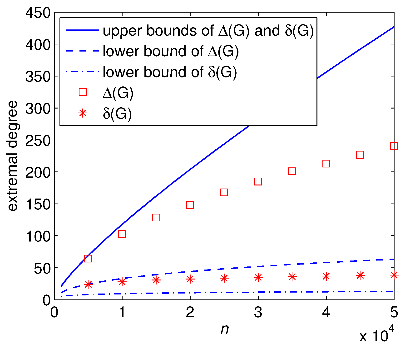
We observe interestingly, as in Example 1, that the upper bound for the maximum degree and the lower bound for the minimum degree seem to be more accurate. As is known that large deviation phenomena are normally associated with a global hard constraint which fights against a local soft constraint. We contend that the deviations from the expected degree sequence are due here to a fight of the constrained degree sequence with the imposed edge-independency.

Figure 2. A depiction of the small-world graph $S(n,p,C_{2k})$ with $n=16$, $p=0$, and $k=3$.

Figure 2. A depiction of the small-world graph $S(n,p,C_{2k})$ with $n=16$, $p=0$, and $k=3$.

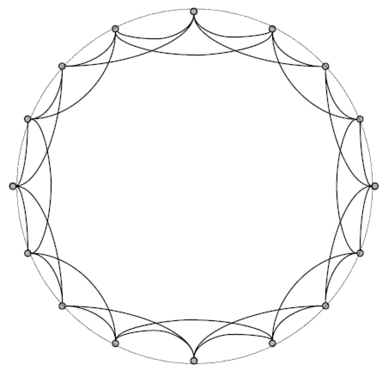
As a follow up work, inspired by the above examples, it would be of interest to identify all the graphs that are close to the theoretical upper or lower bounds. As an illustrating example, we consider the small-world graph $G=S(n,p,C_{2k})$ ($k\ge 1$) studied in [22,23], which can be viewed as the join of a random graph $G_n\left(p\right)$ and a ring on n vertices, each of which has edges to precisely k subsequent and k previous neighbors (see, e.g., Figure 2). In the special case of $p\equiv 0$, G becomes a regular graph, and we know that ${\lambda }_1\left(A\right)=\Delta \left(G\right)=2k$, where A is the adjacency matrix of G. If $k\gg {ln}^{4}n$ holds, it follows from Theorem 1 that

$$2k-(2+o\left(1\right))\sqrt{2k}\le 2k\le (1+o\left(1\right))n,a.a.s.$$

(21)

Clearly, the upper bound is close if k is large, while the lower bound tends to be more accurate if k is small. In general, when $p\gg ({ln}^{4}n/)n$ holds, for any $k\ge 1$ it follows from Theorem 1 that

$${\lambda }_1\left(A\right)-(2+o\left(1\right))\sqrt{2k+(n-2k-1)p}\le \Delta \left(G\right)\le (1+o\left(1\right))n,a.a.s.$$

(22)

Note that the second largest eigenvalue of the adjacency matrix of $S(n,0,C_{2k})$, which is a circulant matrix, is

$${\lambda }_2\left(A\left(S(n,0,C_{2k})\right)\right)=\frac{sin\left(\pi \right(2k+1)/n)}{sin(\pi /n)}-1=(2+o\left(1\right))k,$$

(23)

as $n\to \infty$. Utilizing the edge version of Cauchy’s interlacing theorem, (22) and (23), we derive the following estimation

$$(2+o\left(1\right))\left(k-\sqrt{2k+(n-2k-1)p}\right)\le \Delta \left(G\right)\le (1+o\left(1\right))n,a.a.s.$$

(24)

The gap between upper and lower bounds can be quite close provided k attains it maximum, namely, $\lfloor (n-1)/2\rfloor$.

References

- Bollobás, B. Random Graphs, 2nd ed.; Cambridge University Press: Cambridge, UK, 2001. [Google Scholar]
- Janson, S.; Łuczak, T.; Ruciński, A. Random Graphs; Wiley: New York, NY, USA, 2000. [Google Scholar]
- Lu, L.; Peng, X. Spectra of edge-independent random graphs. Electron. J. Comb. 2013; arXiv:1204.6207. [Google Scholar]
- Chung, F.; Lu, L. Connected components in random graphs with given expected degree sequences. Ann. Comb. 2002, 6, 125–145. [Google Scholar] [CrossRef]
- Abbe, E.; Sandon, C. Community detection in the general stochastic block model: Fundamental limits and efficient algorithms for recovery. In Proceedings of 56th Annual IEEE Symposium on Foundations of Computer Science, Berkely, CA, USA, 18–20 October 2015.
- Chin, P.; Rao, A.; Vu, V. Stochastic block model and community detection in the sparse graphs: A spectral algorithm with optimal rate of recovery. In Proceedings of JMLR Workshop and Conference, Paris, France, 2–6 July 2015.
- Shang, Y. Estrada and L-Estrada indices of edge-independent random graphs. Symmetry 2015, 7, 1455–1462. [Google Scholar] [CrossRef]
- Lei, J.; Rinaldo, A. Consistency of spectral clustering in stochastic block models. Ann. Stat. 2015, 43, 215–237. [Google Scholar] [CrossRef]
- Le, C.M.; Vershynin, R. Concentration and regularization of random graphs. 2015; arXiv:1506.00669. [Google Scholar]
- Cover, T.M.; Thomas, J.A. Elements of Information Theory; Wiley-Interscience: New York, NY, USA, 1991. [Google Scholar]
- Vedral, V. The role of relative entropy in quantum information theory. Rev. Mod. Phys. 2002, 74. [Google Scholar] [CrossRef]
- Blanco, D.D.; Casini, H.; Hung, L.-Y.; Myers, R.C. Relative entropy and holography. J. High Energy Phys. 2013, 2013. [Google Scholar] [CrossRef]
- Lin, S.; Gao, S.; He, Z.; Deng, Y. A pilot directional protection for HVDC Transmission line based on relative entropy of wavelet energy. Entropy 2015, 17, 5257–5273. [Google Scholar] [CrossRef]
- Gaveau, B.; Granger, L.; Moreau, M.; Schulman, L.S. Relative entropy, interation energy and the nature of dissipation. Entropy 2014, 16, 3173–3206. [Google Scholar] [CrossRef]
- Prehl, J.; Boldt, F.; Essex, C.; Hoffmann, K.H. Time evolution of relative entropies for anomalous diffusion. Entropy 2013, 15, 2989–3006. [Google Scholar] [CrossRef]
- Lods, B.; Pistone, G. Information geometry formalism for the spatially homogeneous Boltzmann equation. Entropy 2015, 17, 4323–4363. [Google Scholar] [CrossRef]
- Mohammad-Djafari, A. Entropy, information theory, information geometry and Bayesian inference in data, signal and image processing and inverse problems. Entropy 2015, 17, 3989–4027. [Google Scholar] [CrossRef]
- Chung, F.; Lu, L. Complex Graphs and Networks; American Mathematical Society: Providence, RI, USA, 2006. [Google Scholar]
- Shang, Y. Non-hyperbolicity of random graphs with given expected degrees. Stoch. Model. 2013, 29, 451–462. [Google Scholar] [CrossRef]
- Shang, Y. A note on the warmth of random graphs with given expected degrees. Int. J. Math. Math. Sci. 2014, 2014, 749856–749860. [Google Scholar] [CrossRef]
- Löwe, M.; Vermet, F. Capacity of an associative memory model on random graph architectures. Bernoulli 2015, 21, 1884–1910. [Google Scholar] [CrossRef]
- Gu, L.; Zhang, X.-D.; Zhou, Q. Consensus and synchronization problems on small-world networks. J. Math. Phys. 2010, 51, 082701. [Google Scholar] [CrossRef]
- Shang, Y. A sharp threshold for rainbow connection in small-world networks. Miskolc Math. Notes 2012, 13, 493–497. [Google Scholar]
© 2016 by the author; licensee MDPI, Basel, Switzerland. This article is an open access article distributed under the terms and conditions of the Creative Commons by Attribution (CC-BY) license (http://creativecommons.org/licenses/by/4.0/).
Share and Cite
MDPI and ACS Style
Shang, Y. Bounding Extremal Degrees of Edge-Independent Random Graphs Using Relative Entropy. Entropy 2016, 18, 53. https://doi.org/10.3390/e18020053
AMA Style
Shang Y. Bounding Extremal Degrees of Edge-Independent Random Graphs Using Relative Entropy. Entropy. 2016; 18(2):53. https://doi.org/10.3390/e18020053
Chicago/Turabian StyleShang, Yilun. 2016. "Bounding Extremal Degrees of Edge-Independent Random Graphs Using Relative Entropy" Entropy 18, no. 2: 53. https://doi.org/10.3390/e18020053
Note that from the first issue of 2016, this journal uses article numbers instead of page numbers. See further details here.