
Sensitivity Analysis of Entropy Generation in Nanofluid Flow inside a Channel by Response Surface Methodology


Abstract
:1. Introduction
2. Problem Statement and Computational Model

- (1)
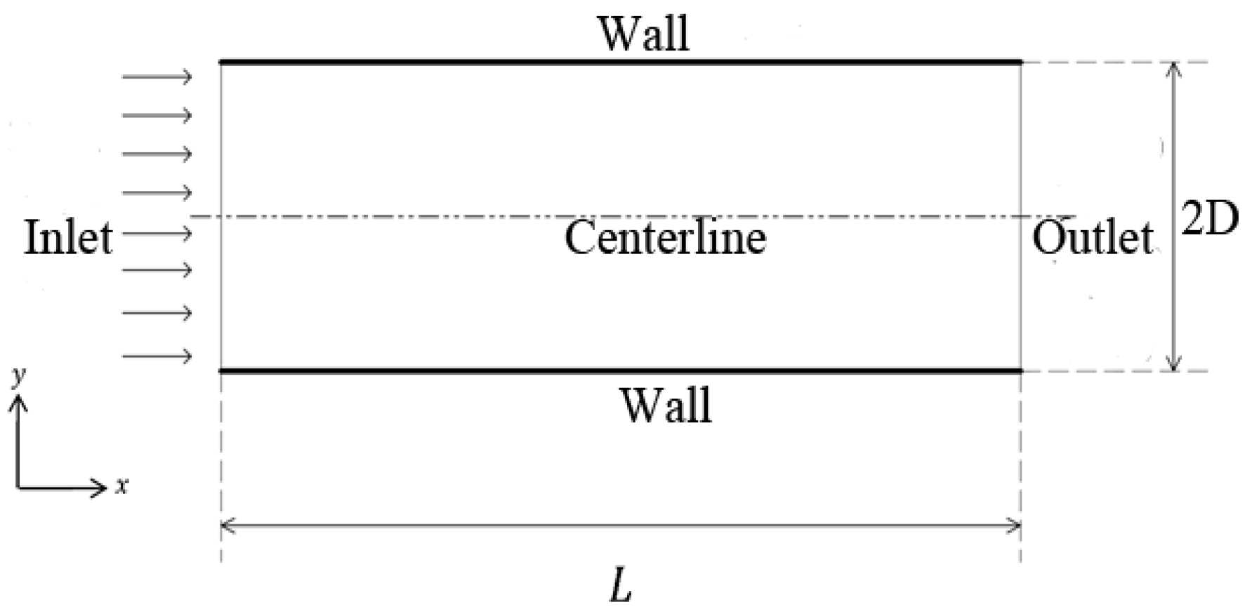
- The flow is considered to be two-dimensional, laminar, steady and incompressible.
- ✓
- This range of Reynolds numbers is significant for designing many devices such as micro devices and compact heat exchangers, which are two important applications of this geometrical (channel).
- ✓
- Higher Reynolds numbers are beyond the limit where two dimensional simulations can be performed [17].
- ✓
- It is safe to drop the viscous dissipation effects in the energy equation at this range of Reynolds number.
- (2)
- Bottom half of the channel is considered in simulation due to the symmetrical shape.
- Conservation of mass equation:
- Energy equation [18]:where Ceff, keff, ρeff and μeff are effective specific heat, conductivity, density and viscosity, respectively.
- The effective density is given by [19]:where ϕ is the solid volume fraction and subscripts f and p indicate fluid and particle, respectively.
- The effective specific heat is measured by using the following equation [20]:
- The effective dynamic viscosity is defined in following form [21]:where N is a non-dimensional function of the nanoparticle diameter, fluid viscosity and solid volume fractions. This function is defined by [21,22]:where δ and VB are the distance between nanoparticles and Brownian velocity of the nanoparticles, respectively. These parameters are defined by [21]:where dp and KB are nanoparticle diameter (= 30 nm) and Boltzmann constant (= 1.38 × 10⁻²³ J·K−1), respectively.
- At the inlet of the channel, a uniform flow is assumed. This boundary is defined by:
- At the channel wall, no slip and constant temperature boundary conditions are imposed. These boundaries are:
- Zero gradient boundary conditions are used at the outlet of the channel [25]. These boundaries are given by:
- Symmetry conditions are assumed at the centerline. These boundaries are given by:


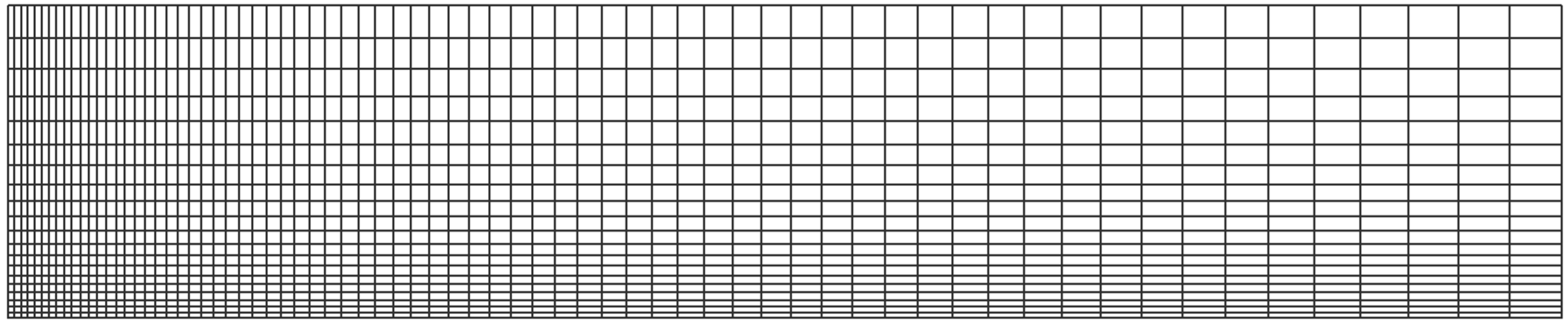
| No. | Grid Size | Nusselt Number | Percentage Difference |
|---|---|---|---|
| 1 | 150 × 20 | 6.057 | 1.6 |
| 2 | 300 × 40 | 6.154 | 1.1 |
| 3 | 600 × 80 | 6.222 | 0.3 |
| 4 | 1200 × 160 | 6.241 | – |

| Parameters Symbol | Level | |||
|---|---|---|---|---|
| −1 | 0 | 1 | ||
| Re | A | 200 | 500 | 800 |
| dp (nm) | B | 30 | 60 | 90 |
| ϕ | C | 0.01 | 0.03 | 0.05 |
| Standard Order | Coded Value | Real Value | Responses | ||||
|---|---|---|---|---|---|---|---|
| A | B | C | Re | dp | ϕ | Nt | |
| 1 | −1 | −1 | −1 | 200 | 30 | 0.01 | 0.014441 |
| 2 | 1 | −1 | −1 | 800 | 30 | 0.01 | 0.043037 |
| 3 | −1 | 1 | −1 | 200 | 90 | 0.01 | 0.013952 |
| 4 | 1 | 1 | −1 | 800 | 90 | 0.01 | 0.031240 |
| 5 | −1 | −1 | 1 | 200 | 30 | 0.05 | 0.015356 |
| 6 | 1 | −1 | 1 | 800 | 30 | 0.05 | 0.059118 |
| 7 | −1 | 1 | 1 | 200 | 90 | 0.05 | 0.014793 |
| 8 | 1 | 1 | 1 | 800 | 90 | 0.05 | 0.038779 |
| 9 | −1 | 0 | 0 | 200 | 60 | 0.03 | 0.014956 |
| 10 | 1 | 0 | 0 | 800 | 60 | 0.03 | 0.041098 |
| 11 | 0 | −1 | 0 | 500 | 30 | 0.03 | 0.037220 |
| 12 | 0 | 1 | 0 | 500 | 90 | 0.03 | 0.027376 |
| 13 | 0 | 0 | −1 | 500 | 60 | 0.01 | 0.026047 |
| 14 | 0 | 0 | 1 | 500 | 60 | 0.05 | 0.033898 |
| 15 | 0 | 0 | 0 | 500 | 60 | 0.03 | 0.031349 |
| 16 | 0 | 0 | 0 | 500 | 60 | 0.03 | 0.031349 |
| 17 | 0 | 0 | 0 | 500 | 60 | 0.03 | 0.031349 |
| 18 | 0 | 0 | 0 | 500 | 60 | 0.03 | 0.031349 |
| 19 | 0 | 0 | 0 | 500 | 60 | 0.03 | 0.031349 |
| 20 | 0 | 0 | 0 | 500 | 60 | 0.03 | 0.031349 |
| Source | DOF | Sum of Squares | Contribution | Adj Mean Squares | F-Value | p-Value | – |
|---|---|---|---|---|---|---|---|
| Model | 9 | 0.002478 | 99.46% | 0.000275 | 203.17 | <0.0001 | Significant |
| Linear | 3 | 0.002249 | 90.26% | 0.000750 | 553.16 | <0.0001 | – |
| A | 1 | 0.001954 | 78.40% | 0.001954 | 1441.41 | <0.0001 | – |
| B | 1 | 0.000185 | 7.43% | 0.000185 | 136.62 | <0.0001 | – |
| C | 1 | 0.000110 | 4.43% | 0.000110 | 81.45 | <0.0001 | – |
| Square | 3 | 0.000039 | 1.58% | 0.000013 | 9.68 | 0.0030 | – |
| AA | 1 | 0.000033 | 1.34% | 0.000023 | 16.72 | 0.0020 | – |
| BB | 1 | 0.000004 | 0.14% | 0.000005 | 3.98 | 0.0074 | – |
| CC | 1 | 0.000002 | 0.09% | 0.000002 | 1.74 | 0.0217 | – |
| Interaction | 3 | 0.000190 | 7.62% | 0.000063 | 46.68 | <0.0001 | – |
| AB | 1 | 0.000121 | 4.85% | 0.000121 | 89.11 | <0.0001 | – |
| AC | 1 | 0.000060 | 2.40% | 0.000060 | 44.09 | <0.0001 | – |
| BC | 1 | 0.000009 | 0.37% | 0.000009 | 6.85 | 0.0026 | – |
| Residual Error | 10 | 0.000014 | 0.54% | 0.000001 | – | – | – |
| Lack-of-Fit | 5 | 0.000014 | 0.54% | 0.000003 | – | – | – |
| Pure Error | 5 | 0.000000 | 0.00% | 0.000000 | – | – | – |
| Total | 19 | 0.002492 | 100% | – | – | – | – |
| Nt | ||
|---|---|---|
| Term | Coefficient | p-Value |
| Constant | 0.03117 | <0.0001 |
| A | 0.01398 | <0.0001 |
| B | −0.00430 | <0.0001 |
| C | 0.00332 | <0.0001 |
| A2 | −0.00287 | 0.0020 |
| B2 | 0.00140 | 0.0740 |
| C2 | −0.00093 | 0.2170 |
| AB | −0.00389 | <0.0001 |
| AC | 0.00273 | <0.0001 |
| BC | −0.00108 | 0.0026 |
| – | R2 = 99.46% | R2-adj = 98.97% |
3. Results and Discussion


| B | C | Sensitivity | ||
|---|---|---|---|---|
| −1 | −1 | 0.0151 | −0.0032 | 0.0044 |
| 0 | 0.0179 | −0.0043 | 0.0044 | |
| 1 | 0.0206 | −0.0054 | 0.0044 | |
| 0 | −1 | 0.0113 | −0.0032 | 0.0033 |
| 0 | 0.0140 | −0.0043 | 0.0033 | |
| 1 | 0.0167 | −0.0054 | 0.0033 | |
| 1 | −1 | 0.0074 | −0.0032 | 0.0022 |
| 0 | 0.0101 | −0.0043 | 0.0022 | |
| 1 | 0.0128 | −0.0054 | 0.0022 | |
4. Conclusions
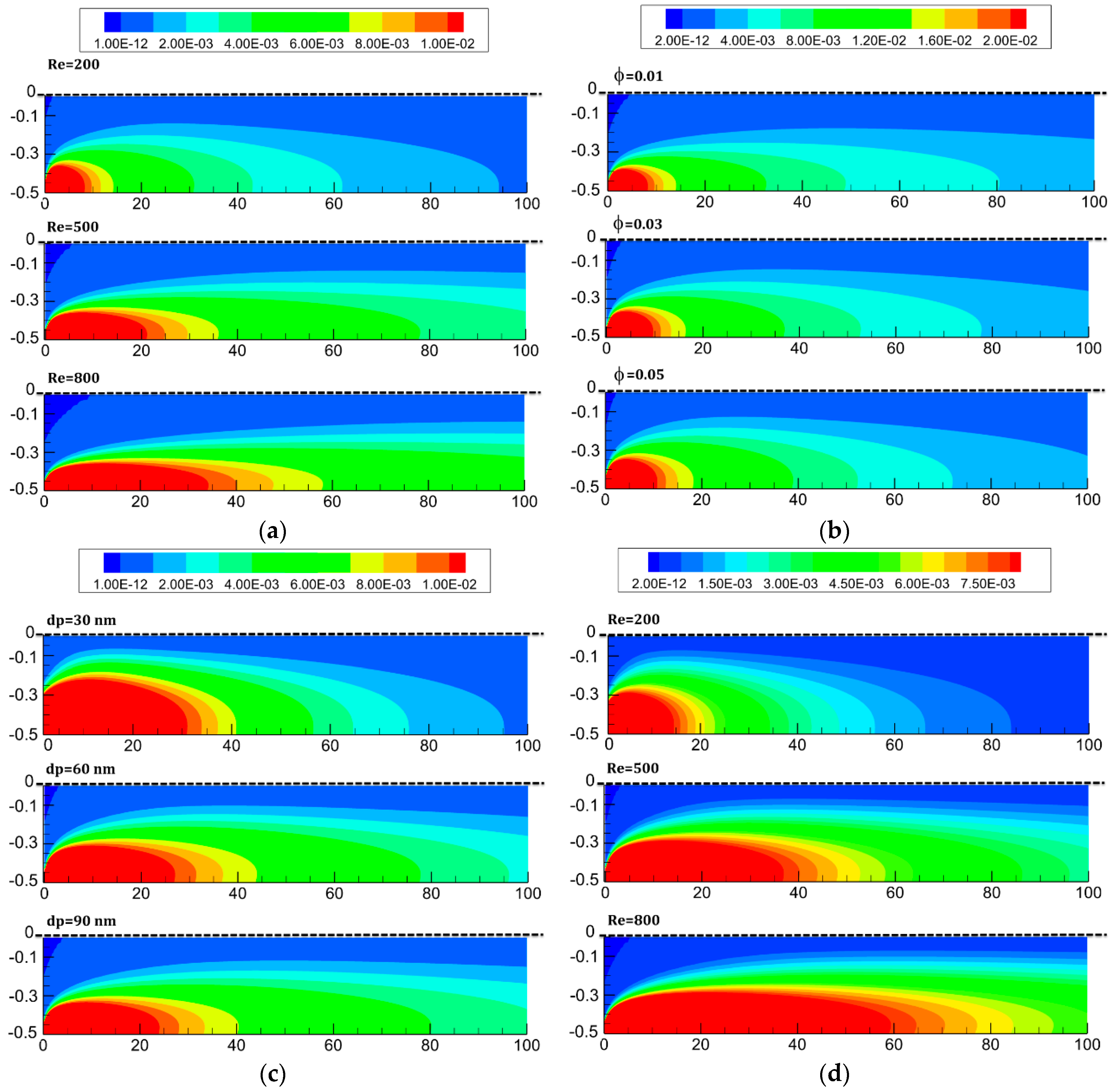
- The total entropy generation for nanofluid increases with increase in the Reynolds number and solid volume fraction. These augmentations are in the vicinity of 175% and 30% for 200 < Re < 800 and 0.01 < ϕ < 0.05, respectively.
- The total entropy generation decreases with increase in the nanoparticles diameter. This reduction is in the vicinity of 32% for 30 < dp < 90.
- The magnitude of total entropy generation, which increases with increase in the Reynolds number, is much higher for pure fluid rather than the nanofluid.
- The change in nanoparticles diameter has negligible effect on the entropy generation rate for low values of the Reynolds number.
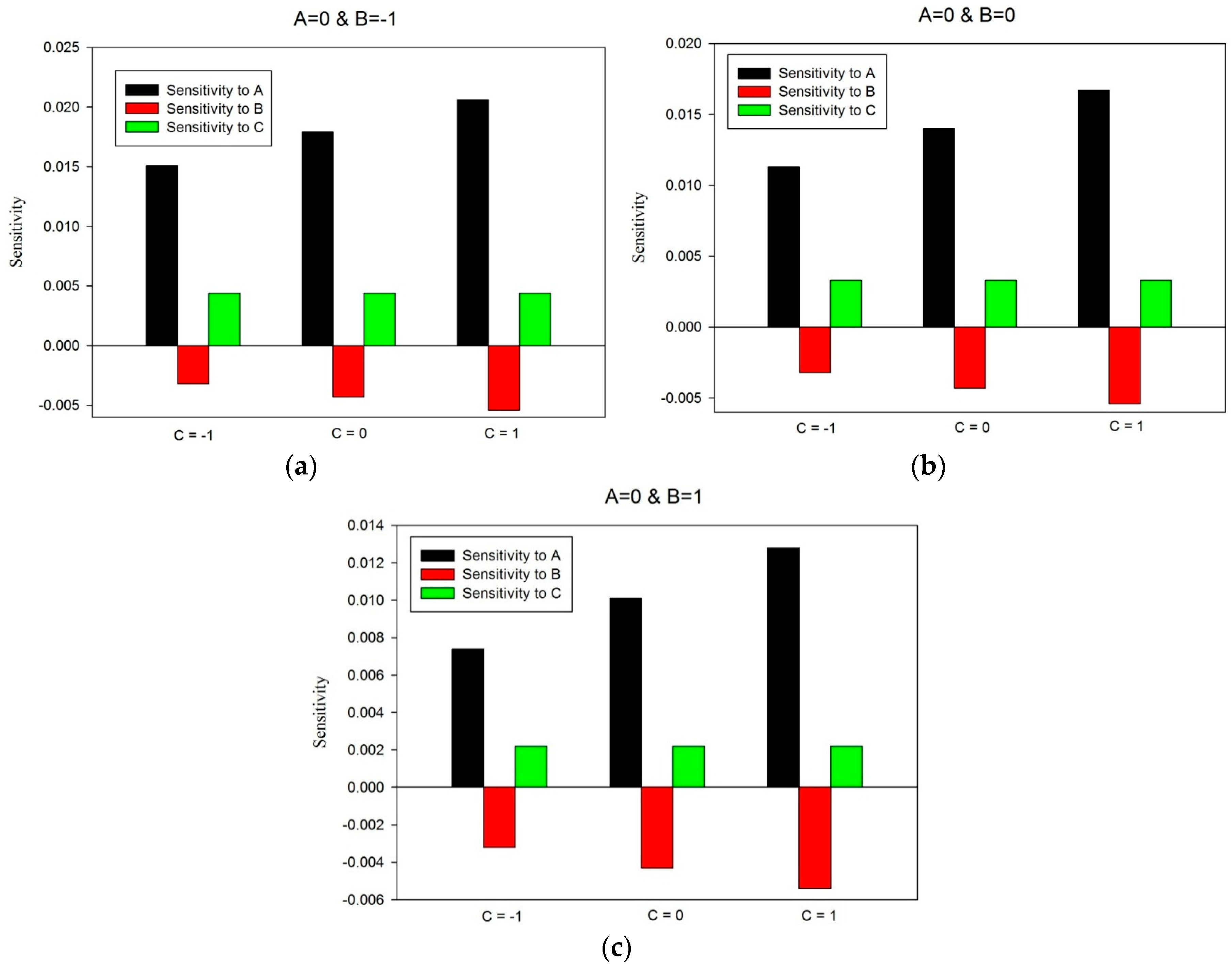
- The total entropy generation is more sensitive to the Reynolds number rather than the nanoparticles diameter or solid volume fraction.
- The sensitivities of the total entropy generation to the Reynolds number and nanoparticles diameter increase with increase in the solid volume fraction.
- The sensitivities of the total entropy generation to the Reynolds number and the solid volume fraction decrease with increase in nanoparticles diameter.
Author Contributions
Conflicts of Interest
Nomenclature
| a | number of factors (-) |
| ANOVA | analysis of variance (-) |
| Kb | Boltzmann constant (-) |
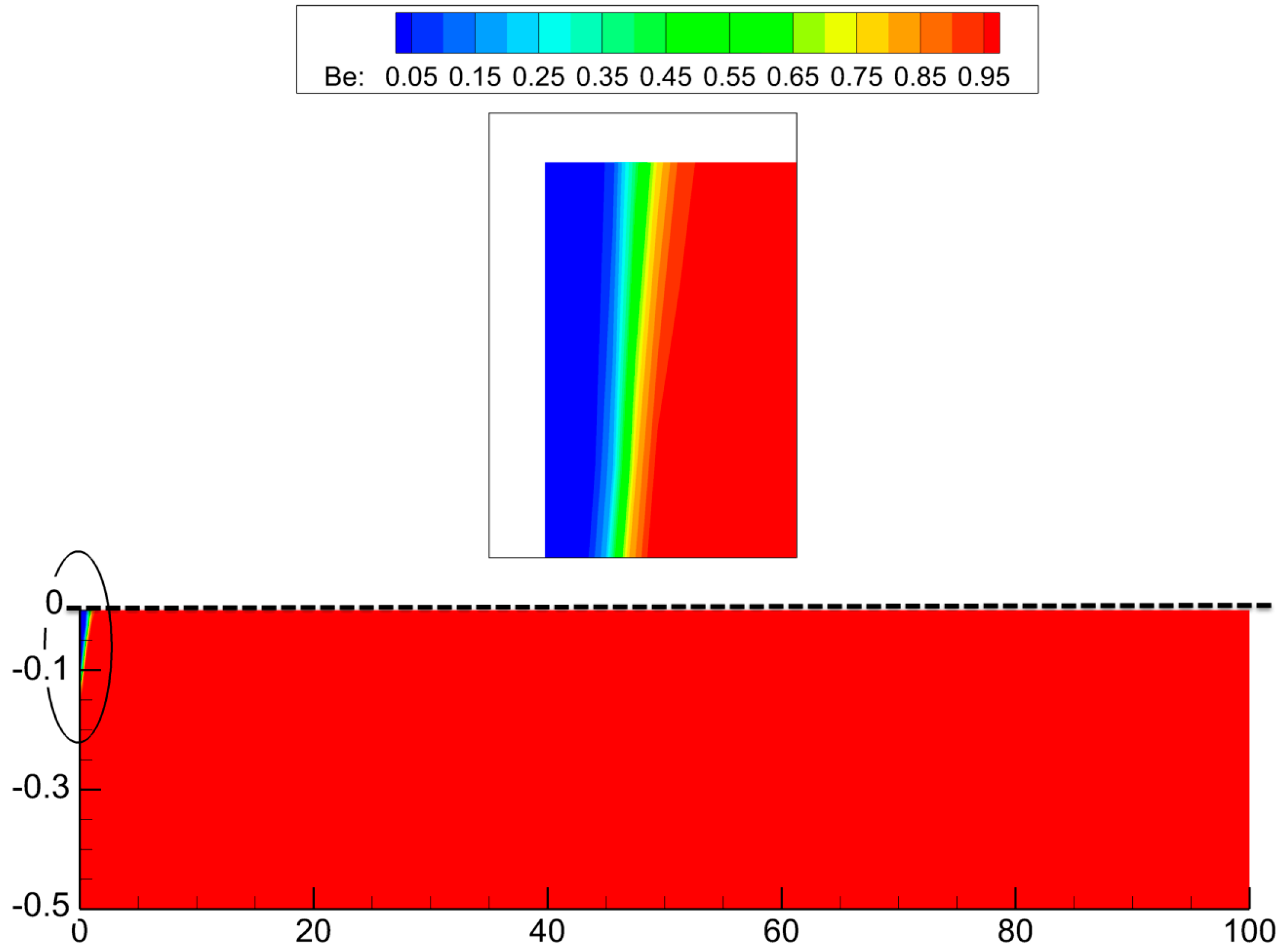
| Be | Bejan number (-) |
| b | number of center points (-) |
| C | specific heat at constant pressure (J·kg−1·K−1) |
| CCD | central composite design (-) |
| CCF | central composite face centered (-) |
| D | half of the channel gap (m) |
| df | molecular diameter of base fluid (nm) |
| dp | nanoparticle diameter (nm) |
| DOE | design of experiments (-) |
heat transfer coefficient (W·m−2·K−1) | |
thermal conductivity (W·m−1·K−1) | |
| L | length of the channel (m) |
| lBF | mean free path of water (-) |
| Ng | dimensionless local volumetric entropy generation rate (-) |
| Nt | dimensionless total entropy generation rate (-) |
pressure (Pa) | |
| Pe | Peclet number (Re×Pr) |
| Pr | Prandtl number () |
| Re | Reynolds number (ρU∞Dµ−1) |
| Res | response (-) |
| RSM | response surface methodology (-) |
entropy generation rate (W·m−3·K−1) | |
temperature (K) | |
velocity component in x and y directions, respectively (m·s−1) | |
| x, y | rectangular coordinates components (m) |
Greek Symbols
thermal diffusivity of fluid (m2·s−1) | |
dynamic viscosity (kg·m−1·s−1) | |
kinematic viscosity (m2·s−1) | |
density of the fluid (kg·m−3) | |
| ϕ | solid volume fraction (-) |
| δ | distance between particles (nm) |
| ∞ | free stream (-) |
Subscripts/Superscripts
| B | Brownian (-) |
| eff | effective |
| f | fluid |
| P | particle-pressure (-) |
| s | solid |
| w | wall |
References
- Santra, A.K.; Sen, S.; Chakraborty, N. Study of heat transfer due to laminar flow of copper–water nanofluid through two isothermally heated parallel plates. Int. J. Therm. Sci. 2009, 48, 391–400. [Google Scholar] [CrossRef]
- Radisi, A.; Ghasemi, B.; Aminossadati, S.M. A numerical study on the forced convection of laminar nanofluid in a microchannel with both slip and no-slip conditions. Numer. Heat Transf. 2011, 59, 114–129. [Google Scholar]
- Bianco, V.; Manca, O.; Nardini, S. Performance analysis of turbulent convection heat transfer of Al2O3 water-nanofluid in circular tubes at constant wall temperature. Energy 2014, 77, 403–413. [Google Scholar] [CrossRef]
- Heyhat, M.M.; Kowsary, F.; Rashidi, A.M.; Momenpour, M.H.; Amrollahi, A. Experimental investigation of laminar convective heat transfer and pressure drop of water-based Al2O3 nanofluids in fully developed flow regime. Exp. Therm. Fluid Sci. 2013, 44, 483–489. [Google Scholar] [CrossRef]
- Mahian, O.; Kianifar, A.; Kleinstreuer, C.; Al-Nimr, M.A.; Pop, I.; Wongwises, S.; Sahin, A.Z. A review of entropy generation in nanofluid flow. Int. J. Heat Mass Transf. 2013, 65, 514–532. [Google Scholar] [CrossRef]
- Malvandi, A.; Ganji, D.D.; Hedayati, F.; Rad, E.Y. An analytical study on entropy generation of nanofluids over a flat plate. Alex. Eng. J. 2013, 52, 595–604. [Google Scholar] [CrossRef]
- Khaleduzzaman, S.S.; Sohel, M.R.; Saidur, R.; Mahbubu, I.M.; Shahrul, I.M.; Akash, B.A.; Selvaraj, J. Energy and exergy analysis of alumina–water nanofluid for an electronic liquid cooling system. Int. Commun. Heat Mass Transf. 2014, 57, 118–127. [Google Scholar] [CrossRef]
- Khairul, M.A.; Mahbubul, I.M.; Saidur, R.; Hepbasli, A.; Hossain, A. Heat transfer performance and exergy analyses of a corrugated plate heat exchanger using metal oxide nanofluids. Int. Commun. Heat Mass Transf. 2014, 50, 8–14. [Google Scholar] [CrossRef]
- Mahmud, S.; Fraser, R.A. Thermodynamic analysis of flow and heat transfer inside channel with two parallel plates. Int. J. Heat Mass Transf. 2002, 2, 140–146. [Google Scholar] [CrossRef]
- Bianco, V.; Manca, O.; Nardini, S. Second law analysis of Al2O3-Water nanofluid turbulent forced convection in a circular cross section tube with constant wall temperature. Adv. Mech. Eng. 2013, 5, 920278. [Google Scholar] [CrossRef]
- Mah, W.H.; Hung, Y.M.; Guo, N. Entropy generation of viscous dissipative nanofluid flow in microchannels. Int. J. Heat Mass Transf. 2012, 55, 4169–4182. [Google Scholar] [CrossRef]
- Hajialigol, W.; Fattahi, A.; Haji-Ahmadi, M.; EbrahimQomi, M.; Kakoli, E. MHD mixed convection and entropy generation in a 3-D microchannel using Al2O3-water nanofluid. J. Taiwan Inst. Chem. Eng. 2015, 46, 30–42. [Google Scholar] [CrossRef]
- Korukcu, M.O. 2D temperature analysis of energy and exergy characteristics of laminar steady flow across a square cylinder under strong blockage. Entropy 2015, 17, 3124–3151. [Google Scholar] [CrossRef]
- Rashidi, S.; Bovand, M.; Esfahani, J.A. Heat transfer enhancement and pressure drop penalty in porous solar heat exchangers: A sensitivity analysis. Energy Convers. Manag. 2015, 103, 726–738. [Google Scholar] [CrossRef]
- Rashidi, S.; Bovand, M.; Esfahani, J.A. Structural optimization of nanofluid flow around an equilateral triangular obstacle. Energy 2015, 88, 385–398. [Google Scholar] [CrossRef]
- Rashidi, S.; Bovand, M.; Esfahani, J.A.; Ahmadi, G. Discrete particle model for convective Al2O3-water nanofluid around a triangular obstacle. Appl. Therm. Eng. 2016, in press. [Google Scholar]
- Breuer, M.; Bernsdorf, J.; Zeiser, T.; Durst, F. Accurate computations of the laminar flow past a square cylinder based on two different methods: Lattice-Boltzmann and finite-volume. Int. J. Heat Fluid Flow 2000, 21, 186–196. [Google Scholar] [CrossRef]
- Valipour, M.S.; Masoodi, R.; Rashidi, S.; Bovand, M.; Mirhosseini, M. A numerical study of convection around a square porous cylinder using Al2O3-H2O Nanofluid. Therm. Sci. 2014, 18, 1305–1314. [Google Scholar] [CrossRef]
- Bovand, M.; Rashidi, S.; Esfahani, J.A. Enhancement of heat transfer by nanofluids and orientations of the equilateral triangular obstacle. Energy Convers. Manag. 2015, 97, 212–223. [Google Scholar] [CrossRef]
- Zhou, S.Q.; Ni, R. Measurement of the specific heat capacity of water-based Al2O3 nanofluid. Appl. Phys. Lett. 2008, 92, 093–123. [Google Scholar] [CrossRef]
- Masoumi, N.; Sohrabi, N.; Behzadmehr, A. A new model for calculating the effective viscosity of nanofluids. J. Appl. Phys. D 2009, 42, 055501. [Google Scholar] [CrossRef]
- Rashidi, S.; Bovand, M.; Esfahani, J.A. Opposition of Magnetohydrodynamic and Al2O3-water nanofluid flow around a vertex facing triangular obstacle. J. Mol. Liq. 2016, 215, 276–284. [Google Scholar] [CrossRef]
- Chon, C.H.; Kihm, K.D.; Lee, S.P.; Choi, S.U. Empirical correlation finding the role of temperature and particle size for nanofluid (Al2O3) thermal conductivity enhancement. Appl. Phys. Lett. 2005, 87, 153107. [Google Scholar] [CrossRef]
- Bejan, A. A study of entropy generation in fundamental convective heat transfer. J. Heat Transf. 1979, 101, 718–729. [Google Scholar] [CrossRef]
- Esfahani, J.A.; Shahabi, P.B. Effect of non-uniform heating on entropy generation for the laminar developing pipe flow of a high Prandtl number fluid. Energy Convers. Manag. 2010, 51, 2087–2097. [Google Scholar] [CrossRef]
- Patankar, S. Numerical Heat Transfer and Fluid Flow; CRC Press: Boca Raton, FL, USA, 1980. [Google Scholar]
- Box, G.E.P.; Wilson, K.B. On the experimental attainment of optimum conditions. J. R. Stat. Soc. Ser. B 1951, 13, 1–45. [Google Scholar]
- Montgomery, D.C. Design and Analysis of Experiments; Wiley: Hoboken, NJ, USA, 1996. [Google Scholar]
- Bovand, M.; Valipour, M.S.; Dincer, K.; Eiamsa-ard, S. Application of Response Surface Methodology to optimization of a standard Ranque–Hilsch vortex tube refrigerator. Appl. Therm. Eng. 2014, 67, 545–553. [Google Scholar] [CrossRef]
- Yarmand, H.; Ahmadi, G.; Gharehkhani, S.; Kazi, S.N.; Safaei, M.R.; Sadat-Alehashem, M.; Mahat, A.B. Entropy generation during turbulent flow of zirconia-water and other nanofluids in a square cross section tube with a constant heat flux. Entropy 2014, 16, 6116–6132. [Google Scholar] [CrossRef]
© 2016 by the authors; licensee MDPI, Basel, Switzerland. This article is an open access article distributed under the terms and conditions of the Creative Commons by Attribution (CC-BY) license (http://creativecommons.org/licenses/by/4.0/).
Share and Cite
Darbari, B.; Rashidi, S.; Abolfazli Esfahani, J. Sensitivity Analysis of Entropy Generation in Nanofluid Flow inside a Channel by Response Surface Methodology. Entropy 2016, 18, 52. https://doi.org/10.3390/e18020052
Darbari B, Rashidi S, Abolfazli Esfahani J. Sensitivity Analysis of Entropy Generation in Nanofluid Flow inside a Channel by Response Surface Methodology. Entropy. 2016; 18(2):52. https://doi.org/10.3390/e18020052
Chicago/Turabian StyleDarbari, Bijan, Saman Rashidi, and Javad Abolfazli Esfahani. 2016. "Sensitivity Analysis of Entropy Generation in Nanofluid Flow inside a Channel by Response Surface Methodology" Entropy 18, no. 2: 52. https://doi.org/10.3390/e18020052