
Analysis of the Complexity Entropy and Chaos Control of the Bullwhip Effect Considering Price of Evolutionary Game between Two Retailers


Abstract
:1. Introduction
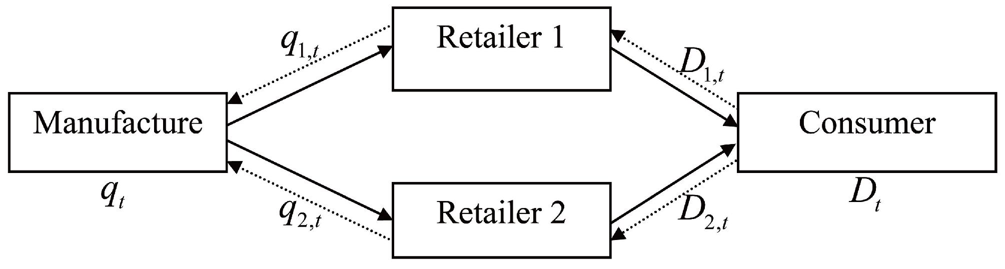
2. Price Game Model
2.1. Model Description
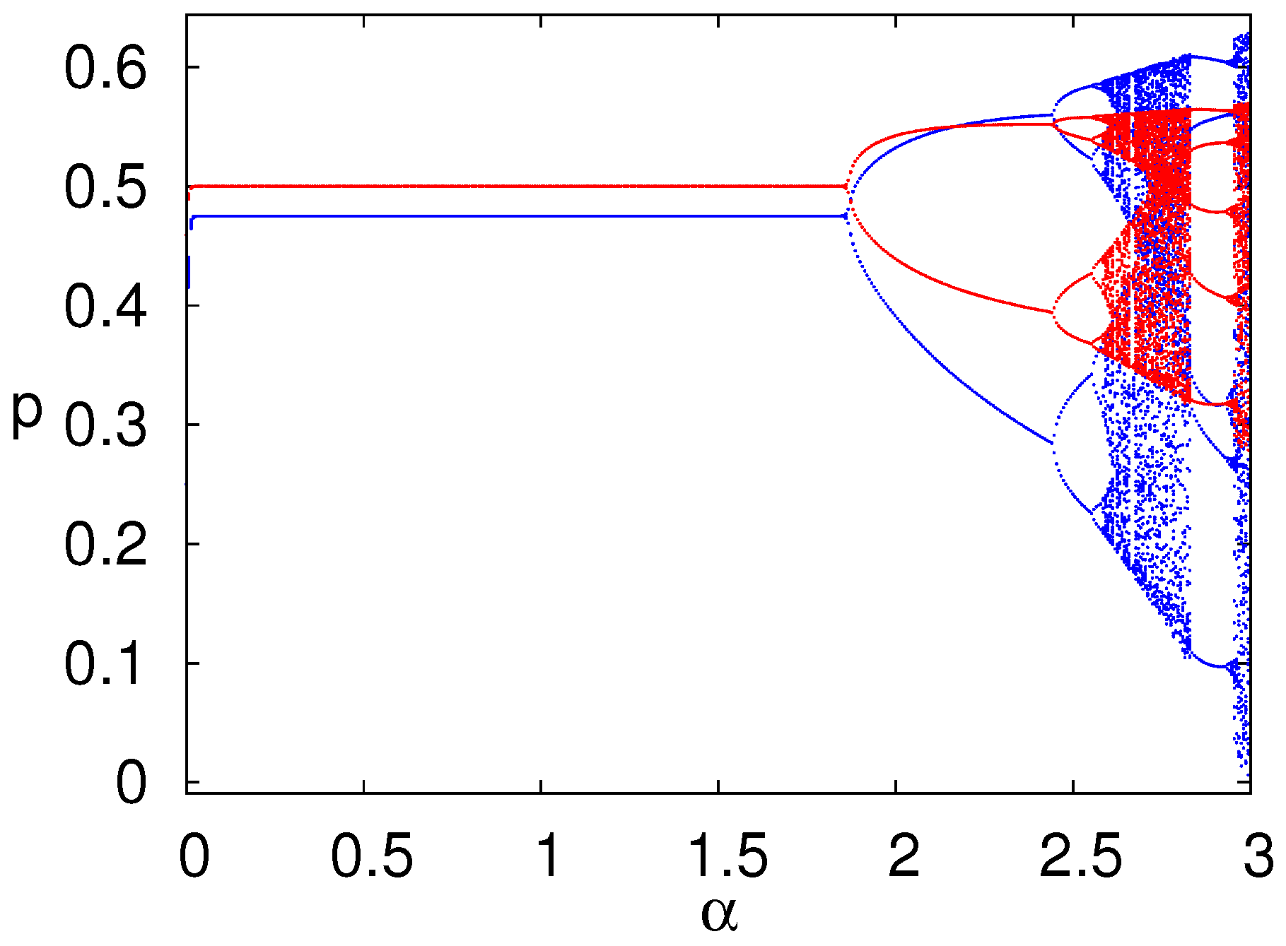
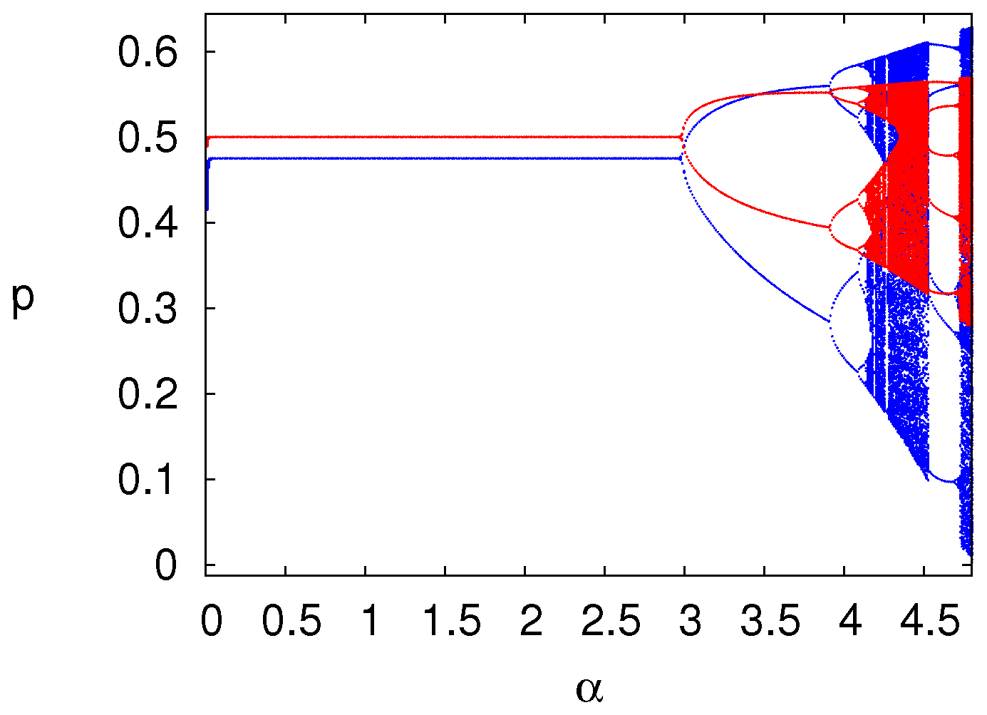
2.2. The Dynamics of the Price Game Model
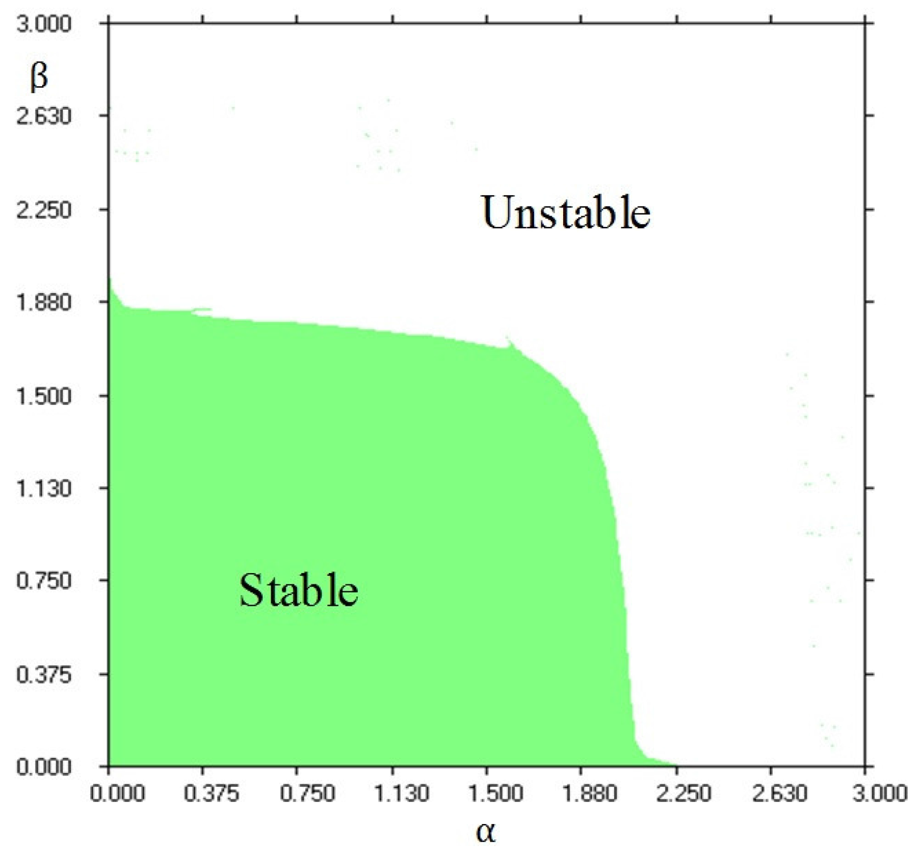
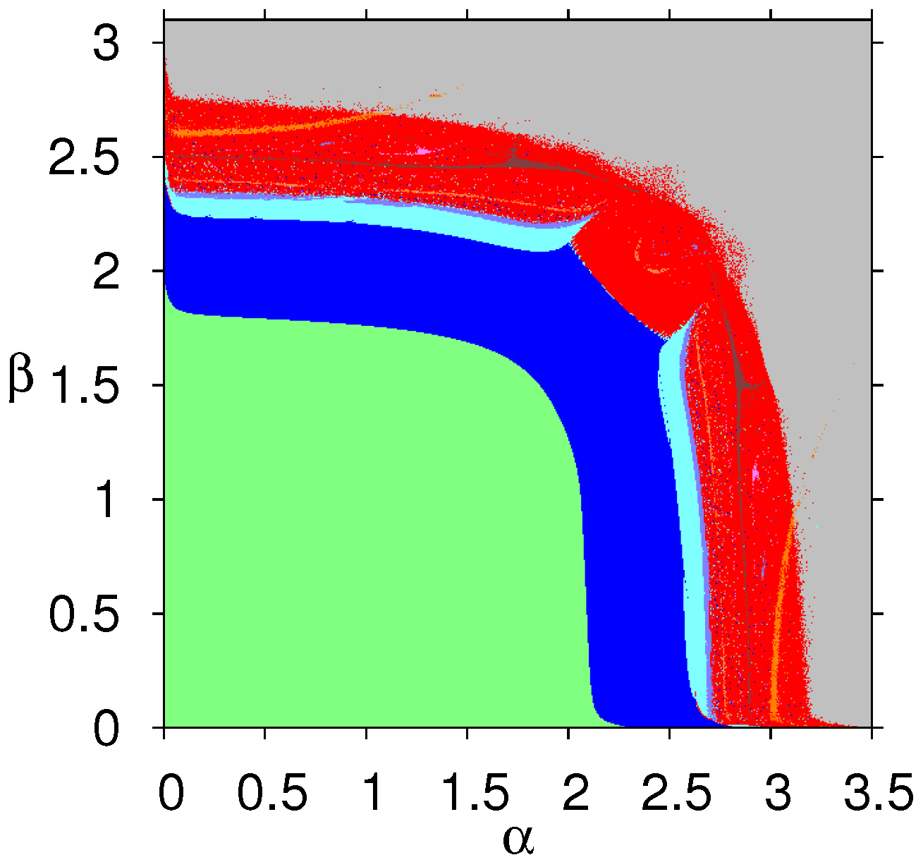
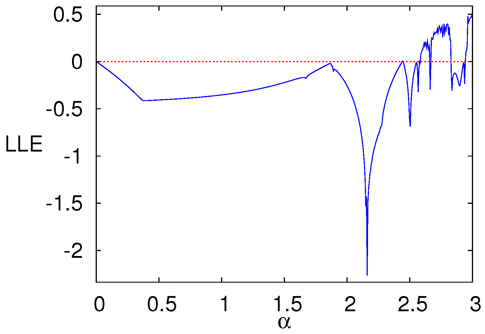
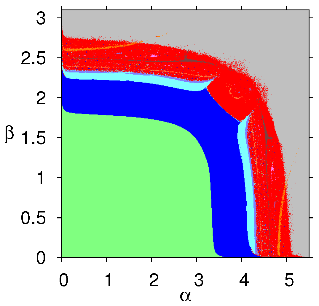
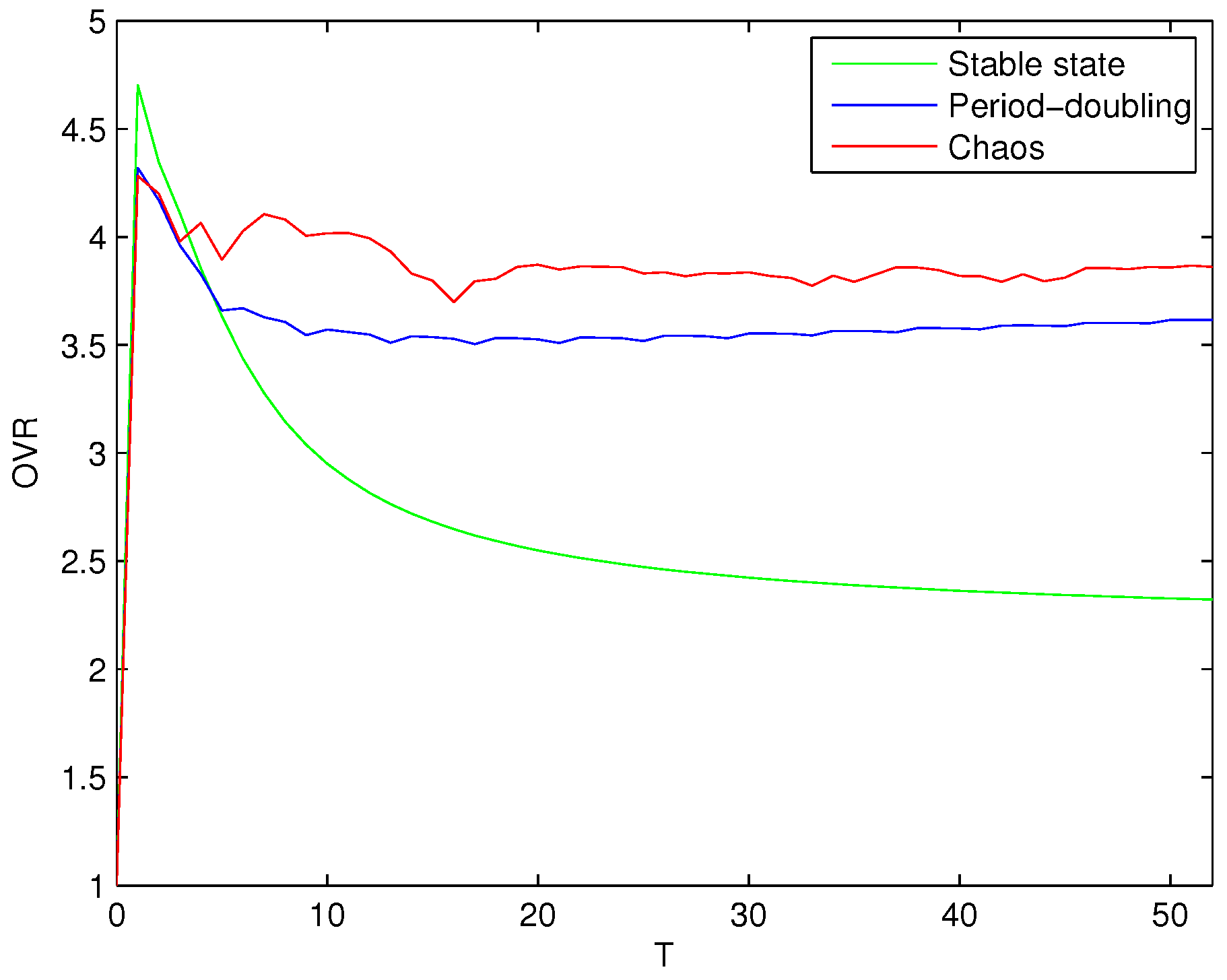
2.3. Experimental Design, Numerical Result and Discussion
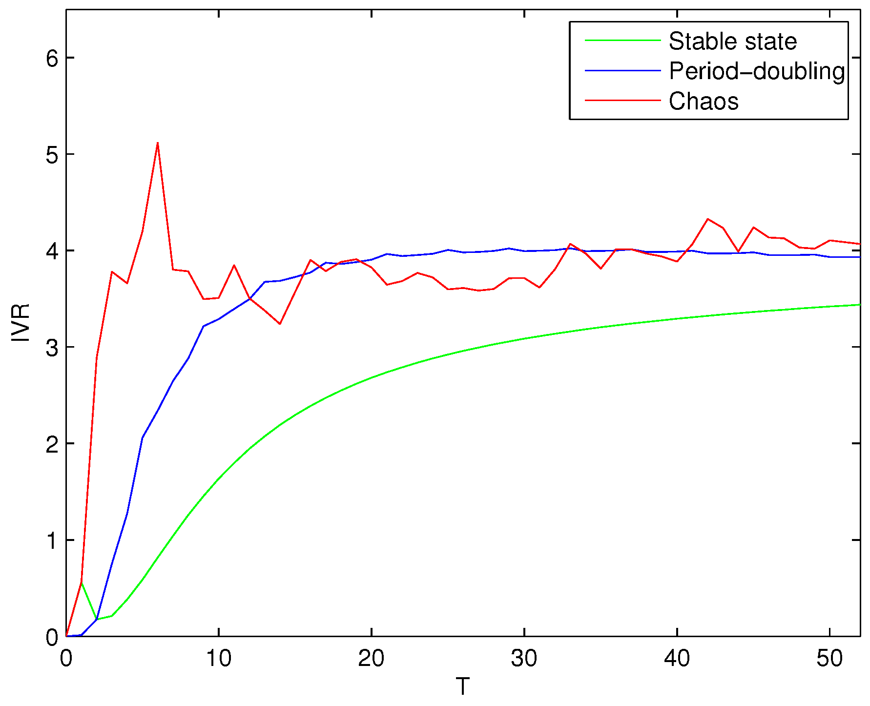
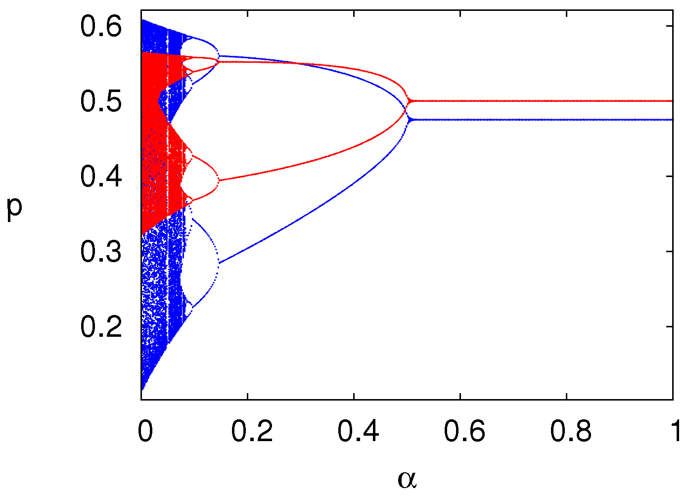
- (a)
- Stable state:
- (b)
- Period doubling:
- (c)
- Chaos:
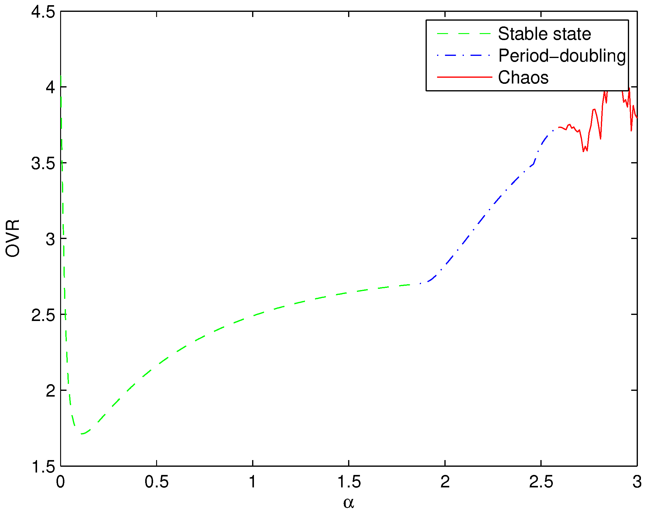
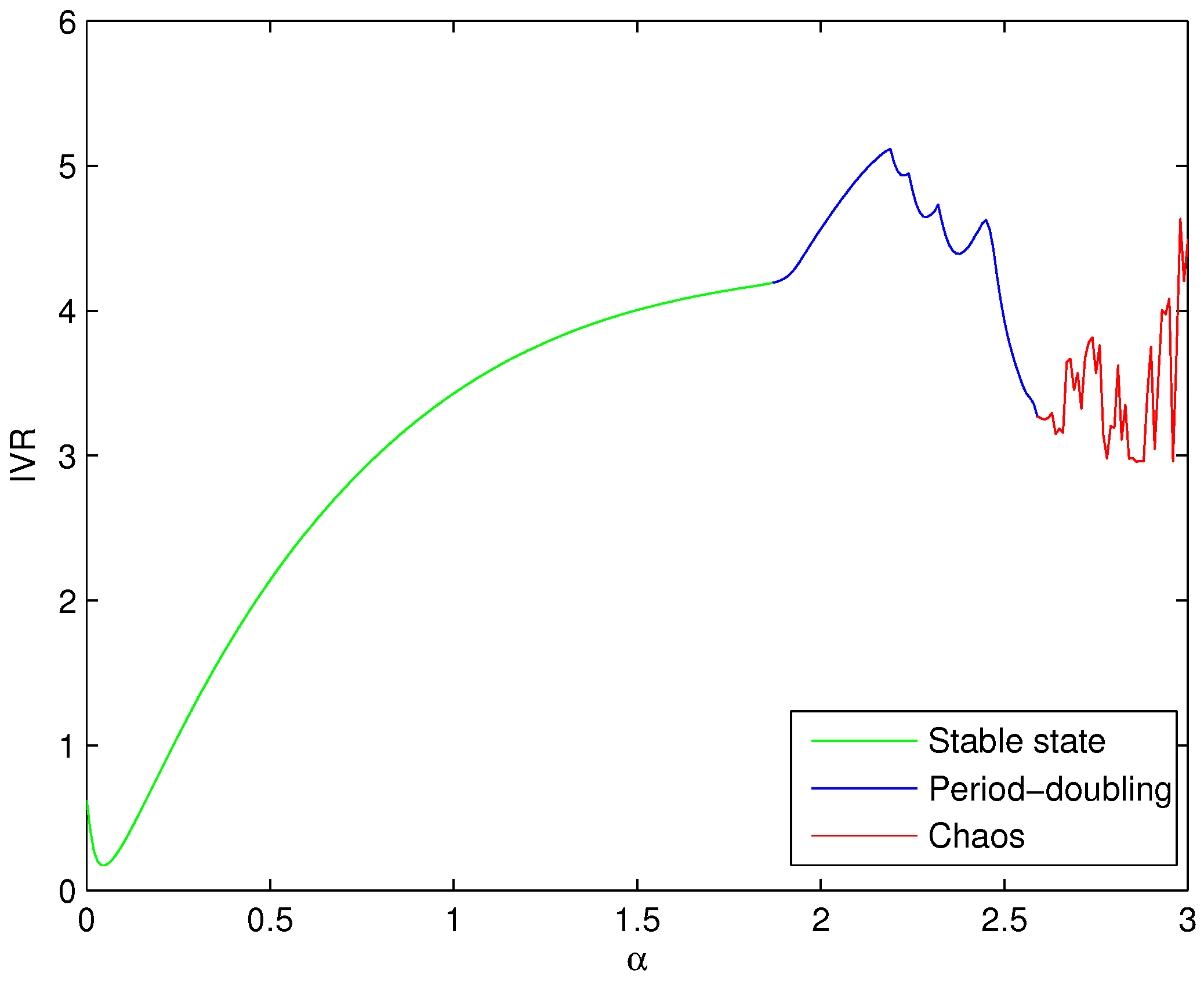
- (a)
- The lead-time of two retailers:
- (b)
- The safety stock factor:
- (c)
- The demand smoothing index:
- (d)
- The time length of numerical experiments:
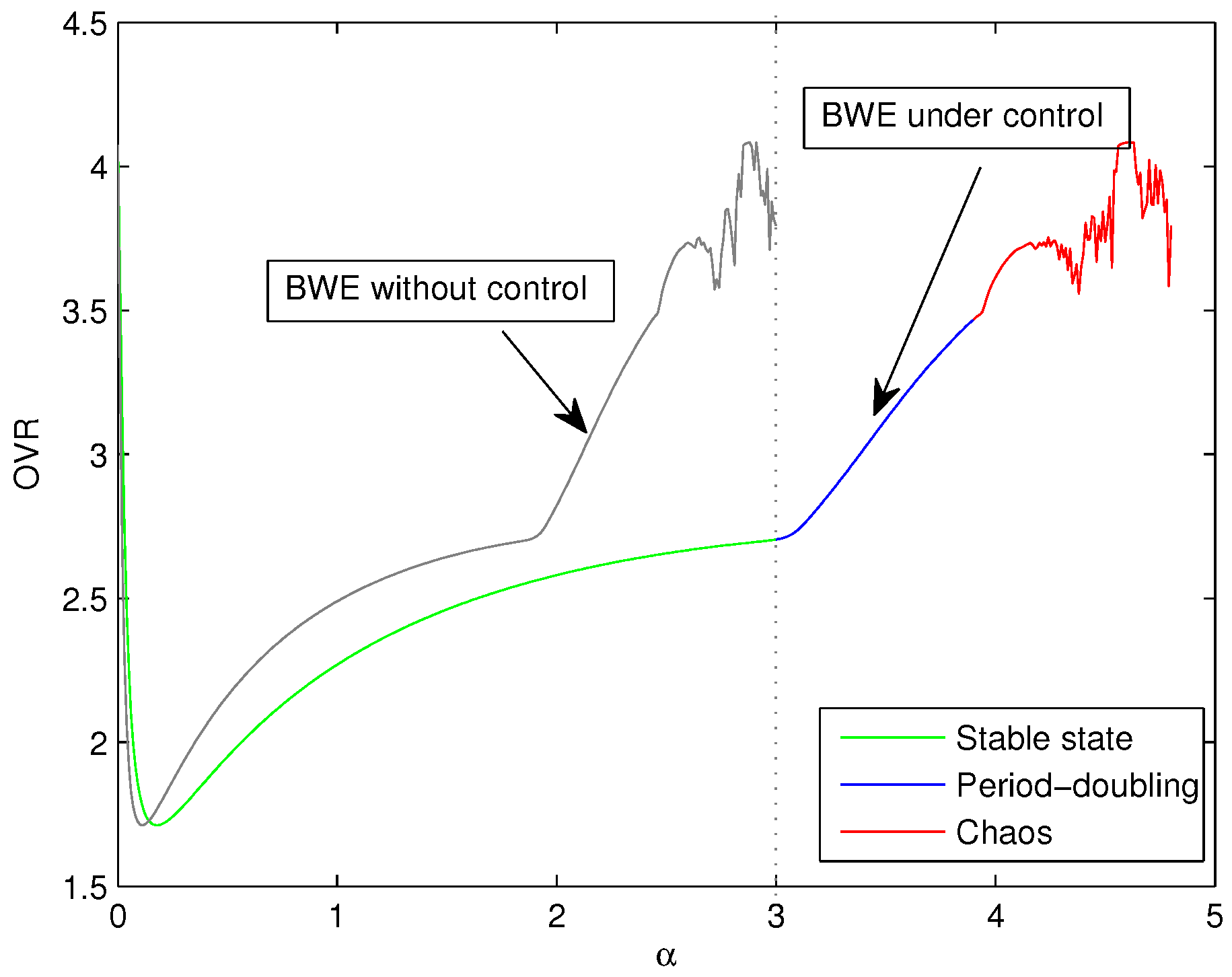
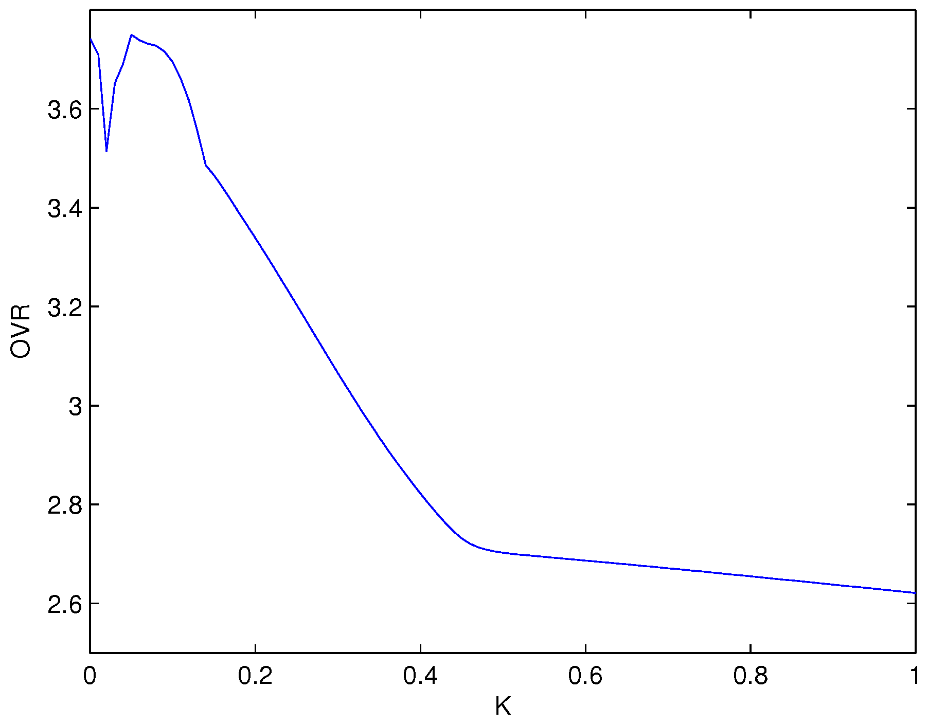
3. The Mitigation of the Bullwhip Effect by Chaos Control
4. Conclusions
Acknowledgments
Author Contributions
Conflicts of Interest
Appendix A. The Proof of Proposition
References
- Forrester, J.W. Industrial Dynamics; MIT Press: Cambridge, MA, USA, 1961. [Google Scholar]
- Sterman, J.D. Modeling managerial behavior: Misperceptions of feedback in a dynamic decision making experiment. Manag. Sci. 1989, 35, 321–339. [Google Scholar] [CrossRef]
- Lee, H.L.; Padmanabhan, P.; Whang, S. Information distortion in a supply chain: The bullwhip effect. Manag. Sci. 1997, 43, 546–558. [Google Scholar] [CrossRef]
- Chen, F.; Drezner, Z.; Ryan, J.K.; Simchi-Levi, D. Quantifying the bullwhip effect in a simple supply chain. Manag. Sci. 2000, 46, 436–443. [Google Scholar] [CrossRef]
- Chen, F.; Drezner, Z.; Ryan, J.K.; Simchi-Levi, D. The impact of exponential smoothing forecasts on the bullwhip effect. Naval Res. Logist. 2000, 47, 269–286. [Google Scholar] [CrossRef]
- Zhang, X. The impact of forecasting methods on the bullwhip effect. Int. J. Prod. Econ. 2004, 88, 15–27. [Google Scholar] [CrossRef]
- Luong, H.T. Measure of bullwhip effect in supply chains with autoregressive demand process. Eur. J. Oper. Res. 2007, 180, 1086–1097. [Google Scholar] [CrossRef]
- Agrawal, S.; Sengupta, R.N.; Shanker, K. Impact of information sharing and lead time on bullwhip effect and on-hand inventory. Eur. J. Oper. Res. 2009, 192, 576–593. [Google Scholar] [CrossRef]
- Chatfield, D.C.; Kim, J.G.; Harrison, T.P.; Hayya, J.C. The bullwhip effect-impact of stochastic lead time, information quality, and information sharing: A simulation study. Prod. Oper. Manag. 2004, 13, 340–353. [Google Scholar] [CrossRef]
- Cannella, S.; Ciancimino, E. On the bullwhip avoidance phase: Supply chain collaboration and order smoothing. Int. J. Prod. Res. 2010, 48, 6739–6776. [Google Scholar] [CrossRef]
- Cannella, S.; Ciancimino, E.; Framinan, J.M. Inventory policies and information sharing in multi-echelon supply chains. Prod. Plan. Control 2011, 22, 649–659. [Google Scholar] [CrossRef]
- Cannella, S.; Framinan, J.M.; Barbosa-Povoa, A. An IT-enabled supply chain model: A simulation study. Int. J. Syst. Sci. 2014, 45, 2327–2341. [Google Scholar] [CrossRef]
- Cannella, S.; Bruccoleri, M.; Framinan, J.M. Closed-loop supply chains: What reverse logistics factors influence performance? Int. J. Prod. Econ. 2016, 175, 35–49. [Google Scholar] [CrossRef]
- Cannella, S.; Barbosa-Povoa, A.P.; Framinan, J.M.; Relvas, S. Metrics for bullwhip effect analysis. J. Oper. Res. Soc. 2013, 64, 1–16. [Google Scholar] [CrossRef]
- Trapero, J.R.; Kourentzes, N.; Fildes, R. Impact of information exchange on supplier forecasting performance. Omega 2012, 40, 738–747. [Google Scholar] [CrossRef] [Green Version]
- Ciancimino, E.; Cannella, S.; Bruccoleri, M.; Framinan, J.M. On the bullwhip avoidance phase: The synchronised supply chain. Eur. J. Oper. Res. 2012, 221, 49–63. [Google Scholar] [CrossRef] [Green Version]
- Dominguez, R.; Cannella, S.; Framinan, J.M. On bullwhip-limiting strategies in divergent supply chain networks. Comput. Ind. Eng. 2014, 73, 85–95. [Google Scholar] [CrossRef]
- Dominguez, R.; Cannella, S.; Framinan, J.M. The impact of the supply chain structure on bullwhip effect. Appl. Math. Model. 2015, 39, 7309–7325. [Google Scholar] [CrossRef]
- Duc, T.T.; Luong, H.T.; Kim, Y.D. A measure of bullwhip effect in supply chains with a mixed autoregressive-moving average demand process. Eur. J. Oper. Res. 2008, 187, 243–256. [Google Scholar] [CrossRef]
- Ma, Y.; Wang, N.; Che, A.; Huang, Y.; Xu, J. The bullwhip effect under different information-sharing settings: A perspective on price-sensitive demand that incorporates price dynamics. Int. J. Prod. Res. 2013, 51, 3085–3116. [Google Scholar] [CrossRef] [Green Version]
- Wang, N.; Lu, J.; Feng, G.; Ma, Y.; Liang, H. The bullwhip effect on inventory under different information sharing settings based on price-sensitive demand. Int. J. Prod. Res. 2016, 54, 4043–4064. [Google Scholar] [CrossRef]
- Ma, Y.; Wang, N.; He, Z.; Lu, J.; Liang, H. Analysis of the bullwhip effect in two parallel supply chains with interacting price-sensitive demands. Eur. J. Oper. Res. 2015, 243, 815–825. [Google Scholar] [CrossRef]
- Larsen, E.R.; Morecroft, J.D.W.; Thomsen, J.S. Complex behaviour in a production-distribution model. Eur. J. Oper. Res. 1999, 119, 61–74. [Google Scholar] [CrossRef]
- Hwarng, H.B.; Xie, N. Understanding supply chain dynamics: A chaos perspective. Eur. J. Oper. Res. 2008, 184, 1163–1178. [Google Scholar] [CrossRef]
- Hwarng, H.B.; Yuan, X. Interpreting supply chain dynamics: A quasi-chaos perspective. Eur. J. Oper. Res. 2014, 233, 566–579. [Google Scholar] [CrossRef]
- Mosekilde, E.; Laugesen, J.L. Nonlinear dynamic phenomena in the beer model. Syst. Dyn. Rev. 2007, 23, 229–252. [Google Scholar] [CrossRef]
- Wang, X.; Disney, S.M.; Wang, J. Stability analysis of constrained inventory systems with transportation delay. Eur. J. Oper. Res. 2012, 223, 86–95. [Google Scholar] [CrossRef]
- Wang, X.; Disney, S.M.; Wang, J. Exploring the oscillatory dynamics of a forbidden returns inventory system. Int. J. Prod. Econ. 2014, 147, 3–12. [Google Scholar] [CrossRef]
- Gao, B.; Wu, C.; Wu, Y.; Tang, Y. Expected Utility and Entropy-Based Decision-Making Model for Large Consumers in the Smart Grid. Entropy 2015, 17, 6560–6575. [Google Scholar] [CrossRef]
- Zou, Y.; Yu, L.; He, K. Wavelet Entropy Based Analysis and Forecasting of Crude Oil Price Dynamics. Entropy 2015, 17, 7167–7184. [Google Scholar] [CrossRef]
- Ma, J.; Si, F. Complex Dynamics of a Continuous Bertrand Duopoly Game Model with Two-Stage Delay. Entropy 2016, 18, 266. [Google Scholar] [CrossRef]
- Disney, S.M.; Towill, D.R. The effect of vendor managed inventory (VMI) dynamics on the Bullwhip Effect in supply chains. Int. J. Prod. Econ. 2003, 85, 199–215. [Google Scholar] [CrossRef]
- Costantino, F.; Di Gravio, G.; Shaban, A.; Tronci, M. The impact of information sharing on ordering policies to improve supply chain performances. Comput. Ind. Eng. 2015, 82, 127–142. [Google Scholar] [CrossRef]
- Xie, L.; Ma, J. Study the complexity and control of the recycling-supply chain of China’s color TVs market based on the government subsidy. Commun. Nonlinear Sci. Numer. Simul. 2016, 38, 102–116. [Google Scholar] [CrossRef]
- Zhang, J.; Ma, J. Research on the price game model for four oligarchs with different decision rules and its chaos control. Nonlinear Dyn. 2012, 70, 323–334. [Google Scholar] [CrossRef]


© 2016 by the authors; licensee MDPI, Basel, Switzerland. This article is an open access article distributed under the terms and conditions of the Creative Commons Attribution (CC-BY) license (http://creativecommons.org/licenses/by/4.0/).
Share and Cite
Ma, J.; Ma, X.; Lou, W. Analysis of the Complexity Entropy and Chaos Control of the Bullwhip Effect Considering Price of Evolutionary Game between Two Retailers. Entropy 2016, 18, 416. https://doi.org/10.3390/e18110416
Ma J, Ma X, Lou W. Analysis of the Complexity Entropy and Chaos Control of the Bullwhip Effect Considering Price of Evolutionary Game between Two Retailers. Entropy. 2016; 18(11):416. https://doi.org/10.3390/e18110416
Chicago/Turabian StyleMa, Junhai, Xiaogang Ma, and Wandong Lou. 2016. "Analysis of the Complexity Entropy and Chaos Control of the Bullwhip Effect Considering Price of Evolutionary Game between Two Retailers" Entropy 18, no. 11: 416. https://doi.org/10.3390/e18110416