
Multivariate Generalized Multiscale Entropy Analysis


Univ Angers, LARIS-Laboratoire Angevin de Recherche en Ingénierie des Systèmes, 62 avenue Notre-Dame du Lac, 49000 Angers, France
Entropy 2016, 18(11), 411; https://doi.org/10.3390/e18110411
Submission received: 22 September 2016
/
Revised: 2 November 2016
/
Accepted: 14 November 2016
/
Published: 17 November 2016
(This article belongs to the Special Issue Multivariate Entropy Measures and Their Applications)
Abstract
:Multiscale entropy (MSE) was introduced in the 2000s to quantify systems’ complexity. MSE relies on (i) a coarse-graining procedure to derive a set of time series representing the system dynamics on different time scales; (ii) the computation of the sample entropy for each coarse-grained time series. A refined composite MSE (rcMSE)—based on the same steps as MSE—also exists. Compared to MSE, rcMSE increases the accuracy of entropy estimation and reduces the probability of inducing undefined entropy for short time series. The multivariate versions of MSE (MMSE) and rcMSE (MrcMSE) have also been introduced. In the coarse-graining step used in MSE, rcMSE, MMSE, and MrcMSE, the mean value is used to derive representations of the original data at different resolutions. A generalization of MSE was recently published, using the computation of different moments in the coarse-graining procedure. However, so far, this generalization only exists for univariate signals. We therefore herein propose an extension of this generalized MSE to multivariate data. The multivariate generalized algorithms of MMSE and MrcMSE presented herein (MGMSE and MGrcMSE, respectively) are first analyzed through the processing of synthetic signals. We reveal that MGrcMSE shows better performance than MGMSE for short multivariate data. We then study the performance of MGrcMSE on two sets of short multivariate electroencephalograms (EEG) available in the public domain. We report that MGrcMSE may show better performance than MrcMSE in distinguishing different types of multivariate EEG data. MGrcMSE could therefore supplement MMSE or MrcMSE in the processing of multivariate datasets.
1. Introduction
Multiscale entropy (MSE) was proposed in the 2000s to quantify the degree of unpredictability of systems across multiple scales [1,2]. Its computation relies on two steps [1,2]: (i) a coarse-graining procedure to derive a set of time series representing the system dynamics on different time scales. The coarse-graining procedure for scale τ is obtained by averaging the samples of the time series inside consecutive but non-overlapping windows of length τ. The length of a coarse-grained time series at a scale factor τ is equal to , where N is the number of samples in the original signal. (ii) Computation of the sample entropy for each coarse-grained time series. Sample entropy is equal to the negative of the natural logarithm of the conditional probability that sequences close to each other for m consecutive data points will also be close to each other when one more point is added to each sequence [3].
Since its introduction, MSE has been used in a variety of applications [4]. However, to increase the accuracy of entropy estimation, and to reduce the probability of inducing undefined entropy for short time series, a refined composite multiscale entropy (rcMSE) has recently been proposed [5]. rcMSE is based on the same steps as MSE (see below).
Recently, Costa et al. reported a generalization of the MSE algorithm [6]: they proposed MSE, where n corresponds to the moment used to coarse-grain a time series. MSE uses the mean value (first moment) and corresponds to the standard MSE. In the generalized MSE algorithm, the second, third, or higher moment can be used in the non-overlapping segments of length τ [6]. Using MSE, it has been shown that human heartbeat volatility time series exhibit complex bursting behaviors over a wide range of time scales, and that multiscale complexity of the volatility degrades with aging and pathology [6].
MSE and its generalization are able to process univariate datasets only. For multivariate time series, individual time series are processed separately. This may be satisfactory only if the individual signals are statistically independent or at least uncorrelated. This is often not the case when real world signals from a given system are registered simultaneously. To overcome this shortcoming, the multivariate MSE (MMSE) and multivariate rcMSE (MrcMSE) have been proposed [7,8,9]. MMSE and MrcMSE are able to operate on any number of data channels, and provide a robust relative complexity measure for multivariate data [7,8,9]. However, MMSE and MrcMSE only consider coarse-grained time series from the first-order moment of the samples contained inside windows.
In this work, we extend the MMSE and MrcMSE algorithms to a more general case. To this end, we introduce the multivariate generalized MSE (MGMSE) and the multivariate generalized rcMSE (MGrcMSE), and evaluate their performance on both synthetic and real-world multivariate processes.
2. Materials and Methods
2.1. Multiscale Entropy
As mentioned above, the MSE algorithm is composed of two steps [1,2]
- A coarse-graining procedure. For a monovariate discrete signal of length N , the coarse-grained time series is computed asFor scale one, the coarse-grained time series corresponds to the original signal. The length of the coarse-grained time series is . Coarse-graining can be seen as an averaging of the data inside a window of length τ (to reduce the high frequency components), followed by a downsampling of the averaged data by a factor τ [10]. Moreover, it has been reported that Equation (1) is similar to the use of a finite-impulse response (FIR) filter on the original time series x and to the downsampling of the filtered signal with a factor τ [11]. This FIR filter is a low-pass filter.
- Computation of the sample entropy for each coarse-grained time series. The sample entropy quantifies the regularity of finite length time series [3]. A low value for the sample entropy reflects a high degree of regularity, while a random signal has a relatively higher value of sample entropy. Sample entropy is a conditional probability measure that quantifies the likelihood that a sequence of m consecutive data points—that matches another sequence of the same length (match within a tolerance of r)—will still match the other sequence when their length is increased by one sample (sequences of length ); m therefore defines the length of the patterns that are compared to each other [3]. For a time series , the sample entropy is computed aswhere represents the total number of m-dimensional matched vector pairs, and represents the total number of -dimensional matched vector pairs. More precisely,withand is the number of vectors such that . In the definition of sample entropy, the distance d between two vectors is defined as the maximum absolute difference of their corresponding scalar components [3].
From Equation (2), MSE can be written as
where represents the total number of m-dimensional matched vector pairs, and is constructed from the coarse-grained time series at the scale factor τ. In the MSE algorithm, two patterns are considered similar if they are closer than a parameter r. The value of r is usually chosen as a percentage of the standard deviation of the signal under study. In the original algorithm of MSE proposed by Costa et al. (algorithm described above; [1,2]), the value of r is constant for all scale factors.
2.2. Refined Composite Multiscale Entropy
MSE has been used widely. However, because the coarse-graining procedure reduces the length of the time series, MSE may yield an inaccurate estimation of entropy or induce undefined entropy at large scales or for short time series. rcMSE has been proposed to overcome this drawback [5]. Compared to MSE, rcMSE increases the accuracy of entropy estimation and reduces the probability of inducing undefined entropy for short time series. For a monovariate discrete signal of length N , the rcMSE algorithm is based on the following steps [5]:
- For a scale factor τ, τ coarse-grained time series are generated. The k-th coarse-grained time series for a scale factor τ is defined as , where [12]
- For each scale factor τ, and for all τ coarse-grained time series, the number of matched vector pairs and is computed, where represents the total number of m-dimensional matched vector pairs and is computed from the k-th coarse-grained time series at a scale factor τ
- rcMSE is then defined as [5]
2.3. Multivariate (Refined Composite) Multiscale Entropy
MMSE, the extension of MSE to multivariate datasets—denoted as MGMSE in what follows—relies on the same steps as MSE [7,8]: a coarse-graining procedure and a sample entropy computation for each coarse-grained time series. Each of these two steps is adapted to multivariate data. Thus, for the coarse-graining procedure, temporal scales are defined by averaging a p-variate time series ( is the channel index and N is the number of samples in every channel) over time segments of increasing length. Thus, for a scale factor τ, a multi-channel coarse-grained time series is computed as (here the channel index l goes from 1 to p)
In the sample entropy computation step, the multivariate sample entropy (MSampEn) is used. The MSampEn algorithm is an extension of the univariate sample entropy [3]. In this case, the embedding dimension for the channel k of the multivariate data is noted as . The detailed MSampEn algorithm can be found in [7,8]. Briefly, for a tolerance level r, MSampEn is calculated as the negative of the natural logarithm of the conditional probability that two composite delay vectors close to each other in a m dimensional space will also be close to each other when the dimensionality is increased by one.
2.4. Multivariate Generalized (Refined Composite) Multiscale Entropy
In the multivariate extension of the generalized MSE (MGMSE) and generalized rcMSE (MGrcMSE) that we propose, the same steps as the ones of MMSE (resp. MrcMSE) are found, except in the coarse-graining procedure, where the averaging is replaced by the computation of the second moment (MGMSE and MGrcMSE) or by the computation of the third moment (MGMSE and MGrcMSE), and so on. MGMSE and MGrcMSE quantify the dynamics of the volatility over multiple time scales [6]. Thus, for MGMSE, the coarse-grained multivariate time series at scale factor τ is computed as
where corresponds to the mean of . MGMSE is determined as in Equation (9) where the computation of the variance is replaced by the computation of the skewness (similar steps are used to compute MGrcMSE and MGrcMSE, see Figure 1). From Equation (9), we observe that MGMSE and MGrcMSE are 0 for scale factor . In what follows, we will therefore concentrate on scale factors larger than 1 for MGMSE and MGrcMSE. For the same reason, we will concentrate on scale factors larger than 2 for MGMSE and MGrcMSE. Hereafter we will study MGMSE, MGrcMSE, MGMSE, and MGrcMSE on synthetic and real datasets.
2.5. Datasets Acquisition
The new algorithms that we propose were tested on synthetic signals, but also on two publicly available experimental biomedical datasets [13,14]. The first set consisted of five two-channel electroencephalogram (EEG) data (bivariate data) recorded at the left and right frontal cortex of male adult WAG/Rij rats. Each signal lasted 5 s and was digitized at 200 Hz. Each one was filtered between 1 and 100 Hz. More details on the acquisition procedure can be found in [15,16]. For this first set, data A correspond to a normal EEG, and data B, C, D, and E contain spike-wave discharges which are the landmark of epileptic activity. These spike-wave discharges are due to abnormal synchronization in an epileptic brain, even when there are no seizures [16]. The synchronization level differs between the data, as has been previously reported [16]. The length of each data segment was only 5 s (1000 samples), because this length was considered to be the largest one in which the signals containing spikes could be visually judged as stationary [15].
The second set of experimental biomedical data consisted of five (data A to E) two-channel EEG data (bivariate data) recorded in humans [17]. The segments processed thereafter were selected and cut out from continuous multichannel EEG recordings after visual inspection for artifacts (e.g., due to muscle activity or eye movements). In addition, the segments had to fulfill a stationarity criterion [17]. Data A and B are segments taken from surface EEG data recorded in healthy volunteers. Volunteers were relaxed in an awake state with eyes open (data A) and eyes closed (data B). Data C, D, and E are EEG from patients who had achieved complete seizure control after resection of one of the hippocampal formations, which was therefore correctly diagnosed to be the epileptogenic zone. Data C were recorded from the hippocampal formation of the opposite hemisphere of the brain, and data D were recorded from within the epileptogenic zone. Data C and D contain only activity measured during seizure-free intervals. Data E contain only seizure activity. The data were selected from all recording sites exhibiting ictal activity. All these data were recorded during 23.6 s with a sampling frequency of 173.61 Hz. They therefore contain 4097 samples. Further details on the acquisition can be found in [17].
3. Experimental Results and Discussion
3.1. Results for Synthetic Signals
We recall that noise time series are more complex than uncorrelated (white) noise time series due to long-range correlations of noise data [1]. Furthermore, a multivariate time series is considered more structurally complex than another if (for most of the scale factors) its multivariate entropy values are higher than those of the other time series. When the multivariate entropy values decrease with the scale factor, the data that are processed contain information only at the smallest scales. They are thus not structurally complex.
Moreover, multivariate data showing a constant entropy measure or a monotonic increase of entropy value with increasing scale factors are data presenting long-range correlations.
We first computed MGMSE, MGrcMSE, MGMSE, and MGrcMSE of a trivariate time series, where all the data channels were originally realizations of mutually independent white noise [7]. We then gradually decreased the number of variates representing white noise (from 3 to 0), and simultaneously increased the number of data channels representing independent noise (from 0 to 3), as already proposed in [7,8,9]. The total number of variates was always three. The embedding dimension was chosen to be equal to 2, and the threshold r was fixed to 0.15×(standard deviation of the normalized time series) for each data channel [9]. For each kind of trivariate data, 10 independent realizations were simulated. For each realization, 15,000 samples were generated in each variate. Scales were lower than 40. Therefore, all the coarse-grained time series were longer than 300 samples, as recommended by others [8,18].
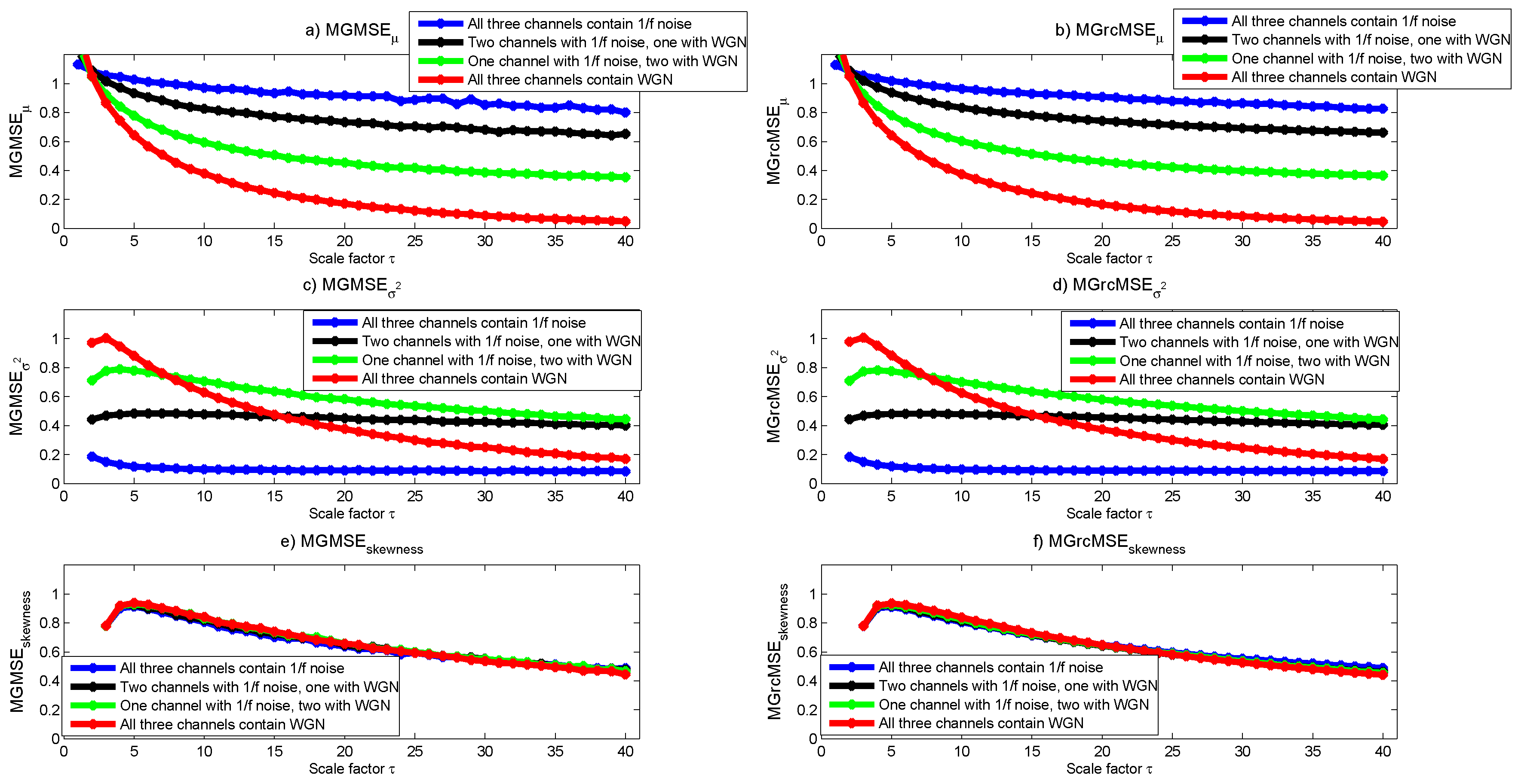
MGMSE and MGrcMSE for similar kinds of data have been previously reported [7,9]: the multivariate sample entropy decreases with increasing scale factors, whatever the composition of the multivariate data (see Figure 2a,b). Moreover, for scale factors larger than 2, the higher the number of variates representing noise, the higher the multivariate entropy value. We observe that the results obtained with MGMSE and MGrcMSE are similar. However, for the largest scales, we observe some wandering on MGMSE that is not visible on MGrcMSE.
The results given by MGMSE and MGrcMSE are shown in Figure 2c,d. We note a slight increase and then a decrease of the multivariate sample entropy with increasing scale factors, except for the trivariate data containing only noise, where a nearly constant multivariate sample entropy is observed for increasing scale factors. For scales lower than 40, the multivariate data with channels containing only white noise show higher multivariate sample entropy than multivariate data with channels containing only noise. Others have reported similar findings for univariate data [19]. Therefore, the scale for which the multivariate data containing only noise shows larger entropy values than those of multivariate data containing only white noise is larger than what was observed with MGMSE: for scales lower than 40, trivariate data containing channels with only noise have a lower multivariate sample entropy than trivariate data containing channels with only white noise; for MGMSE, for scales larger than 2, trivariate data containing channels with only noise have a larger multivariate sample entropy than trivariate data containing channels with only white noise (see Figure 2a,b). If we focus on the decrease rate observed for MGMSE and MGrcMSE, we can say that the results are consistent with what was expected: the more the multivariate data contain noise, the slower the decrease of the multivariate sample entropy values with increasing scale factors ( data are theoretically more complex than white noise, because data contain long-range correlations [2]). Moreover, we observe that the results obtained with MGMSE and MGrcMSE are rather similar.
The results obtained by computing MGMSE and MGrcMSE are shown in Figure 2e,f. We observe that—whatever the composition of the multivariate dataset—the multivariate sample entropy first increases until scale factor , and then decreases. For MGrcMSE, the most rapid decrease is observed for data with channels containing only white noise. The slowest decrease is observed for data with channels containing only noise. For scale factors larger than 20, the highest multivariate sample entropy is observed for data with channels containing only noise, and the lowest for data with channels containing only white noise. The global trend for MGMSE is similar to the one of MGrcMSE, but the different rates of decrease for each variate are not as clear as for MGrcMSE.
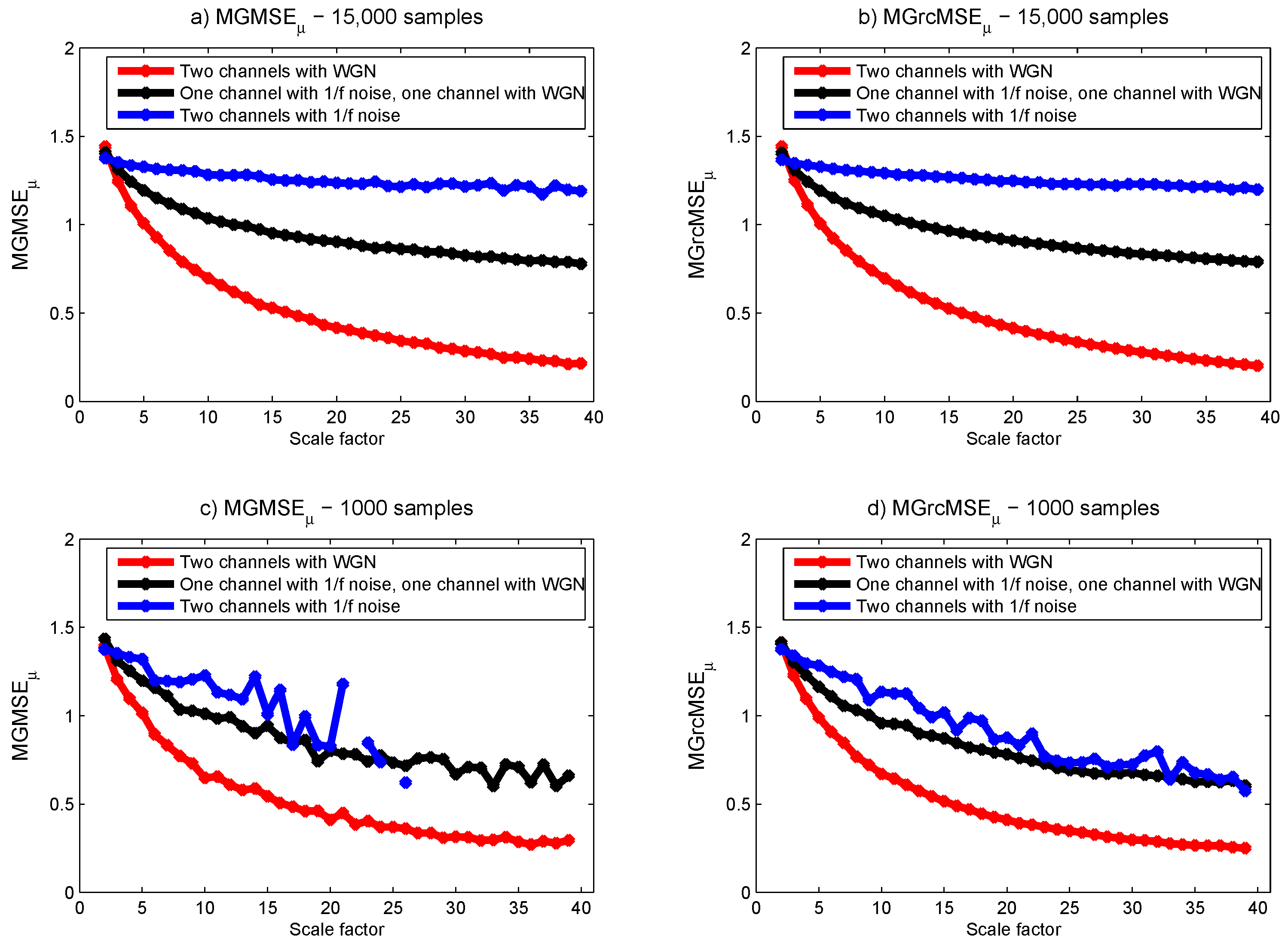
The same analysis was also performed for synthesized bivariate data (as are the biomedical datasets processed thereafter): originally, the two data channels were realizations of mutually independent white noise [7]. We then gradually decreased the number of variates representing white noise (from 2 to 0), and simultaneously increased the number of data channels representing independent noise (from 0 to 2). The shortest experimental bivariate data processed thereafter (EEG data) contain 1000 samples. Therefore, we computed MGMSE and MGrcMSE for two different synthesized bivariate data: one containing 15,000 samples and another containing 1000 samples. Our goal is to analyze if the results obtained for the two lengths (15,000 and 1000 samples) are similar. For this purpose, we considered only scales lower than 10, as data with only 1000 samples do not reasonably allow us to go beyond this limit. Thus, for data with 15,000 samples, the shortest coarse-grained time series has a length of 1500 samples. For data with 1000 samples, the shortest coarse-grained time series has a length of 100 samples. For this last case, the length of the coarse-grained time series will therefore be lower than 300, as recommended by others [8,18]. With a length of 100 samples, the results obtained with MGrcMSE should still be acceptable, as shown in [9]. For each length (15,000 samples and 1000 samples), 10 independent realizations were simulated.
For data with 15,000 samples, MGMSE and MGrcMSE show consistent results with those observed for trivariate datasets (see Figure 3a,b). However, for data with 1000 samples, we observe that MGMSE leads to undefined entropy values (see Figure 3c). MGrcMSE shows similar values to those obtained with 15,000 samples—except for the bivariate data containing only noise, where wandering are observed (see Figure 3d). However, for scales lower than 10, the results obtained with MGrcMSE are still acceptable.
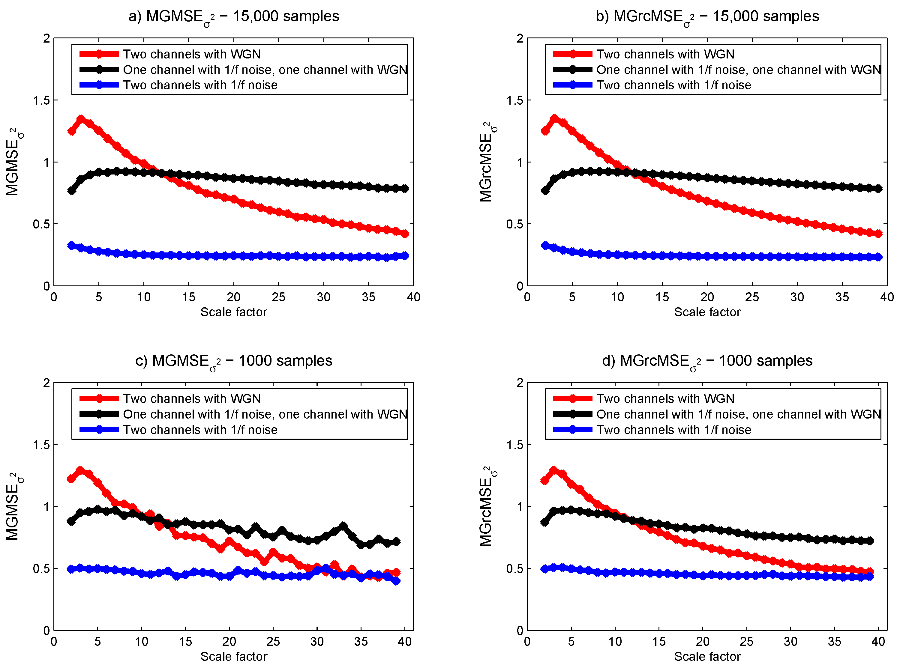
For MGMSE and MGrcMSE (see Figure 4), the bivariate data containing only time series present almost constant multivariate sample entropy values with increasing scale factors. However, for the bivariate data containing only white noise and for the bivariate data containing both noise and white noise, we observe an increase and then a decrease of the multivariate sample entropy for increasing scale factors. We also observe that MGMSE shows different results for data of 15,000 samples and for data of 1000 samples. However, MGrcMSE shows close findings for the two lengths.
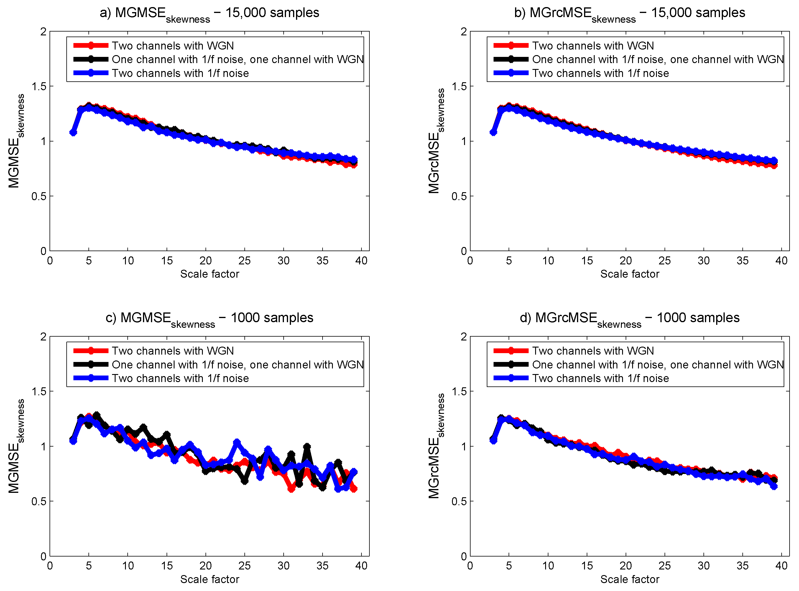
For MGMSE and MGrcMSE, the results show that—whatever the composition of the bivariate dataset—the behavior is the same as scales increase (see Figure 5). We observe an increase of the multivariate sample entropy with increasing scale factors and then a progressive decrease. However, as above, MGrcMSE shows more stable results for short time series than MGMSE where wandering are observed.
From all these results obtained with a bivariate dataset, we observe that the findings obtained with 15,000 samples and with 1000 samples show differences when the data are processed with MGMSE. When MGrcMSE is used, the differences are much less pronounced. For scales lower than 10, MGrcMSE computed with 1000 samples leads to consistent results with those obtained with 15,000 samples. This is true for MGrcMSE, MGrcMSE, and MGrcMSE. In what follows, we will therefore concentrate on the refined versions of the multivariate generalized entropy measures: MGrcMSE, MGrcMSE, and MGrcMSE.
3.2. Results for Biomedical Datasets
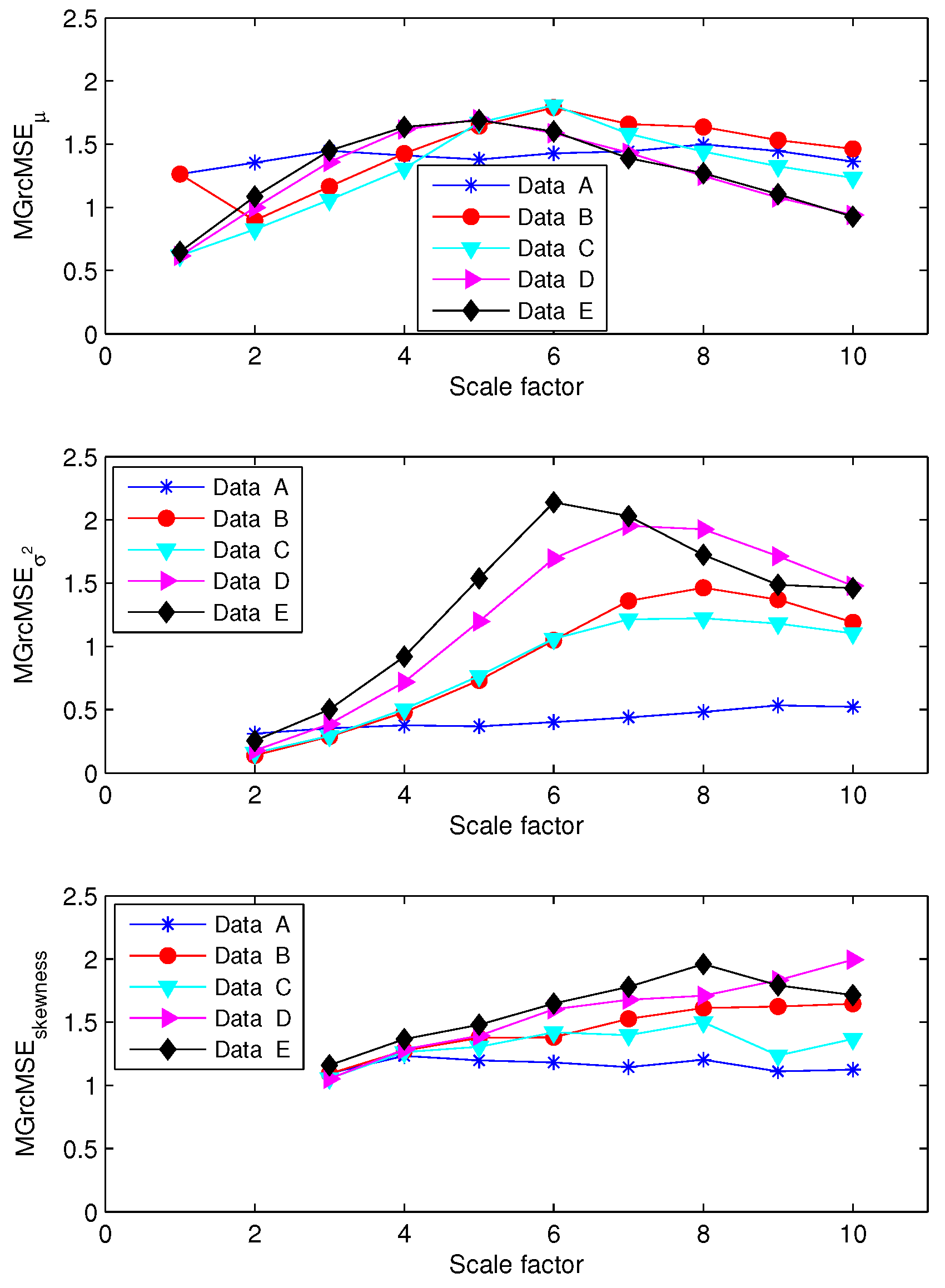
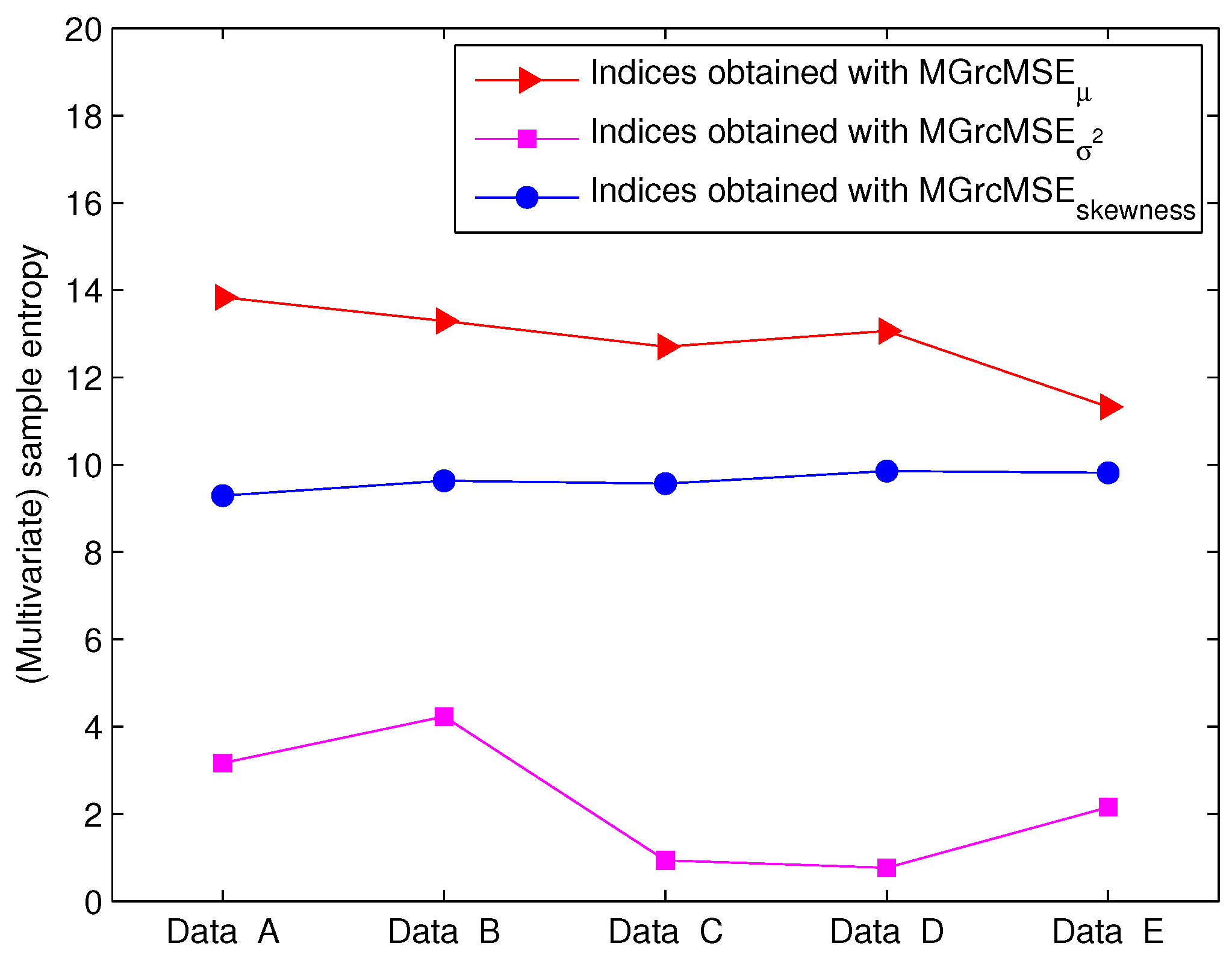
For the first set of EEG data (EEG recorded in rats), the results obtained applying MSE to each channel independently are presented in Figure 6. We note that the sample entropy values for the five pairs of rat EEG signals are close to each other. From this, it seems therefore difficult to distinguish the five cases. The results obtained with MGrcMSE, MGrcMSE, and MGrcMSE are presented in Figure 7. We observe that MGrcMSE, MGrcMSE, and MGrcMSE show different patterns for each of the five cases. However, the highest differences between the five cases are given by MGrcMSE. In order to more easily quantify these differences, we propose the computation of a complexity index, defined here as the sum of the (multivariate) sample entropy for all scales studied. The computation of a similar index has been performed in other studies (e.g., [20,21,22,23]). For the univariate case, the sum was computed for each channel independently, and then the mean of the two sums was considered. The results for each case are presented in Figure 8. We observe that MGrcMSE leads to a better distinction of the different cases than MGrcMSE. Data B, C, D, and E all contain spike-wave discharges. Therefore, we could have expected to obtain similar signatures for MGrcMSE and/or for MGrcMSE. However, we obtain different results on these datasets. This is consistent with other synchronization measures which were also able to distinguish them [15]. Contents of data B, C, D, and E are therefore different. Our findings suggest that the multivariate multiscale complexity of the volatility may be more interesting than MGrcMSE when studying multivariate datasets.
For the second set of EEG data (EEG recorded in humans), the results obtained applying MSE to each channel independently are presented in Figure 9. We note that the sample entropy of the five cases are close to each other. Therefore, their differentiation is hardly possible. The results obtained with MGrcMSE, MGrcMSE, and MGrcMSE are presented in Figure 10. We observe that MGrcMSE, MGrcMSE, and MGrcMSE facilitate the differentiation between the five cases. However, the highest differences between the five cases are given by MGrcMSE. As above (and with the same definition as above), we computed the complexity index. The results for each case are presented in Figure 11. As previously, we observe that MGrcMSE leads to a better distinction of the five cases than MGrcMSE.
As mentioned above, the coarse-graining procedure can be seen as a FIR (low-pass filter) on the original time series and to the downsampling of the filtered signal with a factor τ [11]. This multiscale procedure is reminiscent of multiscale transforms such as wavelet, ridgelet, or curvelet transforms [24,25,26,27]. Such transforms can also be used with entropy measures.
Our work is still in progress. The analysis performed on the synthetic data has to be continued, and many more real datasets have to be analyzed in order to obtain a better understanding of the potentialities of MGMSE and MGrcMSE. However, the first findings presented herein are encouraging. Nevertheless, our study presents limitations. A first limitation is the non-existence of an inverse transform for this multiscale transform. Another limitation is the computational time of MGMSE (and even more, the one of MGrcMSE): this computational time prevents real-time analyses. This is particularly annoying, as we need to record long time series if large scales are to be analyzed.
Therefore, for the future, several directions could be studied. To improve the time complexity of MSE, several algorithms have been proposed [28,29,30,31]. It could now be interesting to adapt these algorithms to the multivariate case, and to study MGMSE and MGrcMSE based on these faster codes. Furthermore, the original MSE relies on a sample entropy-based approach, but can be used with different types of entropic measures: permutation entropy, cross-approximate entropy, compression entropy, etc. The multivariate generalization proposed herein could be extended to MSE based on other entropic measures. In addition to rcMSE, several other variants to MSE have been proposed: refined MSE [11], composite MSE [12], modified MSE for short-term time series [10], and short time MSE [32], to cite only a few. The multivariate approach of these variants could now be proposed, as well as their generalization to higher moments. For our simulated time series, MGrcMSE leads to close values, whatever the composition of the multivariate dataset. These results have to be studied more thoroughly in the future. However, we observe that different findings are obtained for EEG data. For the univariate case, MSE has already been shown to give interesting results for the biomedical field [33].
4. Conclusions
MSE is now widely used in a large number of areas. Its refined version (rcMSE) has also been proposed to improve the results when processing short time series. Their adaptation to multivariate data exist (MMSE and MrcMSE). MSE, rcMSE, MMSE, and MrcMSE rely (among others) on a coarse-graining procedure to obtain a set of time series representing the system dynamics on different time scales. In this coarse-graining procedure, the computation of the mean (first moment) of samples inside consecutive windows is performed. A generalization of MSE has recently been proposed. This generalization consists of using other moments in the coarse-graining procedure. Unfortunately, this generalization did not exist for multivariate datasets. We therefore herein proposed an extension of this generalized MSE to multivariate datasets. We first analyzed the behavior of MGMSE and MGrcMSE on synthetic signals, and processed two different publicly available bivariate EEG data sets. Our results show that MGrcMSE may present better performance than MrcMSE in differentiating different types of EEG signals. MGrcMSE could therefore become an interesting signal processing tool for multivariate datasets. Moreover, we have shown that MGMSE and MGrcMSE lead to similar results when long data are analyzed. However, MGrcMSE shows better performance than MGMSE when short data are processed. The time complexity of MGrcMSE being worse than the one of MGMSE, we suggest the use of MGMSE for long data and MGrcMSE for short data.
In our work, the parameter r was kept constant, as done in other studies [6,19]. However, the coarse-graining procedure is similar to smoothing and decimation of the original sequences [34]. Because the same parameter r is used for all scales, in MSE, some authors concluded that the changes in MSE on each scale depend on both the regularity and variation of the coarse-grained time series [34]. More work could therefore be conducted to analyze the results when adapting the parameter r to each scale or for each moment used [33].
Our new method has been applied to EEG data. After a deeper analysis of synthetic time series, multivariate magnetoencephalography data could also be analyzed, but also data recorded simultaneously by different modalities. This could help in the diagnosis of pathologies that affect several organs or systems. For example, the simultaneous acquisition of data from the peripheral and central cardiovascular systems and their analysis with MG(rc)MSE could help in the understanding and diagnosis of some cardiovascular diseases. MG(rc)MSE could also be used for many other kinds of data: financial time series, chemical data, etc.
Acknowledgments
Anne Humeau-Heurtier would like to acknowledge Thomas Kreuz for fruitful discussions.
Conflicts of Interest
The author declares no conflict of interest.
References
- Costa, M.; Goldberger, A.L.; Peng, C.K. Multiscale entropy analysis of complex physiologic time series. Phys. Rev. Lett. 2002, 89, 068102. [Google Scholar] [CrossRef] [PubMed]
- Costa, M.; Goldberger, A.L.; Peng, C.K. Multiscale entropy analysis of biological signals. Phys. Rev. E 2005, 71, 021906. [Google Scholar] [CrossRef] [PubMed]
- Richman, J.S.; Moorman, J.R. Physiological time-series analysis using approximate entropy and sample entropy. Am. J. Physiol. Heart Circ. Physiol. 2000, 278, H2039–H2049. [Google Scholar] [PubMed]
- Humeau-Heurtier, A. The multiscale entropy algorithm and its variants: A review. Entropy 2015, 17, 3110–3123. [Google Scholar] [CrossRef] [Green Version]
- Wu, S.D.; Wu, C.W.; Lin, S.G.; Lee, K.Y.; Peng, C.K. Analysis of complex time series using refined composite multiscale entropy. Phys. Lett. A 2014, 378, 1369–1374. [Google Scholar] [CrossRef]
- Costa, M.D.; Goldberger, A.L. Generalized multiscale entropy analysis: Application to quantifying the complex volatility of human heartbeat time series. Entropy 2015, 17, 1197–1203. [Google Scholar] [CrossRef] [PubMed]
- Ahmed, M.U.; Mandic, D.P. Multivariate multiscale entropy: A tool for complexity analysis of multichannel data. Phys. Rev. E 2011, 84, 061918. [Google Scholar] [CrossRef] [PubMed]
- Ahmed, M.U.; Mandic, D.P. Multivariate multiscale entropy analysis. IEEE Signal Process. Lett. 2012, 19, 91–94. [Google Scholar] [CrossRef]
- Humeau-Heurtier, A. Multivariate refined composite multiscale entropy analysis. Phys. Lett. A 2016, 380, 1426–1431. [Google Scholar] [CrossRef] [Green Version]
- Wu, S.D.; Wu, C.W.; Lee, K.Y.; Lin, S.G. Modified multiscale entropy for short-term time series analysis. Physica A 2013, 392, 5865–5873. [Google Scholar] [CrossRef]
- Valencia, J.F.; Porta, A.; Vallverdu, M.; Claria, F.; Baranowski, R.; Orlowska-Baranowska, E.; Caminal, P. Refined multiscale entropy: Application to 24-h Holter recordings of heart period variability in healthy and aortic stenosis subjects. IEEE Trans. Biomed. Eng. 2009, 56, 2202–2213. [Google Scholar] [CrossRef] [PubMed]
- Wu, S.D.; Wu, C.W.; Lin, S.G.; Wang, C.C.; Lee, K.Y. Time series analysis using composite multiscale entropy. Entropy 2013, 15, 1069–1084. [Google Scholar] [CrossRef]
- Available online: http://www2.le.ac.uk/departments/engineering/research/bioengineering/neuroengineering-lab/software (accessed on 5 June 2016).
- Available online: http://epileptologie-bonn.de/cms/frontcontent.php?idcat=193&lang=3 (accessed on 22 October 2016).
- Quian Quiroga, R.; Kraskov, A.; Kreuz, T.; Grassberger, P. Performance of different synchronization measures in real data: A case study on electroencephalographic signals. Phys. Rev. E 2002, 65, 041903. [Google Scholar] [CrossRef] [PubMed]
- Quian Quiroga, R.; Kreuz, T.; Grassberger, P. Event synchronization: A simple and fast method to measure synchronicity and time delay patterns. Phys. Rev. E 2002, 66, 41904. [Google Scholar] [CrossRef] [PubMed]
- Andrzejak, R.G.; Lehnertz, K.; Rieke, C.; Mormann, F.; David, P.; Elger, C.E. Indications of nonlinear deterministic and finite dimensional structures in time series of brain electrical activity: Dependence on recording region and brain state. Phys. Rev. E 2001, 64, 061907. [Google Scholar] [CrossRef] [PubMed]
- Ahmed, M.U.; Rehman, N.; Looney, D.; Rutkowski, T.M.; Mandic, D.P. Dynamical complexity of human responses: A multivariate data-adaptive framework. Bull. Pol. Acad. Sci. Tech. Sci. 2012, 60, 433–445. [Google Scholar] [CrossRef]
- Azami, H.; Fernandez, A.; Escudero, J. Refined Multiscale Fuzzy Entropy Based on Standard Deviation for Biomedical Signal Analysis. 2016; arXiv:1602.02847. [Google Scholar]
- Schnettler, W.T.; Goldberger, A.L.; Ralston, S.J.; Costa, M. Complexity analysis of fetal heart rate preceding intrauterine demise. Eur. J. Obstet. Gynecol. Reprod. Biol. 2016, 203, 286–290. [Google Scholar] [CrossRef] [PubMed]
- Costa, M.; Ghiran, I.; Peng, C.-K.; Nicholson-Weller, A.; Goldberger, A.L. Complex dynamics of human red blood cell flickering: Alterations with in vivo aging. Phys. Rev. E Stat. Nonlinear Soft Matter Phys. 2008, 78, 020901. [Google Scholar] [CrossRef] [PubMed]
- Costa, M.D.; Henriques, T.; Munshi, M.N.; Segal, A.R.; Goldberger, A.L. Dynamical glucometry: Use of multiscale entropy analysis in diabetes. Chaos 2014, 24, 033139. [Google Scholar] [CrossRef] [PubMed]
- Costa, M.D.; Schnettler, W.T.; Amorim-Costa, C.; Bernardes, J.; Costa, A.; Goldberger, A.L.; Ayres-de-Campos, D. Complexity-loss in fetal heart rate dynamics during labor as a potential biomarker of acidemia. Early Hum. Dev. 2014, 90, 67–71. [Google Scholar] [CrossRef] [PubMed]
- Starck, J.-L.; Murtagh, F.; Fadili, J.M. Sparse Image and Signal Processing: Wavelets and Related Geometric Multiscale Analysis, 2nd ed.; Cambridge University Press: Cambridge, UK, 2015; pp. 1–423. [Google Scholar]
- Shuman, D.I.; Faraji, M.J.; Vandergheynst, P. A multiscale pyramid transform for graph signals. IEEE Trans. Signal Process. 2016, 64, 2119–2134. [Google Scholar] [CrossRef]
- Xiao, M.; He, Z. Remote sensing image fusion based on gaussian mixture model and multiresolution analysis. Proc. SPIE 2013, 8921. [Google Scholar] [CrossRef]
- Grohs, P. Geometric multiscale decompositions of dynamic low-rank matrices. Comput. Aided Geom. Des. 2013, 30, 805–826. [Google Scholar] [CrossRef]
- Sugisaki, K.; Ohmori, H. Online estimation of complexity using variable forgetting factor. In Proceedings of the 2007 SICE Annual Conference, Takamatsu, Japan, 17–20 September 2007; pp. 1–6.
- Samani, A.; Madeleine, P. Permuted sample entropy. Commun. Stat. Simul. Comput. 2010, 39, 1506–1516. [Google Scholar] [CrossRef]
- Pan, Y.H.; Lin, W.Y.; Wang, Y.H.; Lee, K.T. Computing multiscale entropy with orthogonal range search. J. Mar. Sci. Technol. 2011, 19, 107–113. [Google Scholar]
- Jiang, Y.; Mao, D.; Xu, Y. A fast algorithm for computing sample entropy. Adv. Adapt. Data Anal. 2011, 3, 167–186. [Google Scholar] [CrossRef]
- Chang, Y.C.; Wu, H.T.; Chen, H.R.; Liu, A.B.; Yeh, J.J.; Lo, M.T.; Tsao, J.H.; Tang, C.J.; Tsai, I.T.; Sun, C.K. Application of a modified entropy computational method in assessing the complexity of pulse wave velocity signals in healthy and diabetic subjects. Entropy 2014, 16, 4032–4043. [Google Scholar] [CrossRef]
- Shi, W.; Shang, P.; Ma, Y.; Sun, S.; Yeh, C.H. A comparison study on stages of sleep: Quantifying multiscale complexity using higher moments on coarse-graining. Commun. Nonlinear Sci. Numer. Simul. 2017, 44, 292–303. [Google Scholar] [CrossRef]
- Nikulin, V.V.; Brismar, T. Comment on “Multiscale entropy analysis of complex physiologic time series”. Phys. Rev. Lett. 2004, 92, 089803. [Google Scholar] [CrossRef] [PubMed]
Figure 1.
Flow chart describing the computation of multivariate extension of generalized refined composite multiscale entropy (MGrcMSE) for a p-variate time series ( is the channel index, and N is the number of samples in every channel).
Figure 1.
Flow chart describing the computation of multivariate extension of generalized refined composite multiscale entropy (MGrcMSE) for a p-variate time series ( is the channel index, and N is the number of samples in every channel).
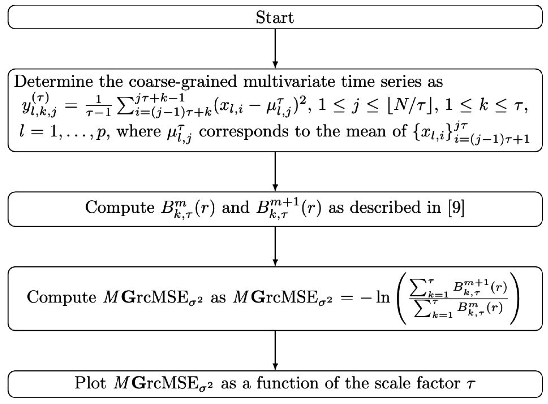
Figure 2.
(a) multivariate extension of the generalized MSE (MGMSE); (b) MGrcMSE; (c) MGMSE; (d) MGrcMSE; (e) MGMSE; and (f) MGrcMSE average values for ten trivariate data containing white Gaussian noise (WGN) and noise, each with 15,000 samples.
Figure 2.
(a) multivariate extension of the generalized MSE (MGMSE); (b) MGrcMSE; (c) MGMSE; (d) MGrcMSE; (e) MGMSE; and (f) MGrcMSE average values for ten trivariate data containing white Gaussian noise (WGN) and noise, each with 15,000 samples.

Figure 3.
MGMSE (left column) and MGrcMSE (right column) average values for ten bivariate data containing white Gaussian noise (WGN) and noise, each with 15,000 samples (upper panels) and 1000 samples (lower panels).
Figure 3.
MGMSE (left column) and MGrcMSE (right column) average values for ten bivariate data containing white Gaussian noise (WGN) and noise, each with 15,000 samples (upper panels) and 1000 samples (lower panels).

Figure 4.
MGMSE (left column) and MGrcMSE (right column) average values for ten bivariate data containing white Gaussian noise (WGN) and noise, each with 15,000 samples (upper panels) and 1000 samples (lower panels).
Figure 4.
MGMSE (left column) and MGrcMSE (right column) average values for ten bivariate data containing white Gaussian noise (WGN) and noise, each with 15,000 samples (upper panels) and 1000 samples (lower panels).

Figure 5.
MGMSE (left column) and MGrcMSE (right column) average values for ten bivariate data containing white Gaussian noise (WGN) and noise, each with 15,000 samples (upper panels) and 1000 samples (lower panels).
Figure 5.
MGMSE (left column) and MGrcMSE (right column) average values for ten bivariate data containing white Gaussian noise (WGN) and noise, each with 15,000 samples (upper panels) and 1000 samples (lower panels).

Figure 6.
MSE values for five electroencephalogram (EEG) cases (data A to E, from top to bottom). For each subplot, each curve corresponds to a data channel. Data A correspond to a normal EEG, and data B, C, D, and E contain spike-wave discharges [15,16].
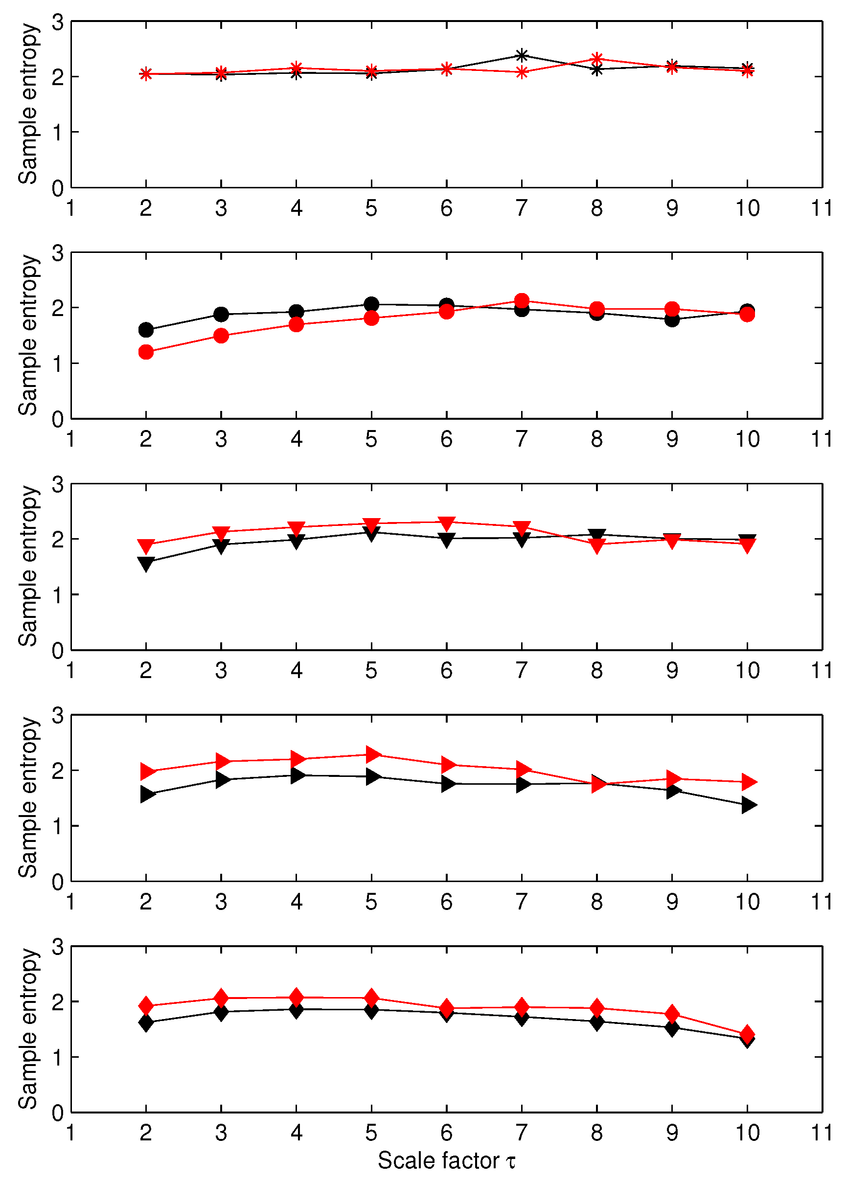
Figure 7.
From top to bottom: MGrcMSE, MGrcMSE, and MGrcMSE for five pairs of rat EEG signals—see Figure 6.
Figure 7.
From top to bottom: MGrcMSE, MGrcMSE, and MGrcMSE for five pairs of rat EEG signals—see Figure 6.

Figure 8.
Complexity index for five EEG cases—see Figure 6.
Figure 8.
Complexity index for five EEG cases—see Figure 6.
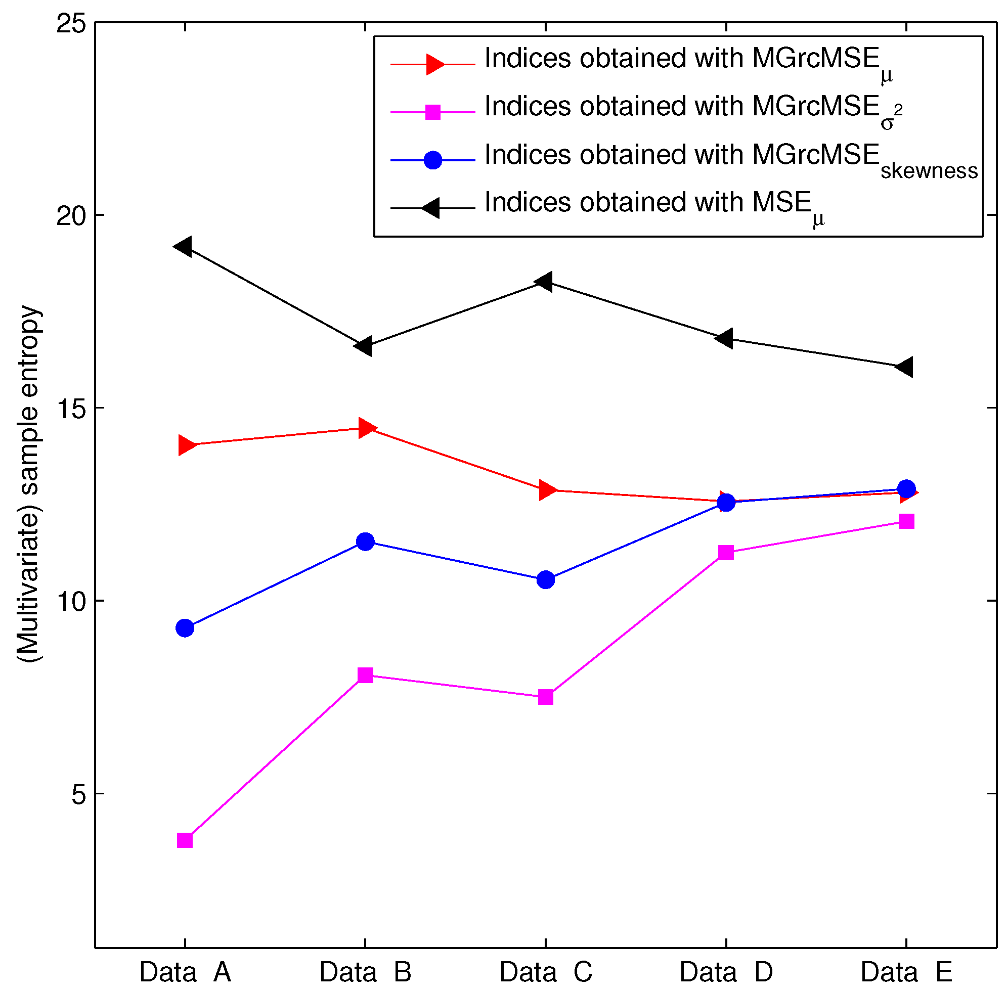
Figure 9.
MSE values for five EEG cases (data A to E, from top to bottom). For each subplot, each curve corresponds to a data channel. See text for details on each data set, and [17] for the data acquisition procedure.
Figure 9.
MSE values for five EEG cases (data A to E, from top to bottom). For each subplot, each curve corresponds to a data channel. See text for details on each data set, and [17] for the data acquisition procedure.
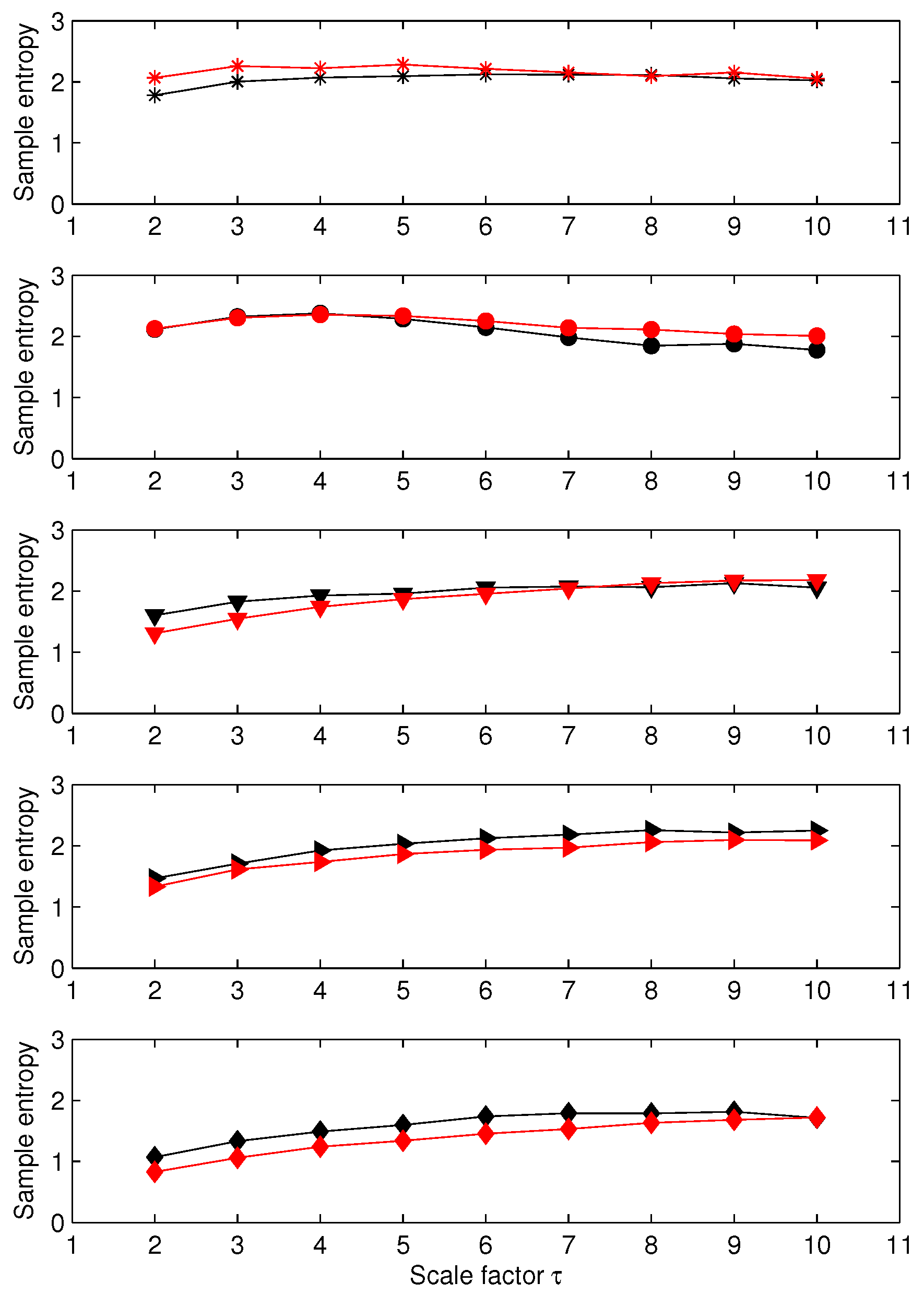
Figure 10.
From top to bottom: MGrcMSE, MGrcMSE, and MGrcMSE for five pairs of human EEG signals—see Figure 9.
Figure 10.
From top to bottom: MGrcMSE, MGrcMSE, and MGrcMSE for five pairs of human EEG signals—see Figure 9.
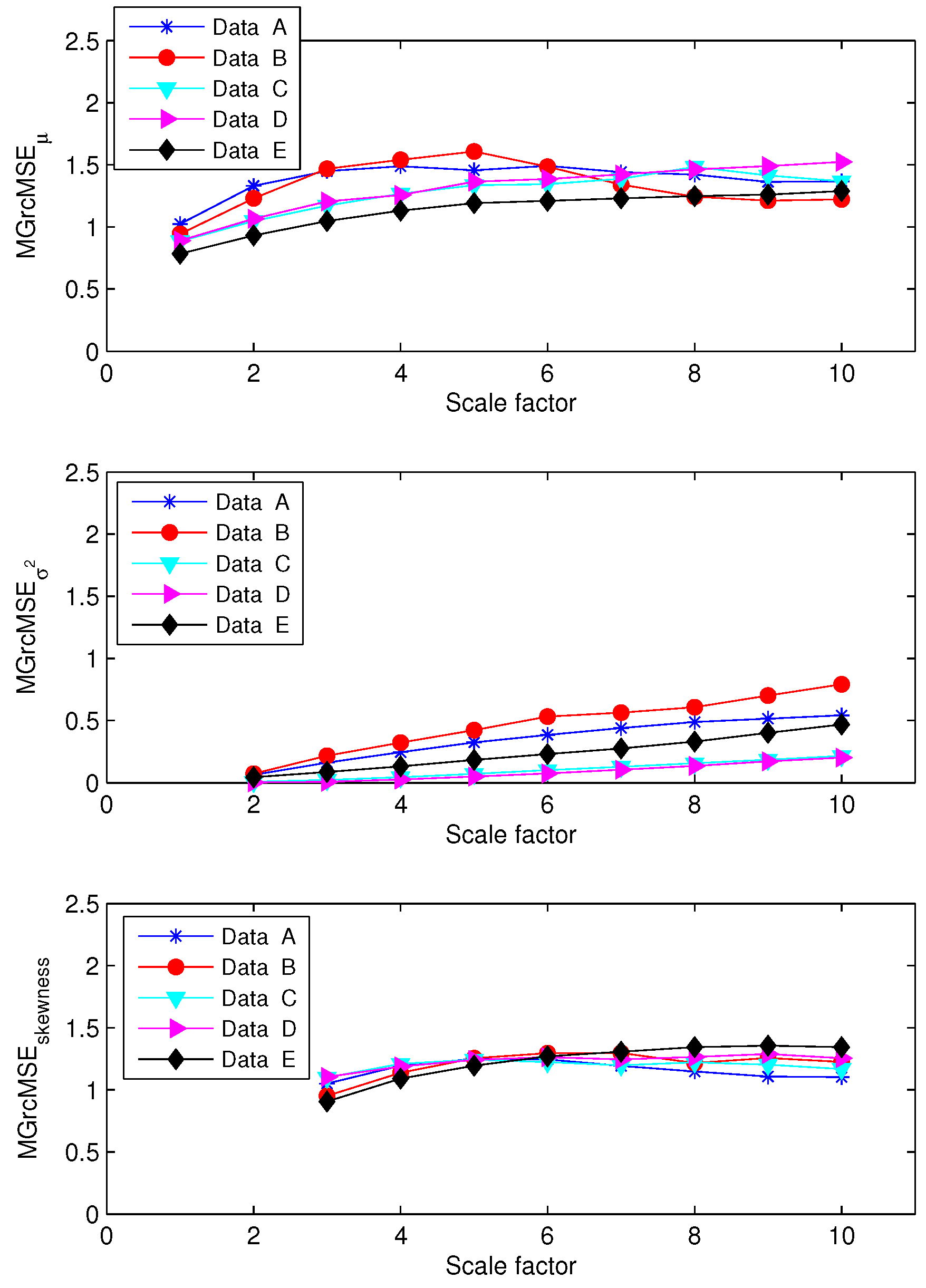
Figure 11.
Complexity index for five EEG cases—see Figure 9.
Figure 11.
Complexity index for five EEG cases—see Figure 9.

© 2016 by the author; licensee MDPI, Basel, Switzerland. This article is an open access article distributed under the terms and conditions of the Creative Commons Attribution (CC-BY) license (http://creativecommons.org/licenses/by/4.0/).
Share and Cite
MDPI and ACS Style
Humeau-Heurtier, A. Multivariate Generalized Multiscale Entropy Analysis. Entropy 2016, 18, 411. https://doi.org/10.3390/e18110411
AMA Style
Humeau-Heurtier A. Multivariate Generalized Multiscale Entropy Analysis. Entropy. 2016; 18(11):411. https://doi.org/10.3390/e18110411
Chicago/Turabian StyleHumeau-Heurtier, Anne. 2016. "Multivariate Generalized Multiscale Entropy Analysis" Entropy 18, no. 11: 411. https://doi.org/10.3390/e18110411
Note that from the first issue of 2016, this journal uses article numbers instead of page numbers. See further details here.