Texture Segmentation Using Laplace Distribution-Based Wavelet-Domain Hidden Markov Tree Models

Abstract

Multiresolution models such as the wavelet-domain hidden Markov tree (HMT) model provide a powerful approach for image modeling and processing because it captures the key features of the wavelet coefficients of real-world data. It is observed that the Laplace distribution is peakier in the center and has heavier tails compared with the Gaussian distribution. Thus we propose a new HMT model based on the two-state, zero-mean Laplace mixture model (LMM), the LMM-HMT, which provides significantly potential for characterizing real-world textures. By using the HMT segmentation framework, we develop LMM-HMT based segmentation methods for image textures and dynamic textures. The experimental results demonstrate the effectiveness of the introduced model and segmentation methods.

1. Introduction

Texture is an important component of natural images, which provides abundant cues for visual information recognition and understanding. It’s generally recognized that the image texture is defined as a function of the spatial variation in pixel gray values, which is useful in a variety of applications, such as medical image analysis, document processing and remotely sensed image analysis [1]. Recently, dynamic texture analysis has attracted much attention. Dynamic textures are video sequences of complex dynamical objects such as smoke, fire, sea waves, foliage waving in wind, moving escalators, and swinging flags, which exhibit certain stationary properties in time [2]. They provide important visual cues for various video processing problems. Therefore, texture analysis is still an important and interesting research field [3,4,5,6,7,8].

Image (video) segmentation attempts to partition an image (video) into regions, each of which has a reasonably homogeneous visual appearance or corresponds to an object or a part of the object [9]. Multiscale Bayesian approaches for texture segmentation have been proven efficient to integrate both features and the contextual information into the estimation of class labels. In [10,11], a tree-structured hidden Markov model, hidden Markov tree (HMT) model, was proposed in the wavelet-domain to achieve the statistical characterization of signals and images by capturing interscale dependencies of wavelet coefficients across scales. The multiscale dependencies tying together the hidden states assigned to the coefficients rather than their values, is the fundamental difference with other multiscale Markovian model. In [12], Durand presented an alternative upward-downward algorithm for smoothed probabilities, which is a true smoothing algorithm that is immune to underflow problems in the HMT model and whose complexity remains unchanged. The segmentation method derived in [13], HMTseg, has been proved as a very useful solution by combining the parametric wavelet-domain statistical modeling, direct likelihood calculation, and multiscale Bayesian decision fusion. In [14], Ye proposed a novel texture descriptor for vision-based smoke detection using a Surfacelet transform and 3D HMT model, proving that the HMT model can be used to obtain high detection accuracy, and has a wide range of applications, such as object recognition. In [15], Wang took advantage of the pyramidal dual-tree directional filter bank (PDTDFB) transform, and proposed a new color image segmentation algorithm based on PDTDFB domain HMT model.

In order to match the compression property of the wavelet transform that the majority of coefficients have small values and the minority of coefficients have large values, the marginal distribution $f_W\left(w_i\right)$ of each coefficient node $w_i$ of the traditional HMT model is modeled as Gaussian mixture model (GMM) that is a mixture of Gaussian conditional distributions. In many applications, for example texture analysis and image restoration [16], the GMM has been proved to be effective. However, for the histograms of some image textures and dynamic textures, such as “Floor” shown in Figure 1, the Laplace mixture model (LMM) provides a better fitness to the histogram than the Gaussian mixture model, because the histogram is peakier in the center and has heavier tails. That is to say, LMM can describe the marginal distribution of $f_W\left(w_i\right)$ better. The results on texture classification [17] and image denoising [18,19] also demonstrate the potential of Laplace distributions and their mixtures for the prior image. Therefore, we introduce Laplace mixture distribution-based HMT models to model the wavelet coefficient distributions of textures.

The rest of this paper is organized as follows: in Section 2, we briefly review the basic concepts of the Laplacian distribution, HMT models, and the multiscale image segmentation method based on HMT models. In Section 3, we propose the LMM-based HMT model and its parameter estimation. For more accurate texture characterization, we also use Laplace mixture distribution to describe the pixel-level texture. In Section 4, we introduce LMM-HMT-based image texture segmentation and dynamic texture segmentation. Experimental results are shown and analyzed in the fifth section, and then the conclusions are given in the last section.

2. Previous Works

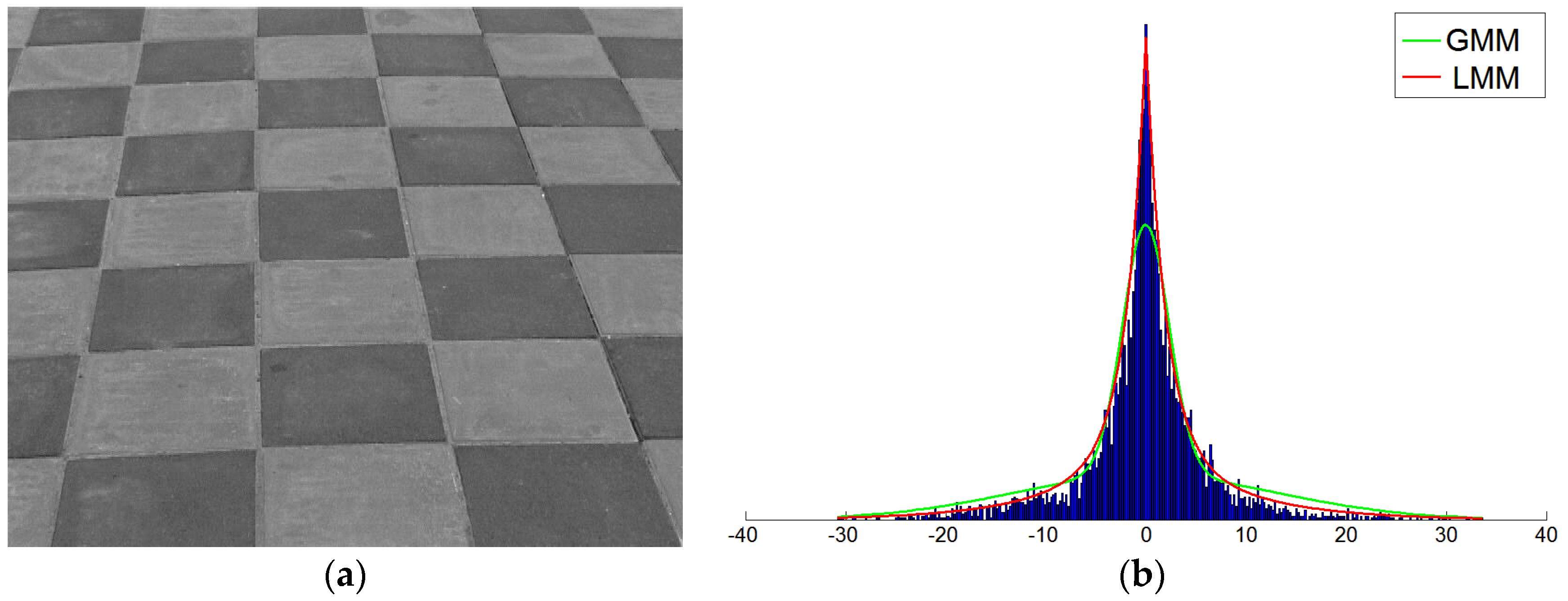
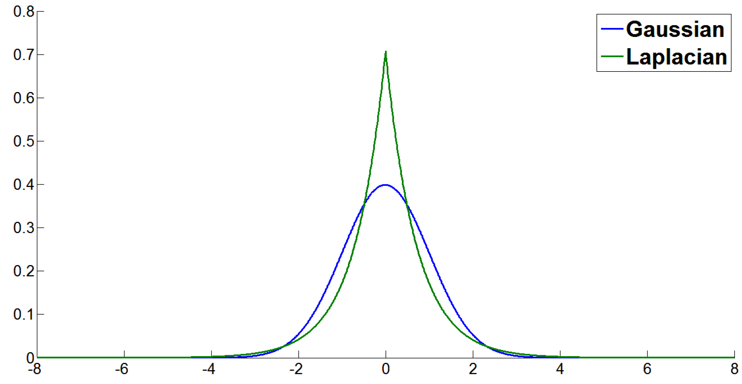
2.1. Laplacian Distribution

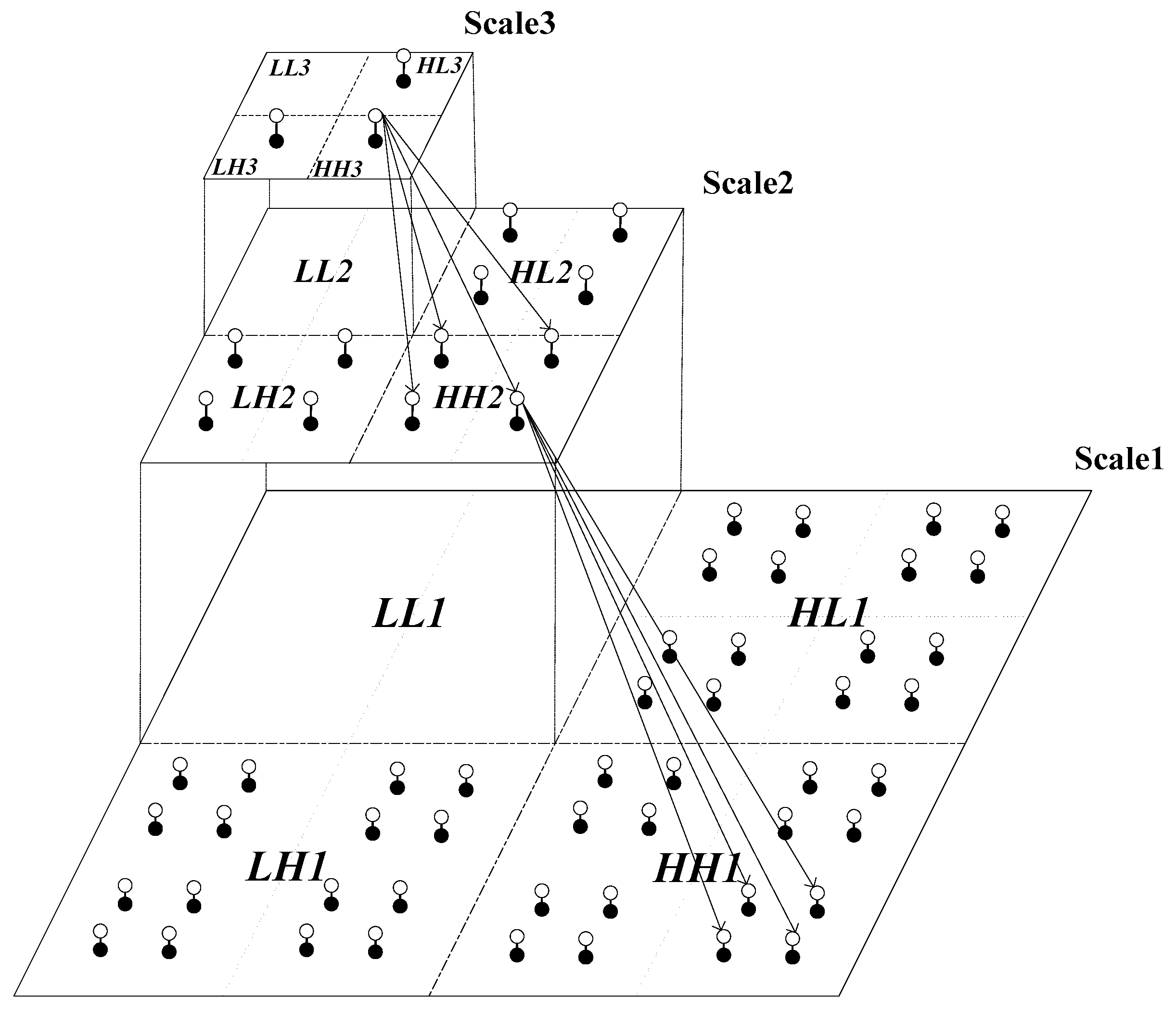
The classical Laplacian distribution is symmetrical and leptokurtic (peaky), which is also referred to as the double exponential distribution and widely applied in many fields [20]. For example, it can be used to model the difference between the waiting times of two events generated by two random processes, describe breaking strength data, and model the differences in flood stages, etc. A Laplacian distribution has a probability density function (pdf):

$$l\left(x;a,b\right)=\frac{1}{2b}\text{exp}\left[-\frac{\left|x-a\right|}{b}\right]=\frac{1}{2b}\{\begin{array}{c}\text{exp}\left(-\frac{a-x}{b}\right) x<a\\ \text{exp}\left(-\frac{x-a}{b}\right) x\ge a\end{array}$$

(1)

where a is the location parameter and b is the scale parameter. As shown in Figure 2, since a Laplacian distribution is represented by the absolute difference of all samples from their mean, while a Gaussian distribution is represented by the squared difference of all samples from their mean, the Laplacian distribution can be used for modeling data that have heavier tails than those of the Gaussian distribution.

2.2. HMT Models

For real images, the wavelet transform (decomposition) can be used to obtain the multiscale representation, which includes a scaling coefficient sub-band (LL) and three wavelet coefficient sub-bands, the horizontal sub-band (LH), vertical sub-band (HL), and diagonal sub-band (HH), at each level (scale). The histograms of the discrete wavelet transform (DWT) coefficients reveal sparsity, which means that the shape of the marginal probability distribution for wavelet coefficients is peaky in the center and heavy tailed with relatively few large coefficients corresponding to singularities and many small ones from smooth regions. Hence, we consider the collection of large coefficients as outcomes of a pdf with a large variance, and small coefficients as outcomes of a pdf with a small variance. In the wavelet-domain HMT model, this non-Gaussian nature is matched as a Gaussian mixture density with a hidden state that dictates whether a coefficient is large or small. Generally, the Gaussian mixture distribution model of the wavelet coefficient $w_i$ with $M$ components is given as follows:

$$f\left(w_i\right)={\displaystyle \sum _{m=1}^M}{p}_{S_i}\left(m\right)f\left(w_i| S_i=m\right)$$

(2)

where $p_{S_i}\left(m\right)$ is the probability of the m-th hidden state (component), which represents the mixing coefficient or weight, ${\sum }_{m=1}^M{p}_{S_i}(m)=1$. The function $f(w_i|S_i=m)~N({\mu }_{i,m},{\sigma }_{i,m}^2)$ is a Gaussian density with mean ${\mu }_{i,m}$ and variance ${\sigma }_{i,m}^2$. In the wavelet domain HMT model, $M$ is always set to be 2 [10,13].

To capture the mutual dependencies between wavelet coefficients across scales, the HMT uses a probabilistic tree to model Markovian dependencies between the hidden states. Those dependencies tie together the hidden states assigned to the coefficients rather than their values. The values of the wavelet coefficients are the realizations of the Gaussian mixture density $f\left(w_i\right)$. In general, these random variables are treated as independent given the hidden states due to the parameter estimation of HMT. In the pyramid quad-tree structure of the wavelet transform, four children wavelet coefficients divide the spatial localization of the parent coefficients. As shown as Figure 3, each white node denotes the hidden state variable S, and the black node represents a wavelet coefficient W that is a random variable, from which the HMT model is constructed.

An HMT model is specified in terms of the probability of a state at the root node in the coarsest scale, the state transition probabilities and the parameters of the pdf given the state. As shown in Figure 3, a complete image wavelet decomposition comprises three parallel quad-tree structures. With the sub-band independence assumption, a 2D image wavelet domain HMT model consists of three HMT’s [13]. For example, the HH directional sub-bands is characterized by a HMT model with the parameter set ${\mathrm{\Theta }}^{HH}=\left\{p_{\mathrm{J}}\left(m\right),{\mathsf{\epsilon }}_{i,\rho \left(i\right)}^{m,n},{\mu }_{i,m},{\sigma }_{i,m}^2|m,n=0,1;i=1,\cdots ,P\right\}$, in which $p_{\mathrm{J}}\left(m\right)$ is the probablility of a state at the coarsest scale J, ${\mathsf{\epsilon }}_{i,\rho \left(i\right)}^{m,n}$ is the state transition probability ($i>1$), m and n are used to denote the states, $\rho \left(i\right)$ is the parent node of i, P is the total number of the wavelet coefficient of the quad-tree, ${\mu }_{i,m}$ and ${\sigma }_{i,m}^2$ are the parameters of the Guassian distribution. Thus the HMT model of a texture is parameterized by a parameter set $ℳ=\left\{{\mathrm{\Theta }}^{LH},{\mathrm{\Theta }}^{HL},{\mathrm{\Theta }}^{HH}\right\}$, where ${\mathrm{\Theta }}^{LH},{\mathrm{\Theta }}^{HL}$ and ${\mathrm{\Theta }}^{HH}$ are parameters of LH, HL and HH directional sub-bands, respectively, which can be estimated with the tree-structure Expectation-Maximization (EM) algorithm [10,13,21].

2.3. EM Algorithm

It is assumed that there is a data set $\mathcal{X}=\left\{x_1,\cdots ,x_N\right\}$ and these vectors are independent and identically distributed with the distribution p. Then we can construct the (log) likelihood function and estimate the unknown parameters $\mathrm{\Theta }$ with the maximum likelihood method. However, it may impossible to find the analytical solution for many problems, for example, the parameter estimation of a mixture of distributions. The EM algorithm [22] is an alternative method of finding the maximum likelihood estimation of the parameters.

It is well known that the EM algorithm is for computing the maximum likelihood estimates from the incomplete data. The data set $\mathcal{X}$ is the observed samples. We call $\mathcal{X}$ the incomplete data. We assume that $\mathcal{Z}=\left(\mathcal{X},\mathcal{Y}\right)$ is a complete data set. Our goal is to maximize the incomplete log-likelihood function $ln\left(p\left(\mathcal{X}|\mathrm{\Theta }\right)\right)$. The EM algorithm decomposes this difficult maximization into an iteration between two simpler steps: the E step and the M step.

• E step: Computes the conditional expectation of the complete log-likelihood, given the observed data $\mathcal{X}$ and the current estimate ${\widehat{\mathrm{\Theta }}}^t$ as follows:

  $$\mathrm{Q}(\mathrm{\Theta }|{\widehat{\mathrm{\Theta }}}^t)=\mathrm{E}[ln(p(\mathcal{X},\mathcal{Y}|\mathrm{\Theta }))|\mathcal{X},{\widehat{\mathrm{\Theta }}}^t]$$

  (3)
• M step: Update the parameters by maximizing the function:

  $${\widehat{\mathrm{\Theta }}}^{t+1}=\underset{\mathrm{\Theta }}{\text{argmax}} \mathrm{Q}(\mathrm{\Theta }|{\widehat{\mathrm{\Theta }}}^t)$$

  (4)

These two steps are iterated as necessary. It is well known that each iteration of the EM algorithm is guaranteed to increase the log-likelihood. The EM algorithm is widely applied in the parameter estimation of the mixture of distributions and the HMT model.

The tree-structure Expectation-Maximization algorithm for 1-D HMT has been derived in [10], in which E-step, also called upward-downward algorithm, is to compute the join probability mass function of the hidden states, and M-step is to update the parameters. The reference [10] also gave the parameter estimation method for multiple wavelet trees. Choi [13] introduced the 2-D HMT model for the image segmentation and the corresponding parameter estimation method. The details can be referred to the works [10] and [13].

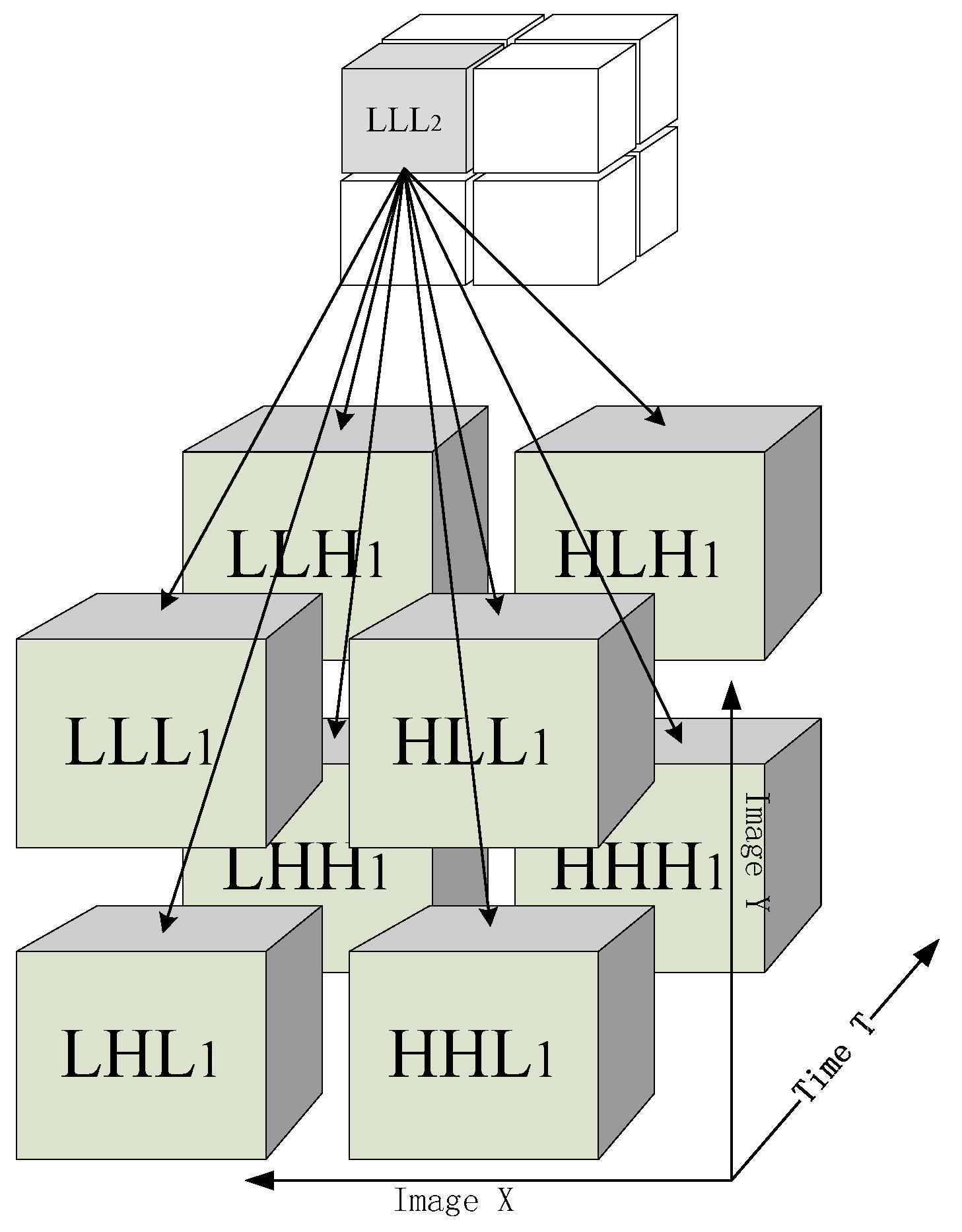
2.4. HMT Based Texture Segmentation

The HMT models based Bayesian segmentation method, called HMTseg, has been proposed in [11,13]. The HMTseg method makes use of the wavelet domain HMT model to characterize the statistical behavior of an image at multiple scales, in which the dependence among wavelet coefficient is further explored. Meanwhile, the class labels are determined by using the contex-based multiscale fusion. The segmentation method consists of three steps, raw maximum likelihood segmentation, context-based multiscale fusion, and pixel-level segmentation.

2.4.1. Raw Maximum Likelihood Segmentation

It uses the maximum likelihood (ML) classification to partition the dyadic square $d_i$ as follows:

$${\widehat{c}}_i^{ML}:=\text{arg}\underset{\mathrm{c}\in \left\{1,2,\cdots ,N_c\right\}}{\text{max}}f\left(d_i|{ℳ}_c\right)$$

(5)

${ℳ}_c$ is the parameter set for the c-th texture class. $N_c$ is the total numer of the texture classes. The square $d_i$ consists of triple wavelet coefficient tree $\{{\mathcal{T}}_i^{LH},{\mathcal{T}}_i^{HL},{\mathcal{T}}_i^{HH}\}$, in which, for example, ${\mathcal{T}}_i^{HH}$ is shown in Figure 3. Supposing each sub-band is mutual independence, there is:

$$f(d_i|{ℳ}_c)=f({\mathcal{T}}_i^{LH}{|\mathrm{\Theta }}_c^{LH}) f({\mathcal{T}}_i^{HL}{|\mathrm{\Theta }}_c^{HL})f({\mathcal{T}}_i^{HH}{|\mathrm{\Theta }}_c^{HH})$$

(6)

For each of the subtree, the likelihoods $f\left({\mathcal{T}}_i|\mathrm{\Theta }\right)$ of all dyadic squares can obtain by using the calculated conditional likelihood $f\left({\mathcal{T}}_i| S_i=m,\mathrm{\Theta }\right)$ as follows:

$$f\left({\mathcal{T}}_i|\mathrm{\Theta }\right)={\displaystyle \sum _{m=1}^M}f\left({\mathcal{T}}_i| S_i=m,\mathrm{\Theta }\right)p\left(S_i=m|\mathrm{\Theta }\right)$$

(7)

in which $p\left(S_i=m|\mathrm{\Theta }\right)$ is hidden state probability for $S_i=m$ when given the parameter $\mathrm{\Theta }$.

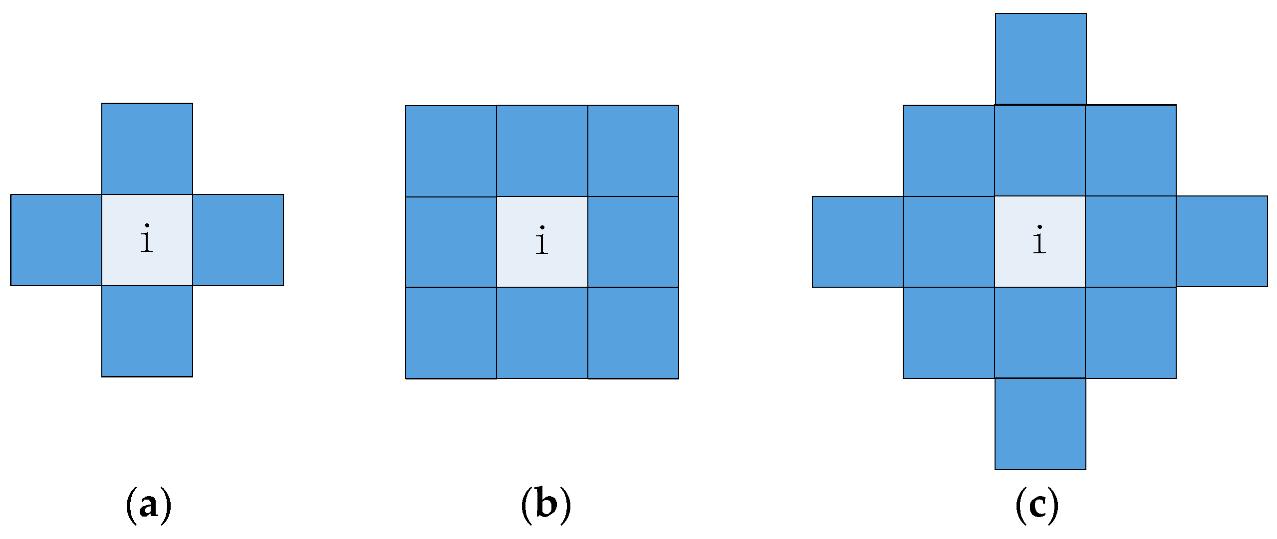
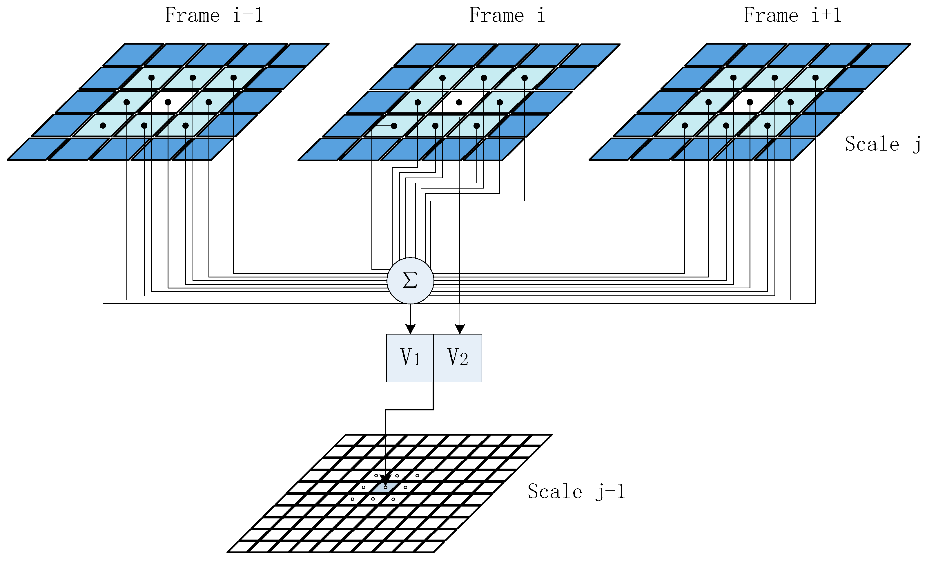
2.4.2. Context-Based Multiscale Fusion

Due to the intrinsic property of the quadtree of the wavelet transform, if the coefficient at scale j is classified to class c, it is quite likely that it four children coefficients belong to the same class. The raw segmentation can be improved by considering the dependencies between the class decisions at different scales. Therefore, Choi [13] constructs the context labeling tree and fuse the interscale information with EM algorithm. Assuming that the class labels $c^{j+1}$ at the scale j + 1 have been determined, the collection of all contexts at scale j, $v_j$, is defined as the function of $c^{j+1}$. Choi [13] has employed a simplified context tree: each $v_i^j$ at scale j will receive information from the parent label plus the parent’s eight nearest neighbors at scale j + 1. Specifically, each $v_i^j$ contains two entries, the class label of the parent and the majority vote of the class labels of the parent plus its eight neighbors. Then, a Markov chain model $v_i^j\to c_i^j\to d_i^j$ is built, and the multiscale information fusion can be realized by using the EM algorithm for context labeling tree.

2.4.3. Pixel-Level Segmentation

Because the size of a sub-band is one quarter of the original image, it requires a model for the pixel brightness of each texture image to complete the final segmentation. The original HMTseg method fits a nonzero mean Gaussian mixture distribution to the pixel values for each training texture and estimates the parameters with EM algorithm [23]. At the final level segmentation, the likelihood of each pixel is computed and the labels dependence between the finest scale level and the pixel level is the same as that of the context-based multiscale fusion stage.

3. LMM-HMT Based Description of Texture

3.1. LMM Based HMT Model

For any given set of wavelet coefficients, the two-state, zero-mean Gaussian mixture model may not provide a fit to $f_W\left(w\right)$ with the desired fidelity, we may improve accuracy by increasing the number of hidden states and allowing nonzero mean, but this also increases the computational complexity and becomes less robust accordingly [10]. To match the non-Gaussian nature of the wavelet coefficients of a texture more precisely and effectively, we utilize a mixture of Laplacian distribution instead of Gaussian mixture density. LMM can guarantee being peakier in the center and having heavier tails with least state variables, which fit the pdf of wavelet coefficients better than GMM, as shown in Figure 1. As GMM based HMT model, each coefficient is assigned with a hidden state variable $S_i=m,m\in \left\{0,1\right\},$ state 0 corresponds to the Laplace function with zero mean and small value of the scale parameter, while state 1 corresponds to the Laplace function with zero mean and large value of the scale parameter. The Laplace probability density functions of each coefficient $w_i$ in state $S_i$ can be expressed as:

$$f\left(w_i|S_i=m\right)=l\left(w_i;0,b_m\right)=\frac{1}{2b_m}\text{exp}\left(-\frac{\left|w_i\right|}{b_m}\right)$$

(8)

Therefore, an LMM-HMT model is specified in terms of the following parameters:

• The probability of the state $m$ at the root node in the coarsest scale $p_{s_1}\left(m\right);$
• The state transition probability is:

  $${\mathsf{\epsilon }}_{i,\rho \left(i\right)}^{m,n}=p_{S_i|S_{{\rho }_{\left(i\right)}}}\left(S_i=m|S_{{\rho }_{\left(i\right)}}=n\right).$$

  It is the conditional probability that $S_i$ is in state $m$ given $S_{{\rho }_{\left(i\right)}}=n,$ state variable $S_{{\rho }_{\left(i\right)}}$ is the parent state of $S_i$;
• The scale parameter $b_{i,m}$, given $S_i=m$.

We can also group these parameters for a sub-tree into a model parameter set $\mathrm{\Theta }=\left\{p_{s_1}\left(m\right),{\mathsf{\epsilon }}_{i,\rho \left(i\right)}^{m,n},b_{1,m},b_{i,m}|m,n=0,1;i=2,\cdots ,P\right\}$ (P is the number of wavelet coefficients of the sub-tree), and the LMM-HMT model of a texture that belongs to class c is parameterized by ${ℳ}_c=\left\{{\mathrm{\Theta }}_c^{LH},{\mathrm{\Theta }}_c^{HL},{\mathrm{\Theta }}_c^{HH}\right\}$ as the GMM-HMT model.

3.2. Parameter Estimation

In [10], Crouse introduced an Upward-Downward method based on the EM algorithm for estimating parameters of the HMT model. This algorithm used ML estimation of Gaussian mixture means and variances for the leaves of the tree instead of ML estimation of probability mass function (pmf) values in classical EM algorithm. According the parameters estimation framework, the parameters of the LMM-HMT model with two hidden states and the zero-mean Laplace mixture distribution are estimated by using EM algorithm.

For a single wavelet tree of a sub-band, we can make use of the Upward-Downward method [10] and the probability density distribution Equation (7) to obtain the desired conditional probabilities:

$$p\left(S_i=m|w,\mathrm{\Theta }\right)=\frac{p\left(S_i=m,{\mathcal{T}}_{1\backslash i}|\mathrm{\Theta }\right)f\left({\mathcal{T}}_i|S_i=m,\mathrm{\Theta }\right)}{{\sum }_{n=1}^{M}p\left(S_i=n,{\mathcal{T}}_{1\backslash i}|\mathrm{\Theta }\right)f\left({\mathcal{T}}_i|S_i=n,\mathrm{\Theta }\right)}$$

(9)

$$p\left(S_i=m,S_{{\rho }_{\left(i\right)}}=n|w,\mathrm{\Theta }\right)=\frac{f\left({\mathcal{T}}_i|S_i=m,\mathrm{\Theta }\right){\mathsf{ϵ}}_{i,\rho \left(i\right)}^{mn}p\left(S_{\rho \left(i\right)}=n,{\mathcal{T}}_{1\backslash i}|\mathrm{\Theta }\right)f\left({\mathcal{T}}_{\rho \left(i\right)\backslash i}|S_{\rho \left(i\right)}=n,\mathrm{\Theta }\right)}{{\sum }_{n=1}^{M}p\left(S_i=n,{\mathcal{T}}_{1\backslash i}|\mathrm{\Theta }\right)f\left({\mathcal{T}}_i|S_i=n,\mathrm{\Theta }\right)}$$

(10)

with the current parameters, where ${\mathcal{T}}_{1\backslash i}$ is the set of wavelet coefficients obtained by removing the subtree ${\mathcal{T}}_i$ from the entire wavelet coefficient tree ${\mathcal{T}}_1$. ${\mathcal{T}}_1$ includes the whole wavelet coefficients in the wavelet tree. $p(·)$ is used to denote the probablility.

At the E step of the EM algorithm, we apply the Upward-Downward method to each wavelet coefficient tree, and get the probabilities $p(S_i^k=m|w_i^k,{\mathrm{\Theta }}_l)$ and $p(S_i^k=m,S_{\rho \left(i\right)}^k=n|w_i^k,{\mathrm{\Theta }}_l)$ with the current parameters ${\mathrm{\Theta }}_l$. Then, in the M step, the parameters are re-estimated with K wavelet trees as follows:

$$p_{S_i}\left(m\right)=\frac{1}{K}{\displaystyle \sum _{k=1}^K}p\left(S_i^k=m|w_i^k,{\mathrm{\Theta }}_l\right)$$

(11)

$${\mathsf{ϵ}}_{i,\rho \left(i\right)}^{mn}=\frac{{\sum }_{k=1}^{K}p\left(S_i^k=m,S_{\rho \left(i\right)}^k=n|w_i^k,{\mathrm{\Theta }}_l\right)}{K{p}_{S_{\rho \left(i\right)}}\left(n\right)}$$

(12)

$$b_{i,m}=\frac{{\sum }_{k=1}^K\left|w_i^k\right|p\left(S_i^k=m|w_i^k,{\mathrm{\Theta }}_l\right)}{K{p}_{S_i}\left(m\right)}$$

(13)

As stated in [13], we also use the intra-tying for the parameter estimation of each HMT, that is to say, the same state transition probabilities and mixture scale parameters are used for all wavelet coefficients at the same scale. The complete parameter set of LMM-HMT model is estimated by applying the tree-structure EM algorithm to, for example, LH, HL and HH directional sub-bands of an image texture.

3.3. Pixel-Level Texture Description

After the raw segmentation with the wavelet-domain LMM-HMT models and the multiscale fusion, the pixel-level segmentation is necessary to obtain final result completely. In this paper, the pixel values are considered as the realizations of a random variable that obeys a Laplace mixture distribution instead of a Gaussian mixture. In order to describe the region property of the texture, the multivariate Laplace mixture distribution is used.

The Laplace distribution belongs to the exponential power distribution family. The density function of the multivariate exponential power (MEP) distributions is defined as [24]:

$$ℳℰ𝒫(x|\mu ,\mathrm{\Sigma },\mathsf{\kappa })=ℂ{\left|\mathrm{\Sigma }\right|}^{-\frac{1}{2}}\text{exp}\{-\frac{1}{2}{[{(x-\mu )}^T{\mathrm{\Sigma }}^{-1}(x-\mu )]}^{\frac{\kappa }{2}}\}$$

(14)

where $\mathsf{\mu }\in {ℝ}^d,\mathrm{\Sigma }\in {ℝ}^{d\times d}$ (a symmetric positive definite matrix) and:

$$ℂ=\frac{d\mathrm{\Gamma }\left(\frac{d}{2}\right)}{{\pi }^{\frac{d}{2}}\mathrm{\Gamma }\left(1+\frac{d}{\kappa }\right)2^{1+\frac{d}{\kappa }}}$$

(15)

$\mathrm{\Gamma }$ is Gamma Function. $d\in \mathbb{N}$ presents the dimension. The shape of a MEP is strongly influenced by parameter $\kappa$, when $\kappa =2,$ it is actually a Gaussian distribution; when $\kappa =1,$ it becomes the multivariate Laplace distribution:

$$p\left(x|\mu ,\mathrm{\Sigma }\right)=\frac{d\mathrm{\Gamma }\left(\frac{d}{2}\right)}{{\pi }^{\frac{d}{2}}\mathrm{\Gamma }\left(1+d\right)2^{1+d}}{\left|\mathrm{\Sigma }\right|}^{-\frac{1}{2}}\text{exp}\left\{-\frac{1}{2}{[{\left(x-\mu \right)}^T{\mathrm{\Sigma }}^{-1}\left(x-\mu \right)]}^{\frac{1}{2}}\right\}$$

(16)

which is a generalized version of Equation (1). Therefore, the multivariate Laplace mixture distribution is:

$$p\left(x|\mathrm{\Omega }\right)={\displaystyle \sum _{m=1}^M}{\omega }_m p_m\left(x{|\mathrm{\Omega }}_m\right)$$

(17)

with the parameter set $\mathrm{\Omega }=\left\{{\omega }_1,\cdots ,{\omega }_M,{\mu }_1,\cdots ,{\mu }_M,{\mathrm{\Sigma }}_1,\cdots ,{\mathrm{\Sigma }}_M\right\}$. Here, ${\mathrm{\Omega }}_m=\left\{{\mu }_m,{\mathrm{\Sigma }}_m\right\}$ is the parameter of the m-th Laplace density function of the mixture distribution. ${\omega }_m$ is the weight value, and ${\sum }_{m=1}^M{\omega }_m=1$. x is a vector. For each pixel i of a texture, a vector can be constructed by accumulating this pixel and its neighbors that is shown in Figure 4. The resulting vectors of the texture are modeled with the multivariate Laplace mixture distribution to describe the texture for the pixel level segmentation. If only the pixel i is considered, this mixture distribution becomes a scalar distribution. In generally, the large neighborhood includes more pixels, so we can obtain the better description of the texture. However, the small neighborhood is useful to accurately locate the boundary of different textures. Therefore, in this paper, we utilize the second order neighbor system as shown in Figure 4b.

Given a data set $\mathcal{X}=\left\{x_1,\cdots ,x_N\right\}$, the log-likelihood for the mixture distribution is given by:

$$ℒ\left(\mathrm{\Omega }|\mathcal{X}\right)=ln\left({\displaystyle \prod _{n=1}^N}p\left(x_n|\mathrm{\Omega }\right)\right)={\displaystyle \sum _{n=1}^N}ln\left({\displaystyle \sum _{m=1}^M}{\omega }_m p_m\left(x_n{|\mathrm{\Omega }}_m\right)\right)$$

(18)

where $p_m\left(x_n{|\mathrm{\Omega }}_m\right)$ follows multivariate Laplace distribution, and $x_n$ is the vector formed from the texture. Sascha [24] has estimated the parameters of the mixture of MEP distributions by using EM algorithm. Because multivariate Laplace distribution is a special case ($\kappa =1$ in Equation (16)) of the MEP distribution, we can easily obtain the estimated parameters as follows:

$${\omega }_m=\frac{1}{N}{\displaystyle \sum _{n=1}^N}{p}_{nm}$$

(19)

$${\mu }_m=\frac{{\sum }_{n=1}^N{p}_{nm}{\zeta }_{nm}^{-1/2}{x}_n}{{\sum }_{n=1}^N{p}_{nm}{\zeta }_{nm}^{-1/2}}$$

(20)

$${\mathrm{\Sigma }}_m=\frac{{\sum }_{n=1}^N{p}_{nm}{\zeta }_{nm}^{-1/2}{\gamma }_{nm}}{2{\sum }_{n=1}^N{p}_{nm}}$$

(21)

with:

$${\zeta }_{nm}={\left(x_n-{\mu }_m\right)}^T{\mathrm{\Sigma }}_m^{-1}\left(x_n-{\mu }_m\right)$$

(22)

$${\gamma }_{nm}=\left(x_n-{\mu }_m\right){\left(x_n-{\mu }_m\right)}^T$$

(23)

$$p_{nm}=p\left(k|x_n,{\mathrm{\Omega }}_m\right)=\frac{{\omega }_m p_m\left(x_n{|\mathrm{\Omega }}_m\right)}{{\sum }_{j=1}^M{\omega }_j p_j\left(x_n{|\mathrm{\Omega }}_j\right)}$$

(24)

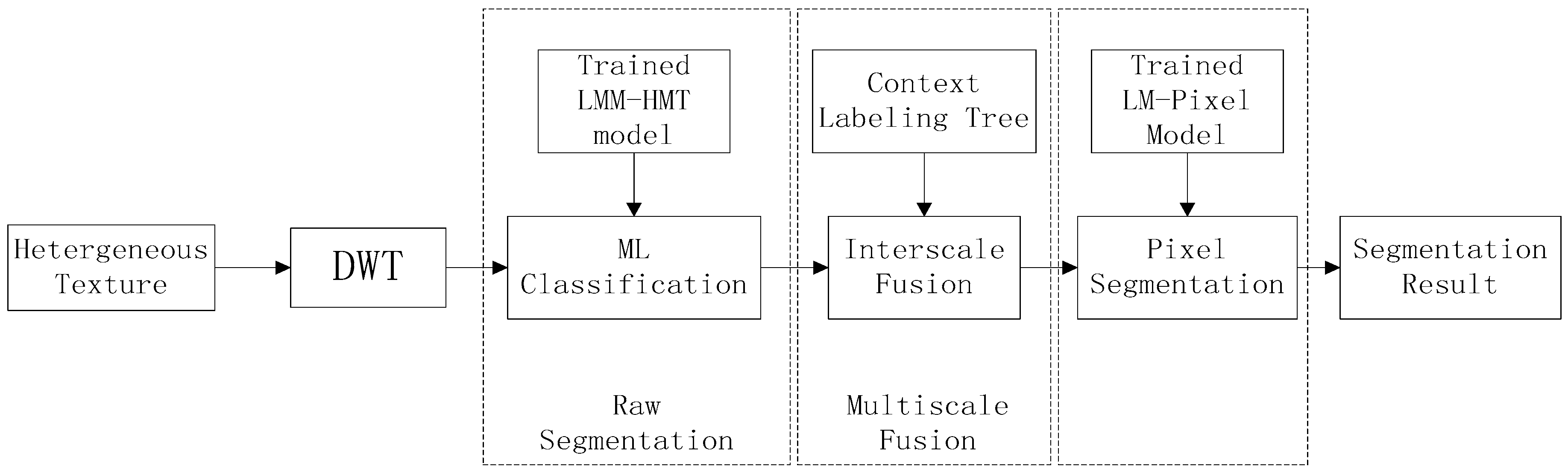
4. Texture Segmentation

After training the wavelet domain LMM-HMT model and pixel-level Laplace mixture distribution model for a homogeneous (image or dynamic) texture, we can use them to segment the heterogeneous texture. As mentioned in Section 2.4, the segmentation method includes three steps, raw maximum likelihood segmentation, context-based multiscale fusion, and pixel-level segmentation, which is shown in Figure 5. The differences between our method and HMTseg [13] are just the marginal distribution of HMT model and the pixel-level description. The implementation is summarized as follows.

(1)

Model training. For each texture class, we train the wavelet domain LMM-HMT model with the homogeneous texture samples by using EM algorithm as the Section 3.2, and obtain the model parameters ${ℳ}_c$, in which c denotes the cth texture class. Meanwhile, the pixel-level multivariate Laplace mixture model parameters are gotten with Equations (19)–(24).

(2)

Raw maximum likelihood segmentation. For a heterogeneous texture to be segmented, the likelihood of each subtree at different scale can be computed by using the HMT likelihood computation method and the Equation (7). The raw segmentation $c^J$ at the coarest scale is accomplished by using Equation (5) with the trained LMM-HMT model parameters ${ℳ}_c$.

(3)

Context-based multiscale fusion. At the scale j, the context vectors $v_i^j$s are constructed from the segmentation label $c^{j+1}$ at scale j + 1. The segmentation result $c^j$ is obtained by using EM algorithm and maximizing the contextual posterior distribution as the work [13].

(4)

Pixel-level segmentation. Compute the likelihood of each pixel with the trained pixel-level multivariate Laplace mixture models. Perform the context-based fusion scheme from the scale j = 1 to the pixel-level as the step (3). The output is the final segmentation result.

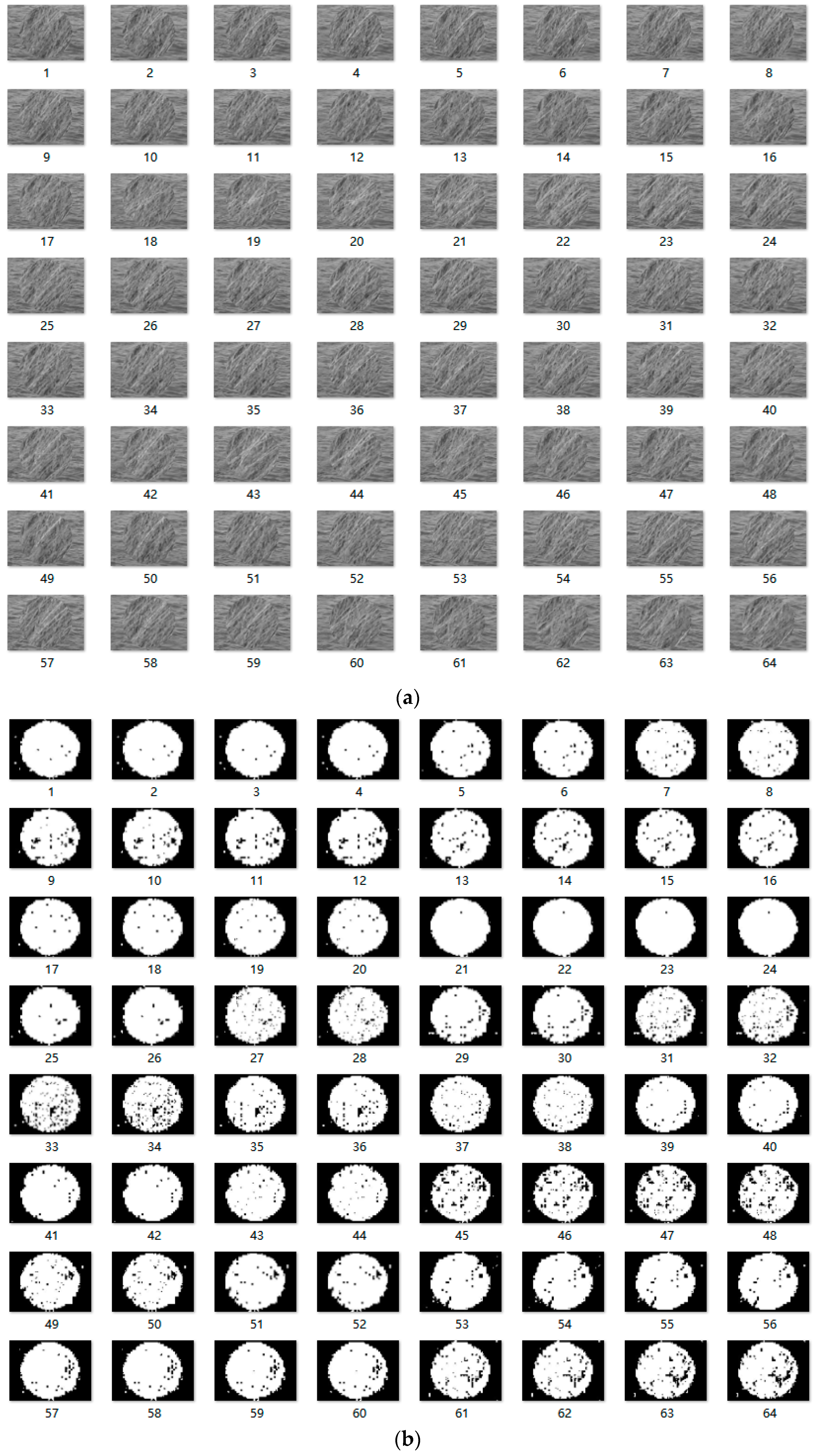
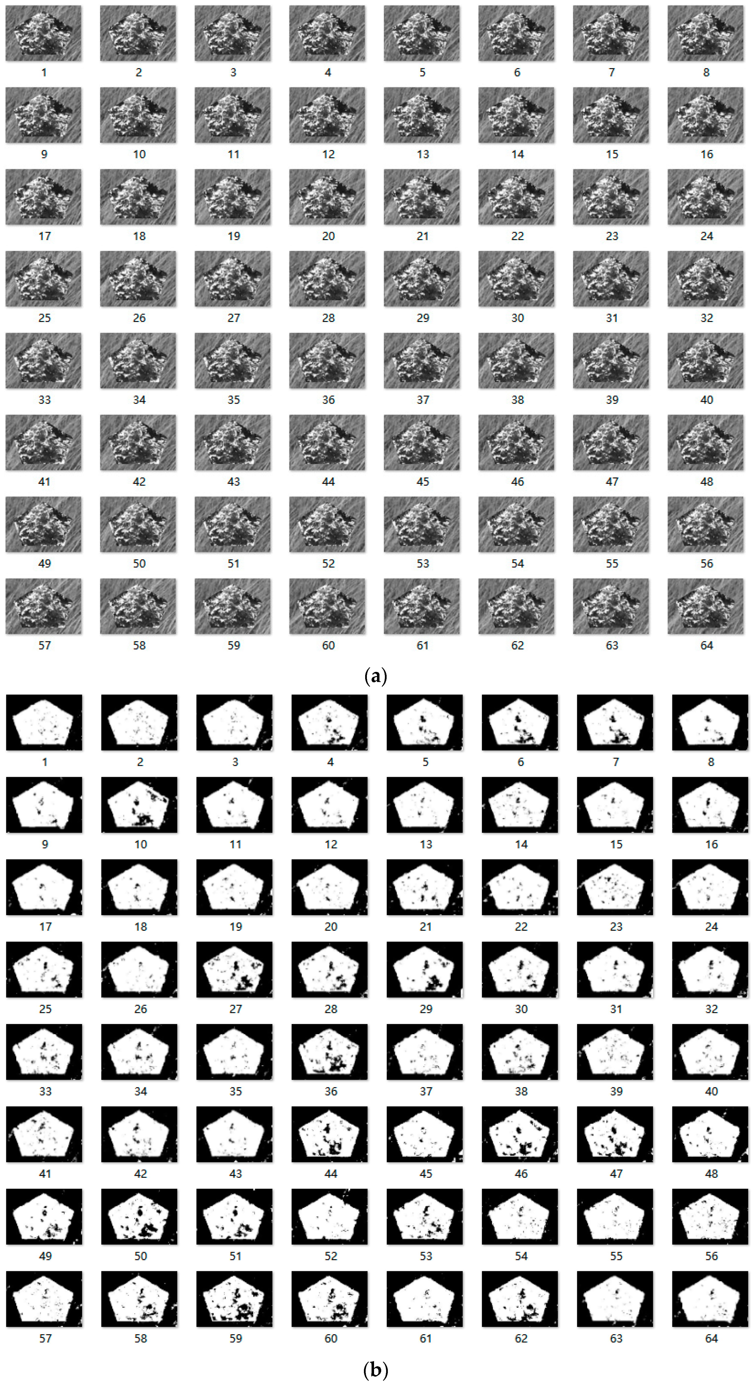
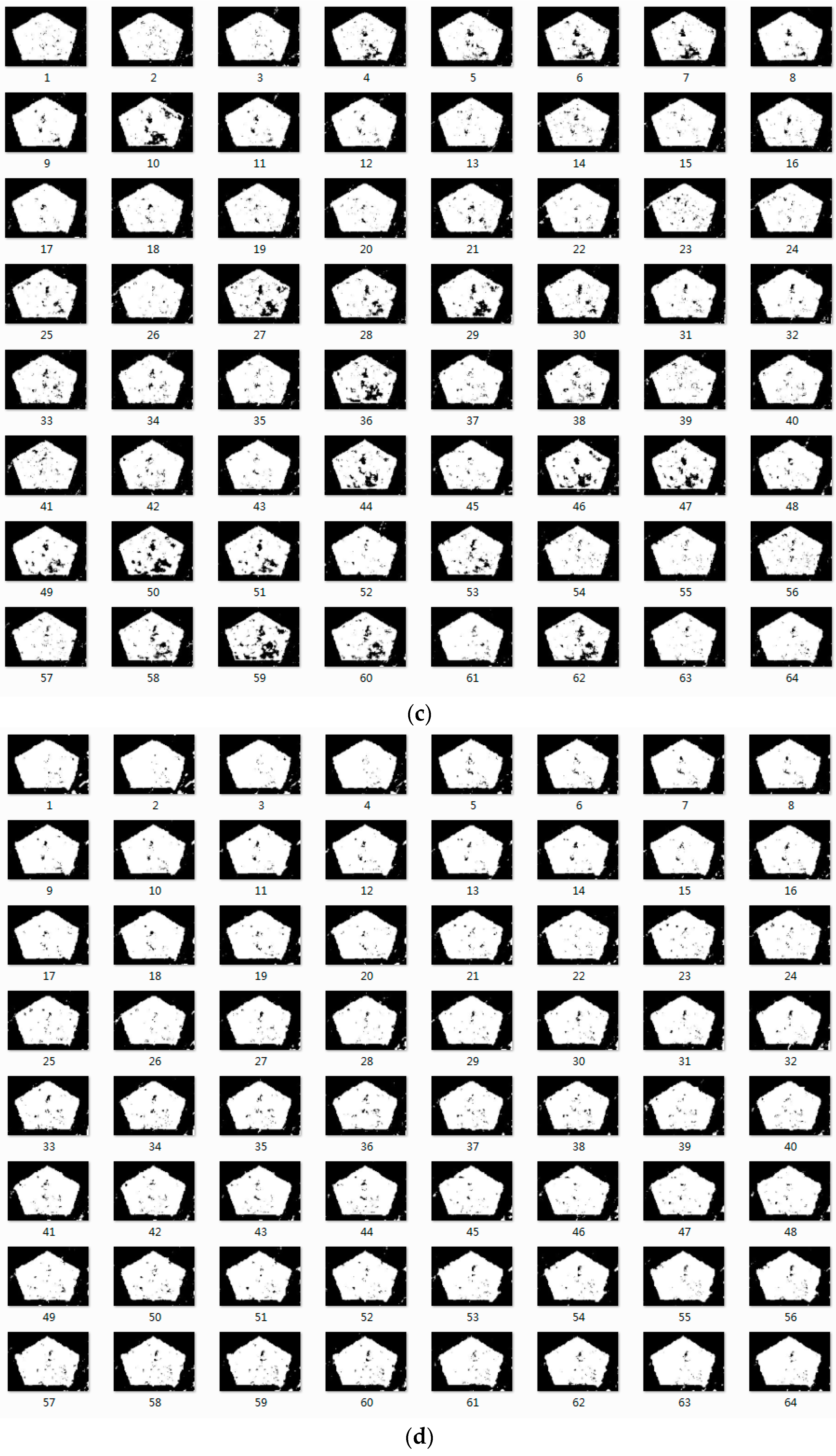
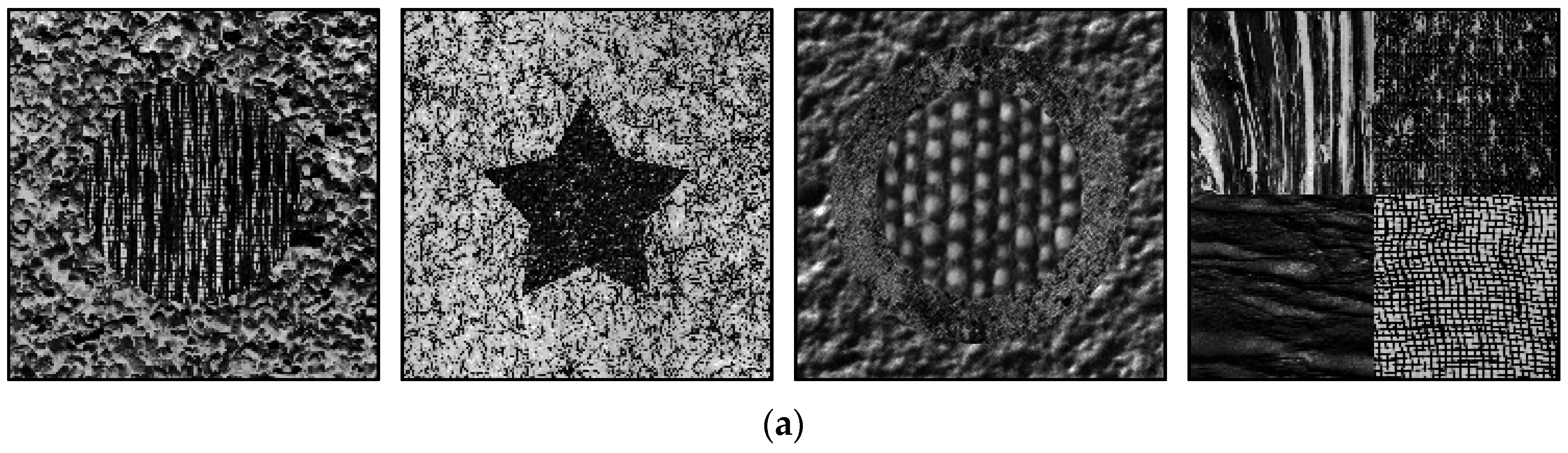
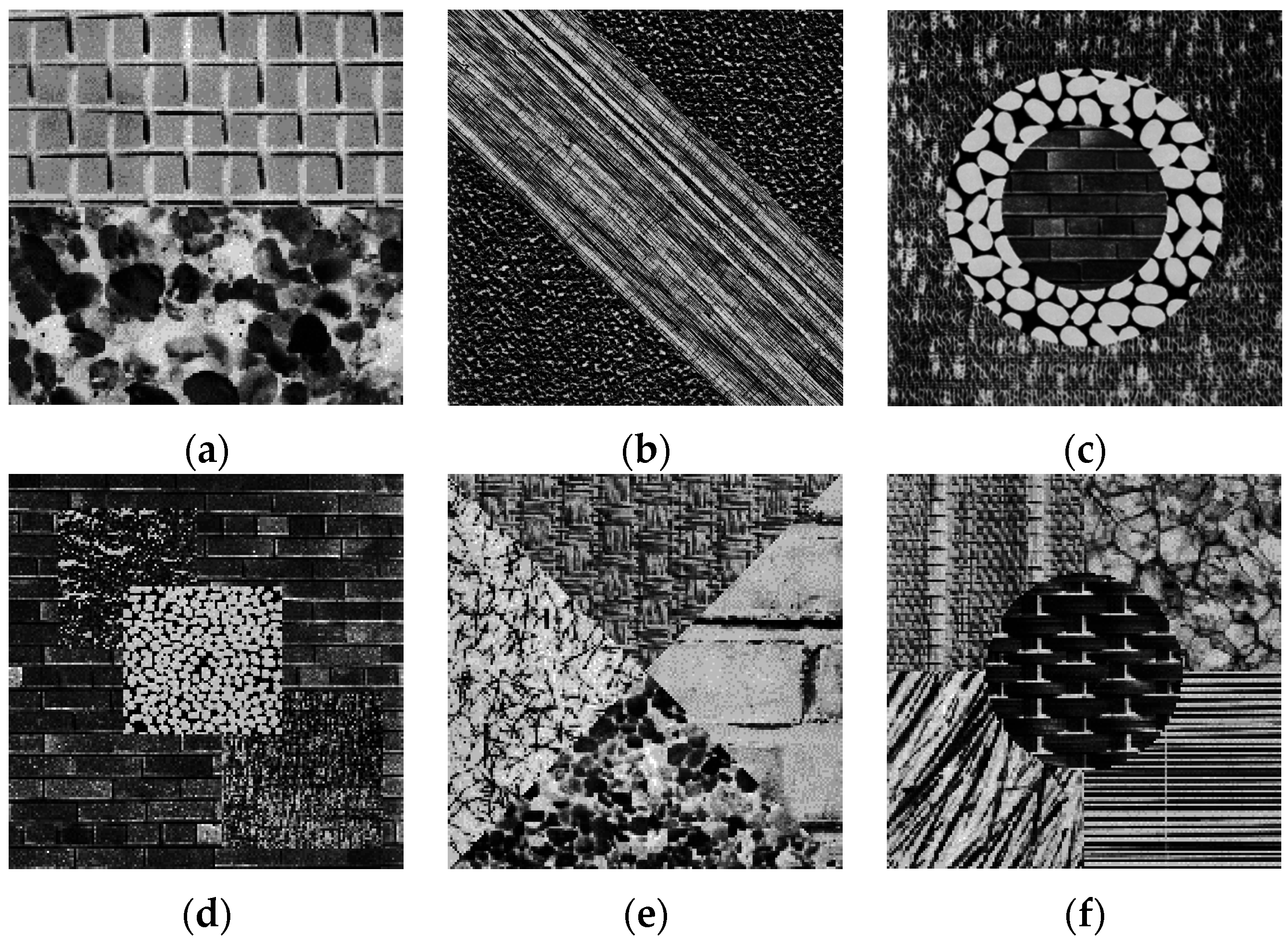
4.1. Image Texture Segmentation

The HMT model based segmentation method HMTseg and its improved versions have been applied in document image segmentation, aerial imagery segmentation and texture segmentation. Taking the texture property into account, we use the wavelet domain LMM-HMT model and Laplace mixture distribution model to describe the texture. Therefore, at the training stage, their parameters should be estimated with the Equations (11)–(13) and Equations (19)–(24), respectively. Then the method shown in Figure 5 is utilized to segment the homogeneous image texture.

4.2. Dynamic Texture Segmentation

As mentioned in the introduction section, dynamic textures are video sequences of complex dynamical objects. Dynamic texture segmentation addresses the problem of decomposing an image sequence into a collection of homogeneous texture regions. The introduced dynamic texture segmentation is based on spatial-temporal wavelet domain LMM-HMT and pixel-level multivariate Laplace mixture distribution model.

For 2-D wavelet transform, each low-frequency sub-band is decomposed into four sub-bands, one approximate sub-band and three detail sub-bands, which leads naturally to a quad-tree structure on the wavelet coefficients. Therefore, 2-D HMT model is formed as shown in Figure 3. However, for the spatial-temporal wavelet transform, each level transform results in one approximate sub-band and seven detail sub-bands as shown in Figure 6, from which the octree structure is formed. That is to say, each parent node is connected to its eight child wavelet coefficents. Therefore, there are seven parallel octree structures. The complete LMM-HMT model consists of seven LMM-HMT models, where each of them corresponds to one sub-band. The LMM-HMT model for the dynamic texture uses Markov chain to model the interscale dependences and the Laplace mixture distribution to characterize the wavelet coefficient. Then the LMM-HMT model is parameterized by $ℳ=\left\{{\mathrm{\Theta }}^{LLH},{\mathrm{\Theta }}^{LHL},{\mathrm{\Theta }}^{LHH},{\mathrm{\Theta }}^{HLL},{\mathrm{\Theta }}^{HLH},{\mathrm{\Theta }}^{HHL},{\mathrm{\Theta }}^{HHH}\right\}$, where each parameter subset of $ℳ$ is for a sub-band (For example, ${\mathrm{\Theta }}^{LLH}$denotes the parameter set of sub-band LLH). For tractability reasons, we assume that the seven sub-bands of the spatial-temporal wavelet domain are statistically independence. Then for a dynamic texture belonging to class c, we can estimation the parameters for each sub-band with EM algorithm (Equations (11)–(13)), and obtain ${ℳ}_c=\left\{{\mathrm{\Theta }}_c^{LLH},{\mathrm{\Theta }}_c^{LHL},{\mathrm{\Theta }}_c^{LHH},{\mathrm{\Theta }}_c^{HLL},{\mathrm{\Theta }}_c^{HLH},{\mathrm{\Theta }}_c^{HHL},{\mathrm{\Theta }}_c^{HHH}\right\}$ of the complete LMM-HMT model.

The general segmentation method based on LMM-HMT model is shown in Figure 5. It is easy to extend LMM-HMT model based image texture segmentation method to the spatial-temporal wavelet domain LMM-HMT model based dynamic texture segmentation. We should put emphasis on the context labeling tree at the context-based interscale fusion stage. In this paper, the context labeling tree is constructed as shown Figure 7. The state of a wavelet coefficient at scale j − 1 is dependent on its parent plus eight neighbors and the states of the coefficients of the adjacent frames at scale j. Thus, context vector $v^{j-1}$ is formed by accumulating the parent and the majority vote of all other 26 neighbors. Then, this context vector is used at the multiscale fusion stage.

5. Experimental Results

In order to evaluate the texture segmentation method based on the wavelet domain LMM-HMT model, we conduct the experiments on image texture segmentation and dynamic texture segmentation in this section. The synthetic textures are used as the exprimental materials, and the segmentation performance is determined by comparing the segmentation results and the ground truths. Specifically, we quantify the performance of texture segmentation by the percentage of pixels which are correctly segmented, it’s also called accuracy rate:

$$accuracy=\frac{N_{correct}}{N}\times 100\%$$

(25)

where $N_{correct}$ is the number of correctly segmented pixels, $N$ is the total pixel number of texture.

5.1. Image Texture Segmentation

The experimental heterogeneous texture images IT1–IT4 are shown in Figure 8a, which are synthesized with the Brodatz textures [25] and the ground truths. Firstly, we make use of 3-level Daubechies-1 wavelet transform, and then construct and train the LMM-HMTs (GMM-HMTs). Then we segment the texture images with the proposed method. The results are shown in Figure 8f. The segmentation results in Figure 8c are obtained by using GMM-HMT and GM model for pixel-level segmentation, while results in Figure 8d are obtained by using LMM-HMT and GM model for pixel level. The segmentation accuracy rates are listed in

Table 1. Image texture segmentation performance comparison (accuracy rate: %).

Texture	GMM-HMT	LMM-HMT	Factorization [8]	LMM-HMT with LM-Pixel
IT1	95.17	95.34	97.52	96.21
IT2	96.56	97.29	96.80	97.42
IT3	94.32	94.65	92.43	95.04
IT4	96.01	96.23	95.23	96.37

. It is demonstrated that the proposed method is better than wavelet domain GMM-HMT model based method.

In order to further test the performance of the introduced method, we also conduct other experiments on several synthetic image textures IT5–IT10 as shown in Figure 9. The accuracy rates of different segmentation methods are listed in

Table 2. Image texture segmentation results (accuracy rate: %).

Texture	GMM-HMT	LMM-HMT with LM-Pixel
IT5	93.55	94.74
IT6	93.64	93.82
IT7	93.37	93.56
IT8	95.44	94.79
IT9	90.28	89.14
IT10	65.29	66.73

, we can see that the method using LMM-HMT model performs better than general HMT algorithm in average.

5.2. Dynamic Texture Segmentation

The dynamic texture segmentation experiments are conducting on the synthesized videos that are constructed with the dyanmic textures of the DynTex dataset [26,27]. All videos consist of 64 frames, and the size of each frame is 176 × 168. The 3-level Daubechies-1 spatial-temporal wavelet transform is used to form the LMM-HMT model for describing the dynamic texture. For the multiscale fusion, we utilize the spatial-temporal parent neighbors (as shown in Figure 7) to construct the context labeling tree. The segmentation is implemented with the method mentioned in fourth section.

The three adjacent frames selected from a synthesized video consisting of two dynamic textures are shown in Figure 10a. After the raw segmentation and multiscale fusion stages, Figure 10b is the result by using the context labeling tree based on the ordinary spatial second-order neighbors (eight neighbors), while Figure 10c is the result by utilizing spatial-temporal parent neighbors based context labeling tree. It is can be seen that the segmentation accuracy rates has been improved.

We also verify the segmentation performance with different synthetic videos in Figure 11, Figure 12 and Figure 13. Each figure includes the original video (64 frames) to be segmented, the segmentation results by using the GMM-HMT and GM model based method, LMM-HMT and GM model based method, and LMM-HMT and LM model based method. The accuracy rate of each frame is calculated. The results are summarized in

Table 3. Dynamic texture segmentation results (accuracy rate: %).

Texture	GMM-HMT			LMM-HMT
				GM-Pixel			LM-Pixel
	Max	Min	Avg	Max	Min	Avg	Max	Min	Avg
DT1	97.41	92.97	94.92	97.29	91.52	96.11	97.45	93.56	96.43
DT2	97.33	90.31	95.23	96.57	95.43	95.96	96.85	96.24	96.31
DT3	98.14	94.98	97.19	98.92	94.85	97.06	98.78	95.80	97.63

, in which “Max”, ”Min” and “Avg” denote the maximum, minimum and average segmentation accuracy rates of all frames, respectively. The introduced method shows potential for the dynamic texture segmentation.

6. Conclusions

In this paper, we introduce a wavelet domain HMT model fitting by a Laplacian mixture distribution instead of Gaussian conditions, from which the texture segmentation method is derived. Specifically, we make use of a LMM-HMT model to describe the wavelet coefficients and their interscale dependence, and the multivariate Laplacian mixture distribution to characterize the pixel values for pixel-level segmentation. For the dynamic texture segmentation, we also utilize the spatial-temporal parent neighbors to construct the context labeling tree, so as to improve the segmentation during multiscale fusion stage. The segmentation experiments are conducted on the image textures and dynamic textures, from which the performance of the proposed method is verified. The image texture analysis and applications based on the wavelet domain hidden Markov tree model have been intensively investigated in past years. This paper also tries to solve the dynamic texture segmentation problem by using the wavelet domain hidden Markov model. However, we process the dynamic texture (spatio-temporal image sequence) as a 3D volume data, which cannot effectively capture the dynamic texture property along the temporal domain. Therefore, a different spatio-temporal wavelet decomposition, such as different decomposition levels for spatial and temporal domains, and the corresponding hidden Markov model should be one of our future works. In addition, for the dynamic texture with slow change along the temporal domain, the Haar wavelet transform may result in some special sub-bands, in which almost all coefficients approach zero. It is difficult to model these sub-bands. Another wavelet basis-based wavelet domain representation for the dynamic texture should be studied for this case.

References

1. Chen, J.; Zhao, G.Y.; Salo, M.; Rahtu, E.; Pietikainen, M. Automatic dynamic texture segmentation using local descriptors and optical flow. IEEE Trans. Image Proc. 2013, 22, 326–339. [Google Scholar] [CrossRef] [PubMed]
2. Qiao, Y.L.; Weng, L.X. Hidden Markov model based dynamic texture classification. IEEE Signal Proc. Lett. 2015, 22, 509–512. [Google Scholar] [CrossRef]
3. Wang, L.; Liu, J. Texture classification using multiresolution Markov random field models. Pattern Recognit. Lett. 1999, 20, 171–182. [Google Scholar] [CrossRef]
4. Qiao, Y.L.; Wang, F.S. Wavelet-based dynamic texture classification using Gumbel distribution. Math. Probl. Eng. 2013, 2013, 762472. [Google Scholar] [CrossRef]
5. Nelson, J.D.B.; Nafornta, C.; Isar, A. Semi-local scaling exponent estimation with box-penalty constraints and total-variation regularization. IEEE Trans. Image Proc. 2016, 25, 3167–3181. [Google Scholar] [CrossRef] [PubMed]
6. Pustelnik, N.; Wendt, H.; Abry, P.; Dobigeon, N. Combining Local Regularity Estimation and Total Variation Optimization for Scale-Free Texture Segmentation. 2015; arXiv:1504.05776. [Google Scholar]
7. Arbelaez, P.; Maire, M.; Fowlkes, C.; Malik, J. Contour detection and hierarchical image segmentation. IEEE Trans. Pattern Anal. Mach. Intell. 2011, 33, 898–916. [Google Scholar] [CrossRef] [PubMed]
8. Yuan, J.; Wang, D.; Cheriyadat, A.M. Factorization-based texture segmentation. IEEE Trans. Image Proc. 2015, 24, 3488–3496. [Google Scholar] [CrossRef] [PubMed]
9. Sasidharan, R.; Menaka, D. Dynamic texture segmentation of video using texture descriptors and optical flow of pixels for automating monitoring in different environments. In Proceedings of the International Conference on Communication and Signal Processing, Melmaruvathur, India, 3–5 April 2013; pp. 841–846.
10. Crouse, M.S.; Nowak, R.D.; Baraniuk, R.G. Wavelet-based statistical signal processing using hidden Markov models. IEEE Trans. Signal Proc. 1998, 46, 886–902. [Google Scholar] [CrossRef]
11. Romberg, J.K.; Choi, H.; Baraniuk, R.G. Bayesian tree-structured image modeling using wavelet-domain hidden Markov models. IEEE Trans. Signal Proc. 2001, 10, 1056–1068. [Google Scholar] [CrossRef] [PubMed]
12. Durand, J.B. Computational methods for hidden Markov tree models—An application to wavelet trees. IEEE Trans. Signal Proc. 2004, 52, 2551–2560. [Google Scholar] [CrossRef]
13. Choi, H.; Baraniuk, R.G. Multiscale image segmentation using wavelet-domain hidden Markov Models. IEEE Trans. Signal Proc. 2001, 10, 1309–1321. [Google Scholar] [CrossRef] [PubMed]
14. Ye, W.; Zhao, J.H.; Wang, S.; Wang, Y.; Zhang, D.Y.; Yuan, Z.Y. Dynamic texture based smoke detection using Surfacelet transform and HMT model. Fire Saf. J. 2015, 73, 91–101. [Google Scholar] [CrossRef]
15. Wang, X.Y.; Sun, W.W.; Wu, Z.F.; Yang, H.Y.; Wang, Q.Y. Color image segmentation using PDTDFB domain hidden Markov tree model. Appl. Soft Comput. 2015, 29, 138–152. [Google Scholar] [CrossRef]
16. Teodoro, A.; Bioucas-Dias, J.; Figueiredo, M. Image Restoration and Reconstruction Using Variable Splitting and Class-Adapted Image Priors. 2016; arXiv.1602.04052. [Google Scholar]
17. Hajri, H.; Ilea, I.; Said, S.; Bombrun, L.; Berthoumieu, Y. Riemannian Laplace distribution on the space of symmetric positive definite matrices. Entropy 2016, 18, 98. [Google Scholar] [CrossRef]
18. Nath, V.K.; Mahanta, A. Image denoising based on Laplace distribution with local parameters in Lapped transform domain. In Proceedings of the International Conference on Signal Processing and Multimedia Applications, Seville, Spain, 18–21 July 2011; pp. 1–6.
19. Figueiredo, M.; Bioucas-Dias, J.; Nowak, R. Majorization-minimization algorithms for wavelet-based image restoration. IEEE Trans. Image Proc. 2007, 16, 2980–2991. [Google Scholar] [CrossRef]
20. Huda, A.R.; Nadia, J.A. Some Bayes’ estimators for Laplace distribution under different loss functions. J. Babylon Univ. 2014, 22, 975–983. [Google Scholar]
21. Bishop, C.M. Pattern Recognition and Machine Learning; Springer: New York, NY, USA, 2006. [Google Scholar]
22. Dempster, A.P.; Laird, N.M.; Rubin, D.B. Maximum-likelihood from incomplete data via the EM algorithm. J. R. Stat. Soc. Ser. B 1977, 39, 1–38. [Google Scholar]
23. Song, X.M.; Fan, G.L. Unsupervised Bayesian image segmentation using wavelet-domain hidden Markov models. In Proceedings of the International Conference on Image Processing, Barcelona, Spain, 14–17 September 2003; pp. 423–426.
24. Brauer, S. A Probabilistic Expectation Maximization Algorithm for Multivariate Laplacian Mixtures. Master’s Thesis, Paderborn University, Paderborn, Germany, 2014. [Google Scholar]
25. Brodatz, P. Textures: A Photographic Album for Artists & Designers; Dover: New York, NY, USA, 1966. [Google Scholar]
26. Péteri, R.; Fazekas, S.; Huiskes, M.J. DynTex: A comprehensive database of dynamic textures. Pattern Recognit. Lett. 2010, 31, 1627–1632. [Google Scholar] [CrossRef]
27. The DynTex Database. Available online: http://dyntex.univ-lr.fr/index.html (accessed on 26 October 2016).
Figure 1. (a) “Floor” texture and (b) its wavelet coefficient histogram fitted with two-state, zero mean Gaussian mixture model (GMM) and Laplace mixture model (LMM).
Entropy 18 00384 g001
Figure 2. A Gaussian distribution and a Laplace distribution (zero mean and unit variance).
Entropy 18 00384 g002
Figure 3. 2-D hidden Markov tree (HMT) model.
Entropy 18 00384 g003
Figure 4. Neighbor system. (a) first-order 4-neighbor; (b) second-order 8-neighbor; (c) third-order 12-neighbor.
Entropy 18 00384 g004
Figure 5. The flow diagram of texture segmentation based on LMM-HMT model. As GMM-HMT base segmentation method, texture segmentation based on LMM-HMT model consists of the raw segmentation, the multiscale fusion and the pixel-level segmentation.
Entropy 18 00384 g005
Figure 6. Spatial-temporal wavelet transform. There are one approximate sub-band and seven detail sub-bands after one-level wavelet decomposition of the dynamic texture.
Entropy 18 00384 g006
Figure 7. The context labeling tree model for dynamic texture segmentation.
Entropy 18 00384 g007
Figure 8. The results of texture image segmentation using GMM-HMT and LMM-HMT. (a) Textures to be segmented; (b) Ground truths; (c) The results using GMM-HMT model and pixel-level GM model; (d) The results using LMM-HMT model and pixel-level GM model; (e) Factorization [8] (the parameters are the same as that of the Texture Mosaics in Section IV of [8]. The better results can be obtained by adjusting the parameters for different textures); (f) The results using LMM-HMT and pixel-level LM model.
Entropy 18 00384 g008aEntropy 18 00384 g008b
Figure 9. Synthetic image textures: (a) IT5; (b) IT6; (c) IT7; (d) IT8; (e) IT9; (f) IT10.
Entropy 18 00384 g009
Figure 10. Results of multiscale fusion. (a) Three adjacent frames selected from a synthesized video; (b) Results with the context labeling tree based on the ordinary spatial second-order neighbors; (c) Result with the spatial-temporal parent neighbors based context labeling tree.
Entropy 18 00384 g010
Figure 11. Segmentation experiments. (a) Textures to be segmented; (b) The results using GMM-HMT model and pixel-level GM model; (c) The result using LMM-HMT model and pixel-level GM model; (d) The result using LMM-HMT and pixel-level LM model.
Entropy 18 00384 g011aEntropy 18 00384 g011b
Figure 12. Segmentation experiments. (a) Textures to be segmented; (b) The results using GMM-HMT model and pixel-level GM model; (c) The result using LMM-HMT model and pixel-level GM model; (d) The result using LMM-HMT and pixel-level LM model.
Entropy 18 00384 g012aEntropy 18 00384 g012b
Figure 13. Segmentation experiments. (a) Textures to be segmented; (b) The results using GMM-HMT model and pixel-level GM model; (c) The result using LMM-HMT model and pixel-level GM model; (d) The result using LMM-HMT and pixel-level LM model.
Entropy 18 00384 g013aEntropy 18 00384 g013b