
Study on the Stability and Entropy Complexity of an Energy-Saving and Emission-Reduction Model with Two Delays

Abstract
:1. Introduction
2. Equilibrium Points and Local Stability
2.1. Case 1
2.2. Case 2
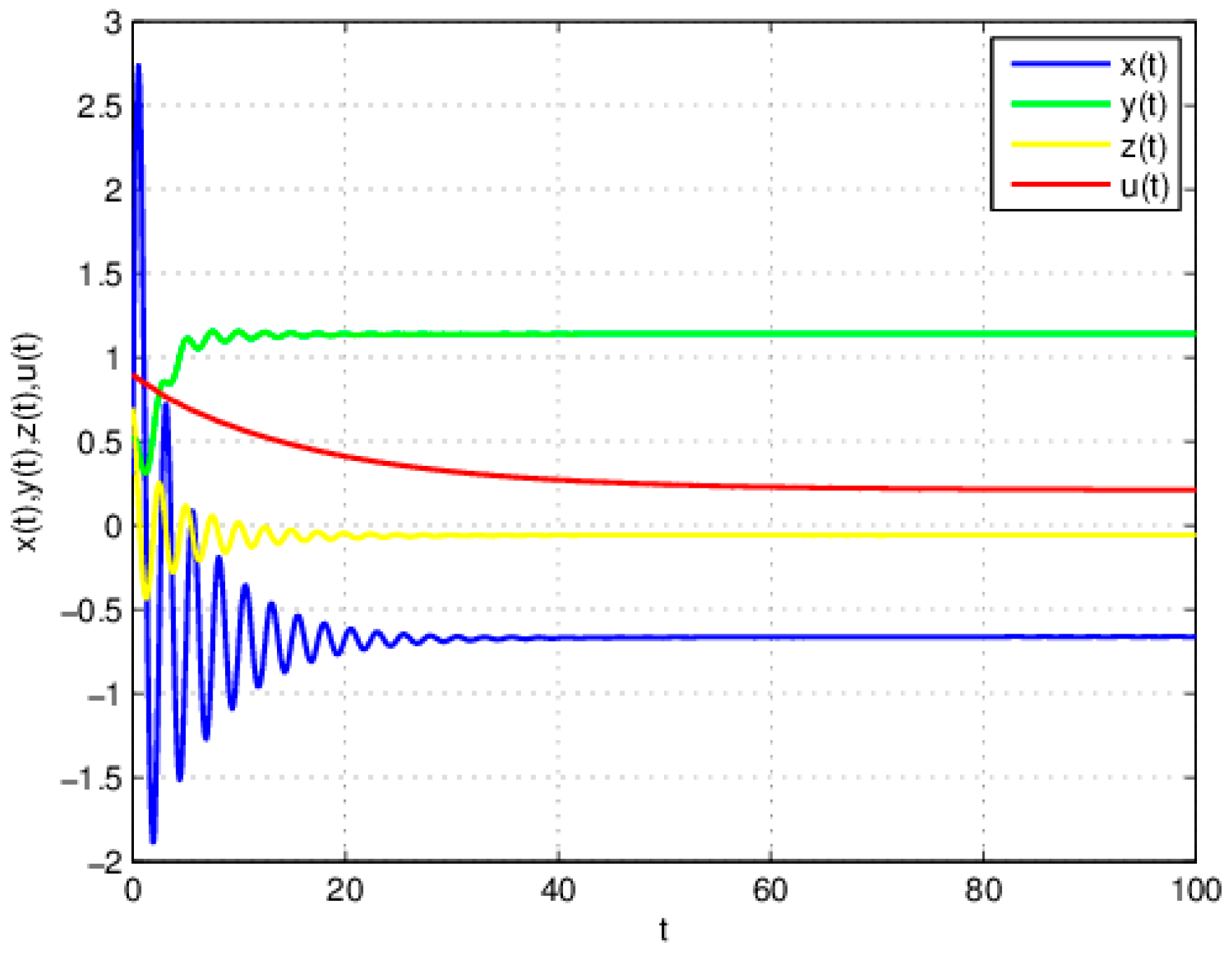
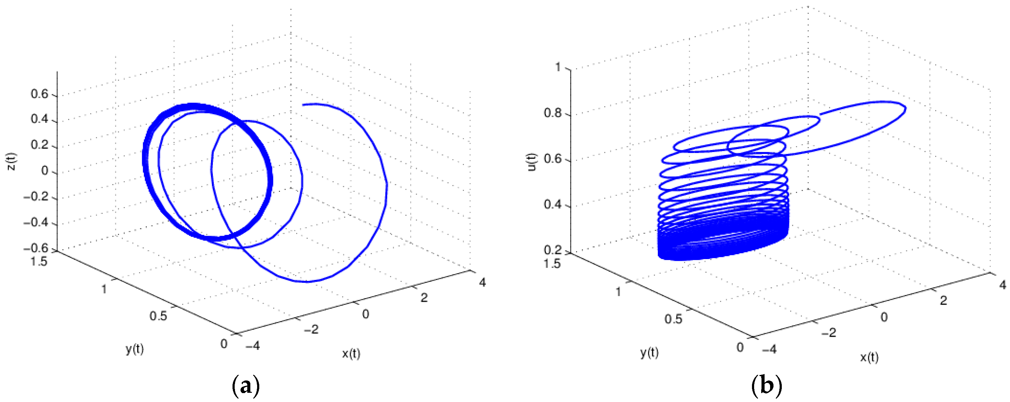
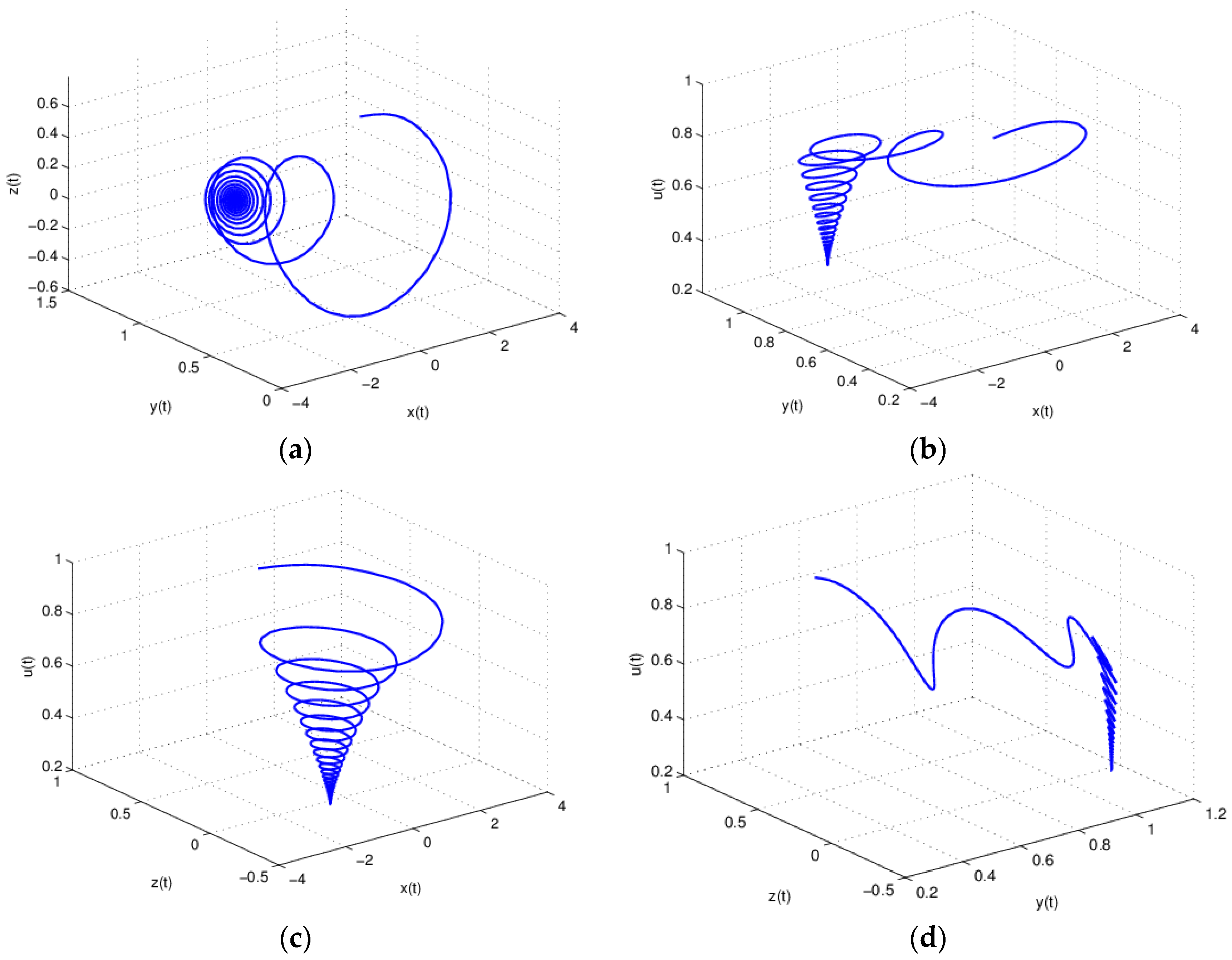
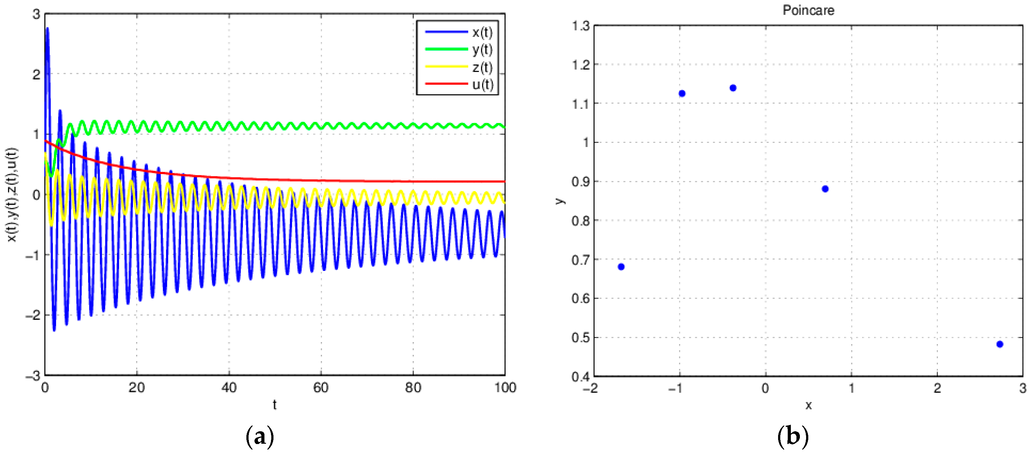
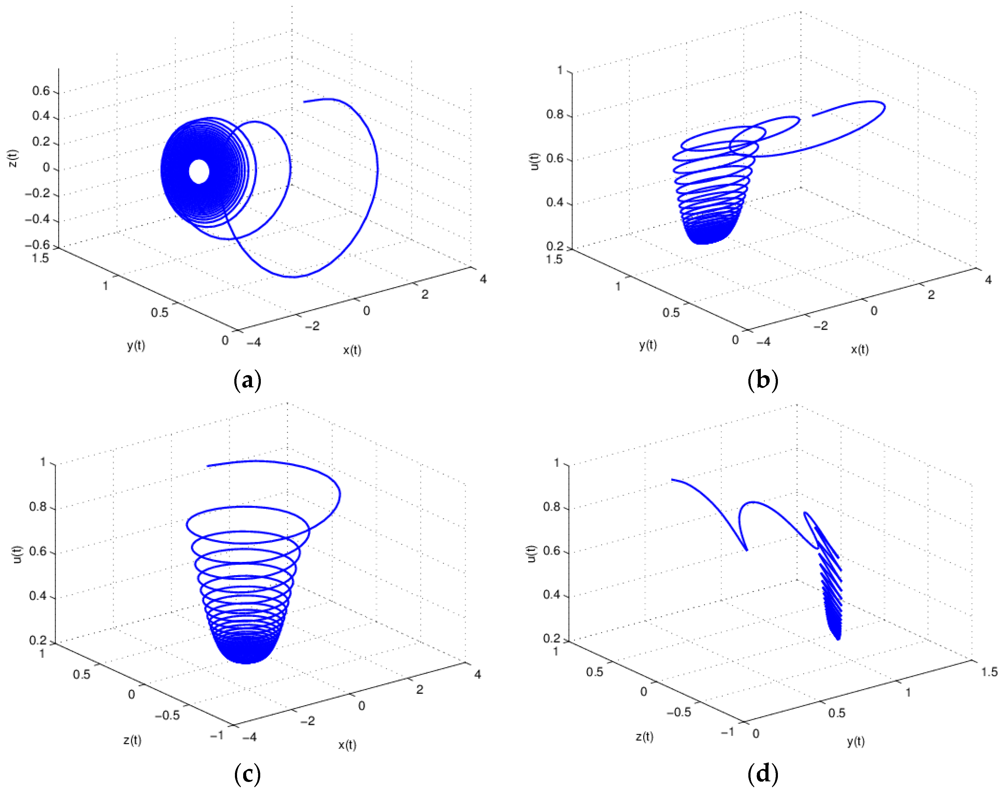
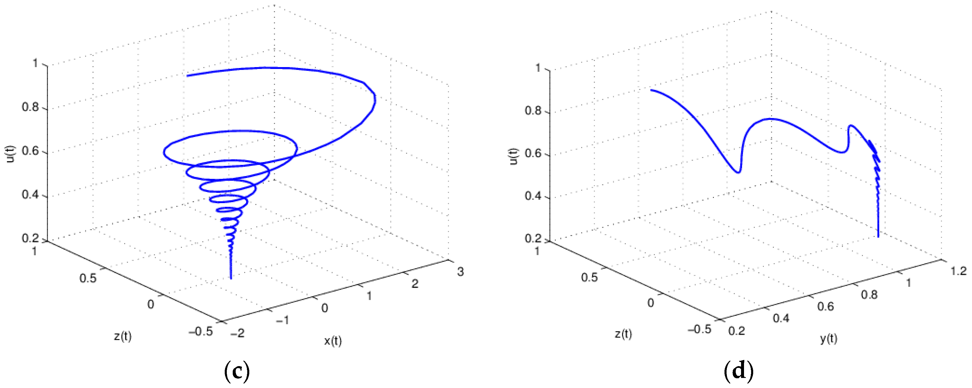
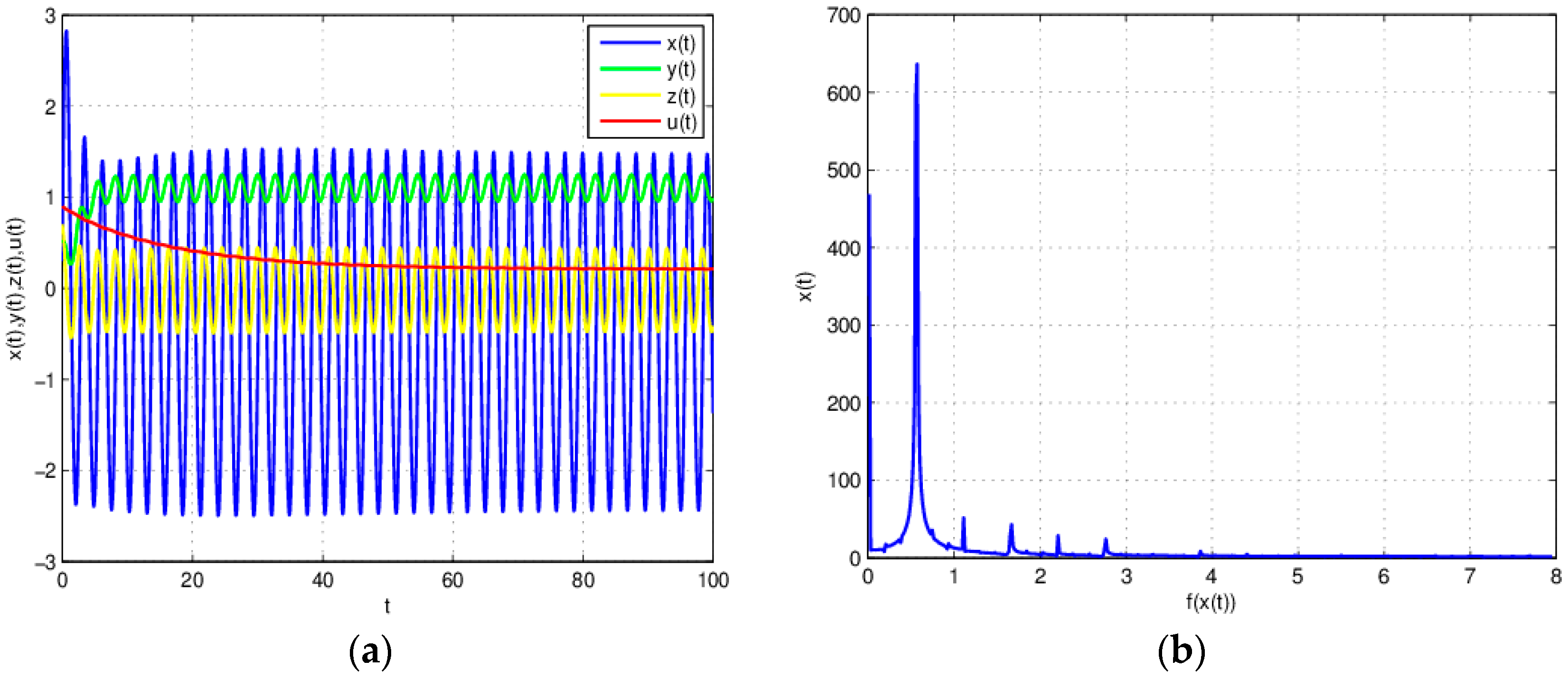
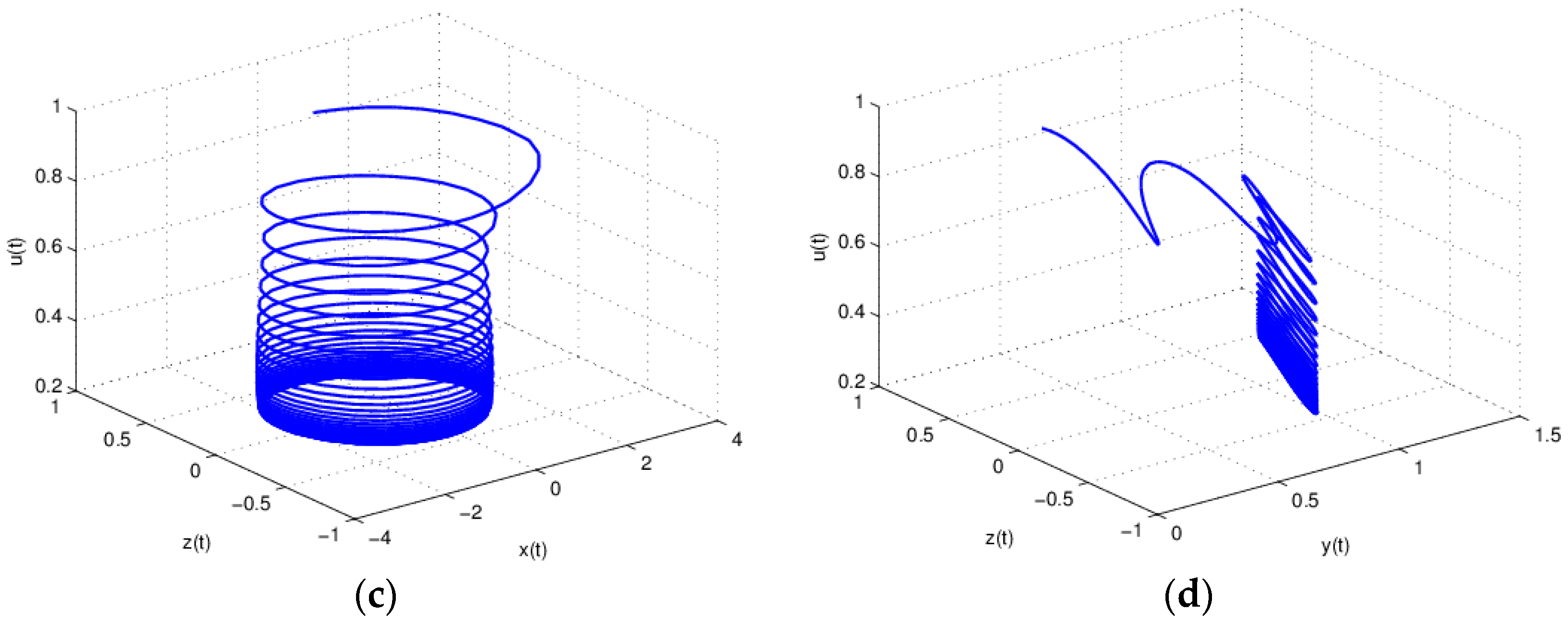
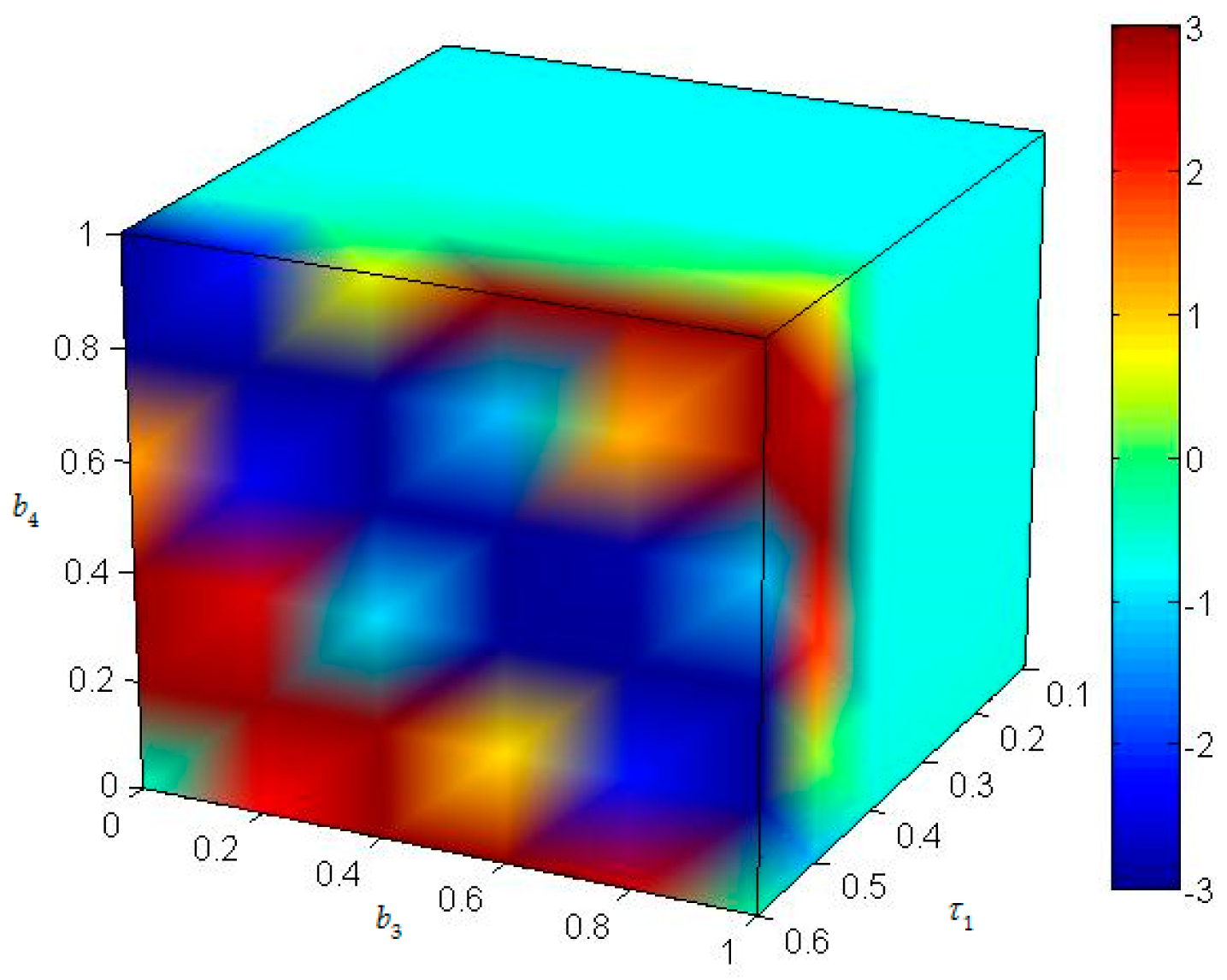
3. Numerical Simulation and Analysis
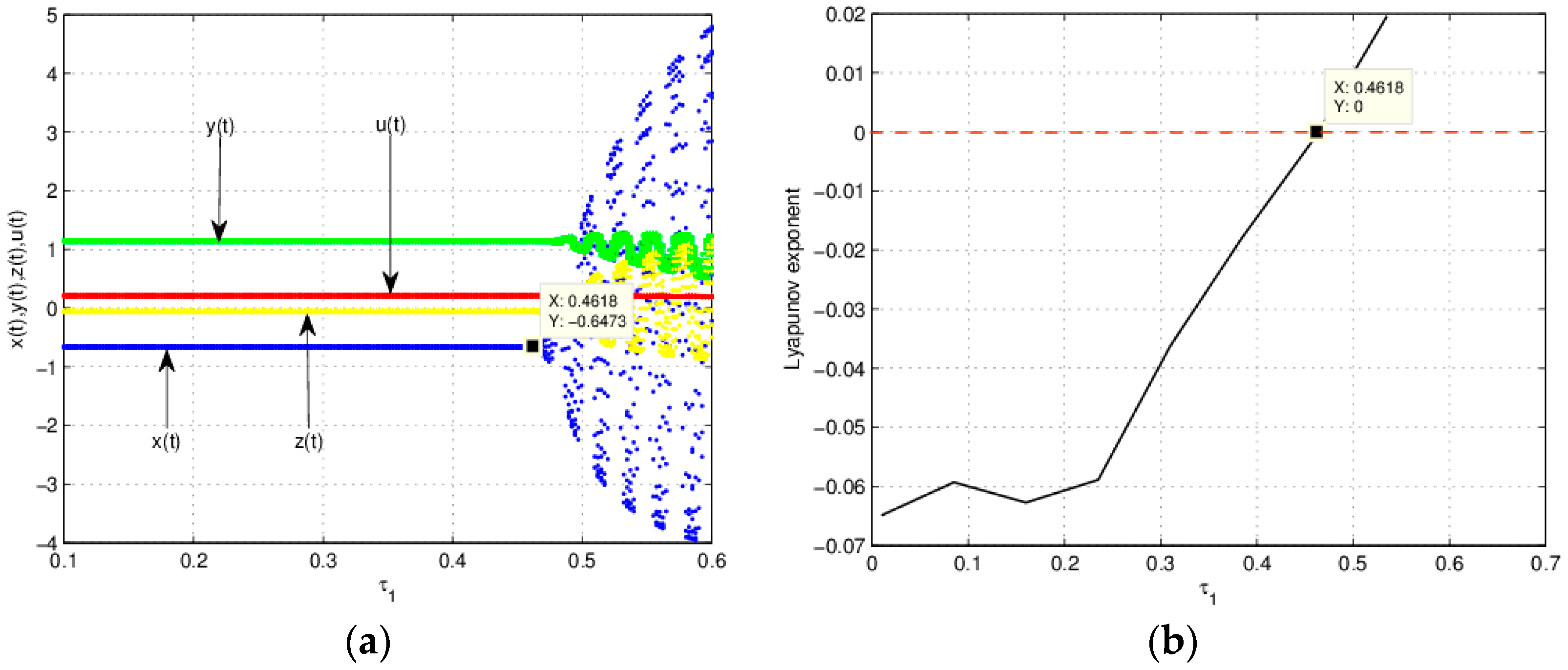
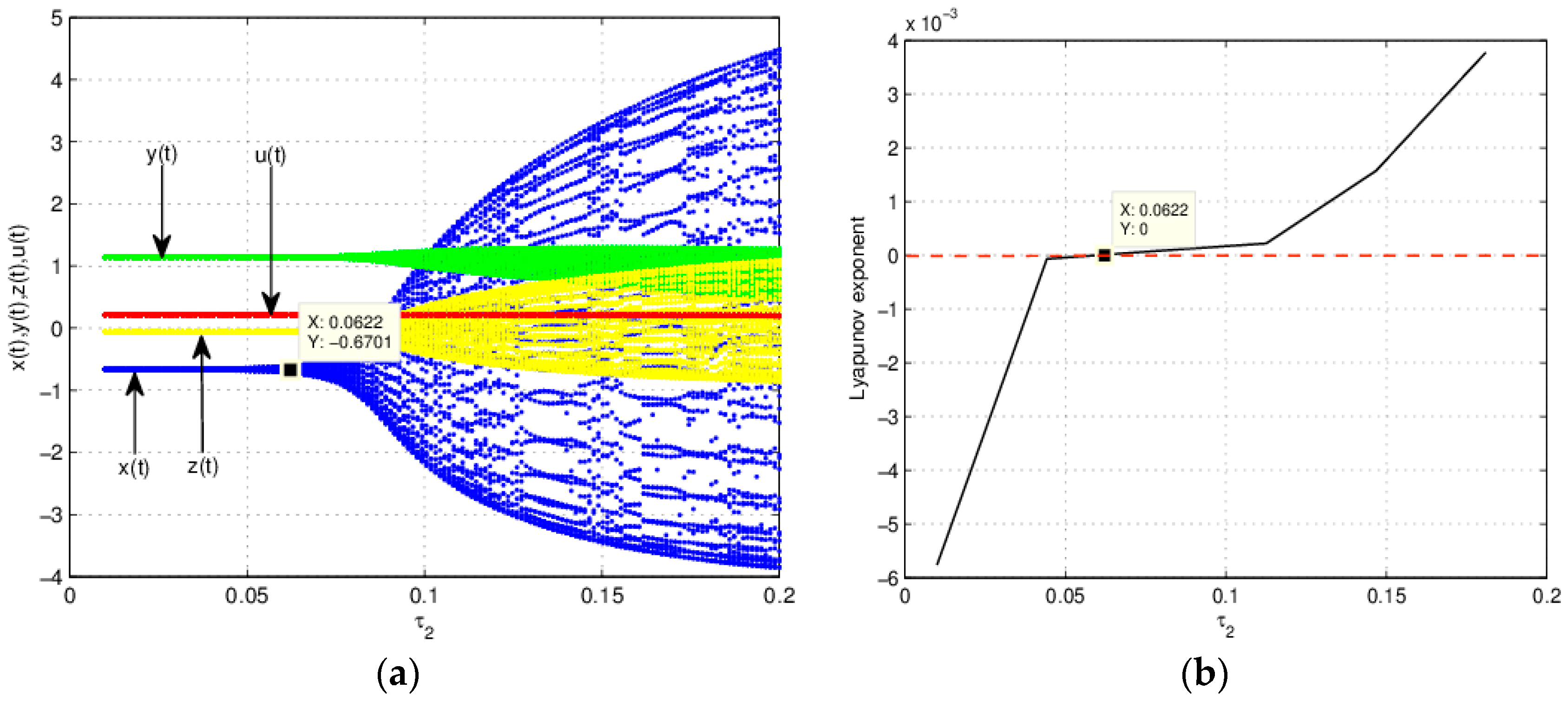
3.1. The Influence of on the Stability of Equation (19)
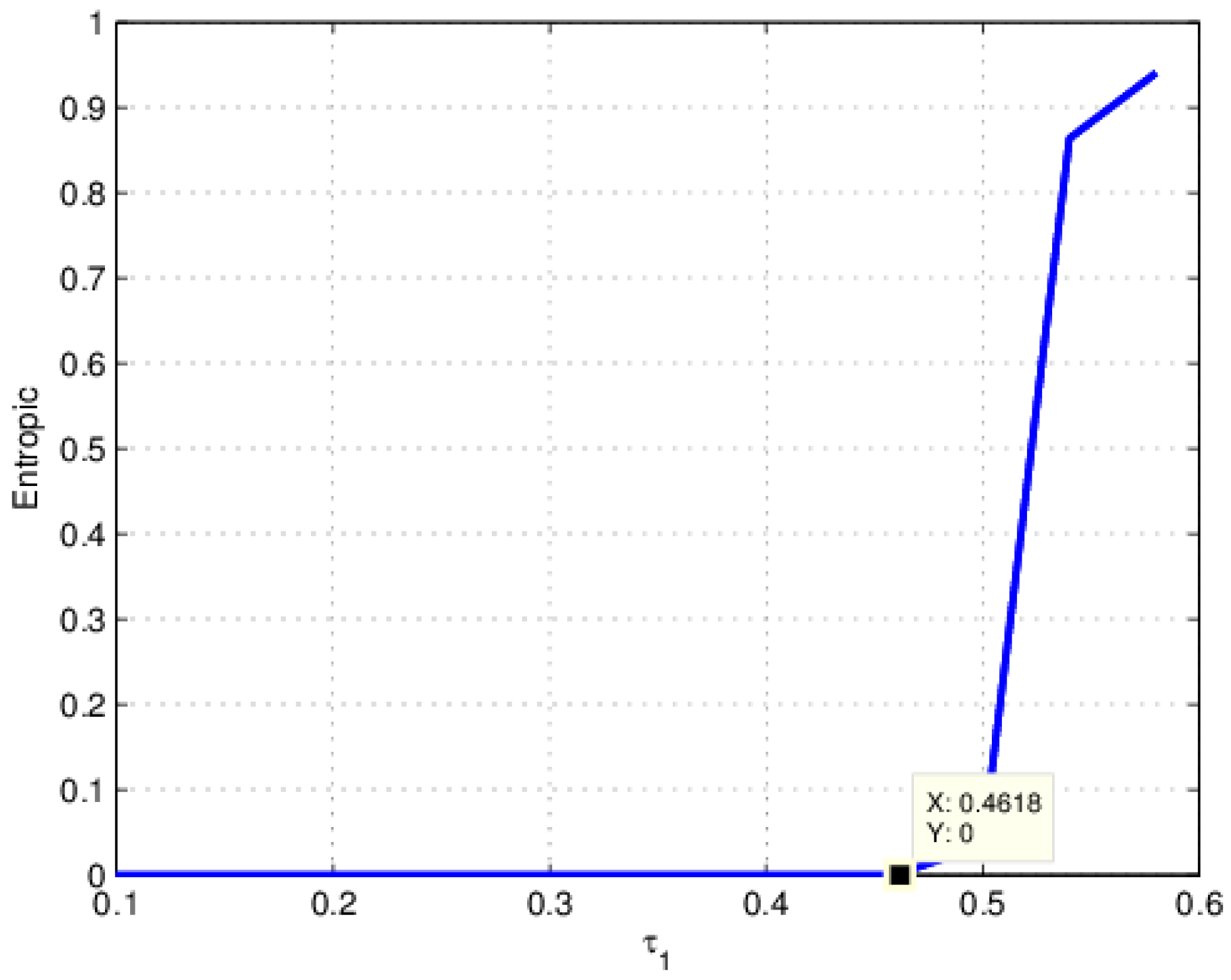
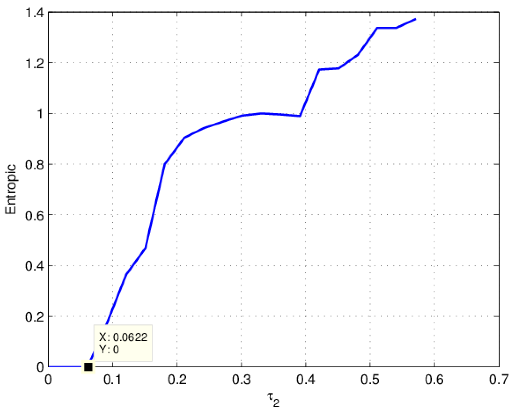
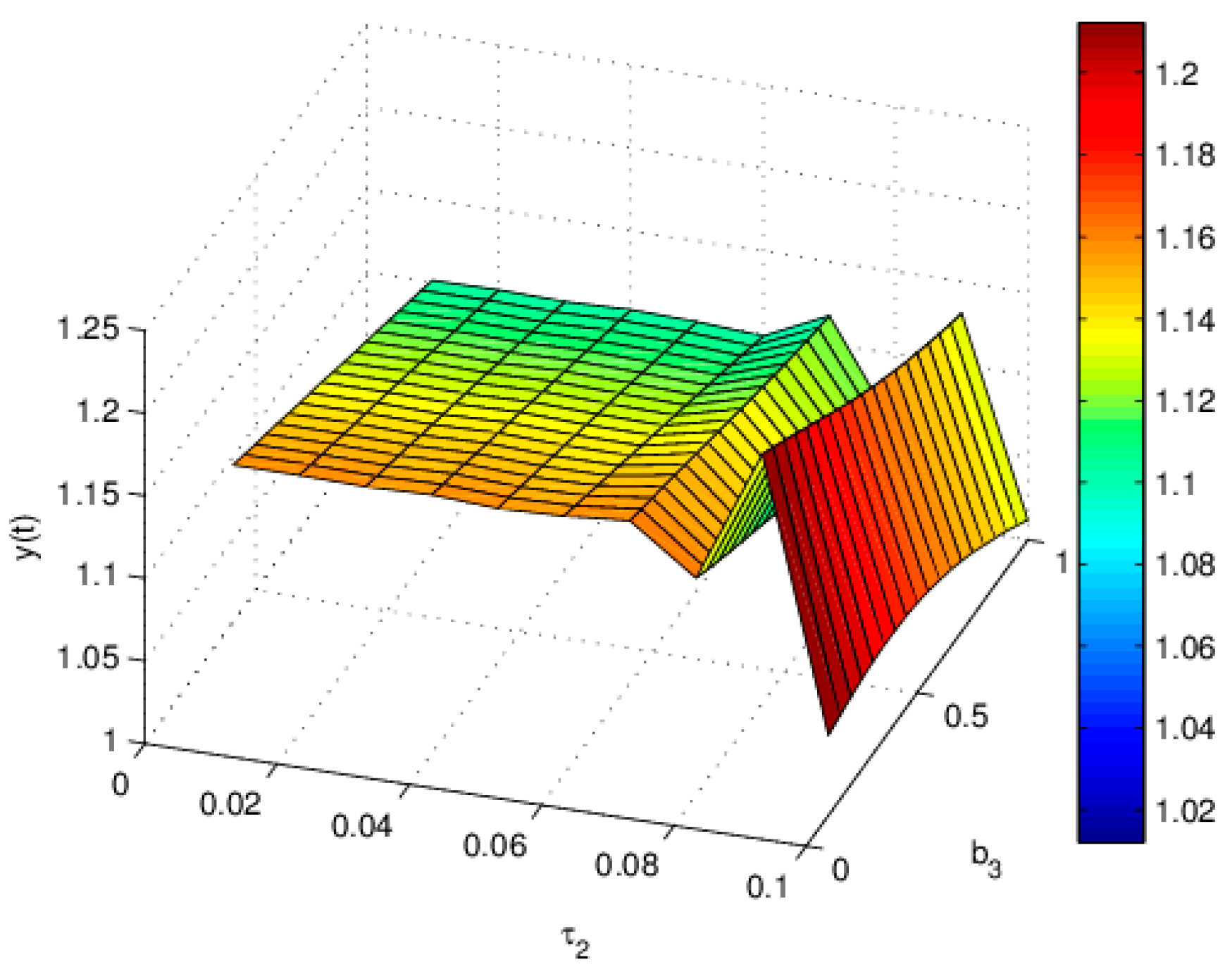
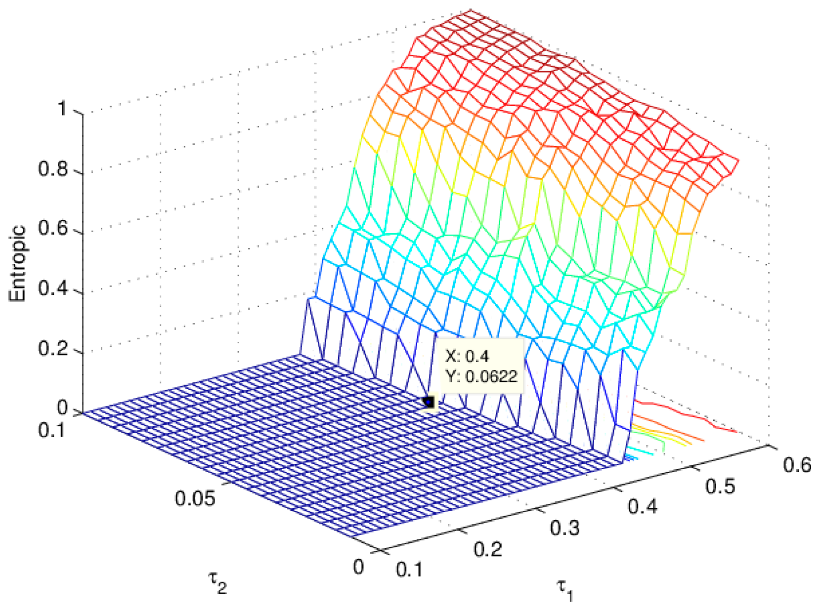
3.2. The Influence of on the Entropy of Equation (19)
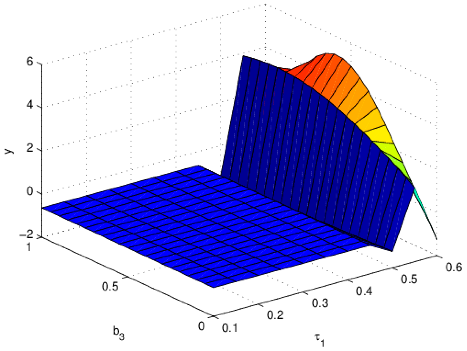
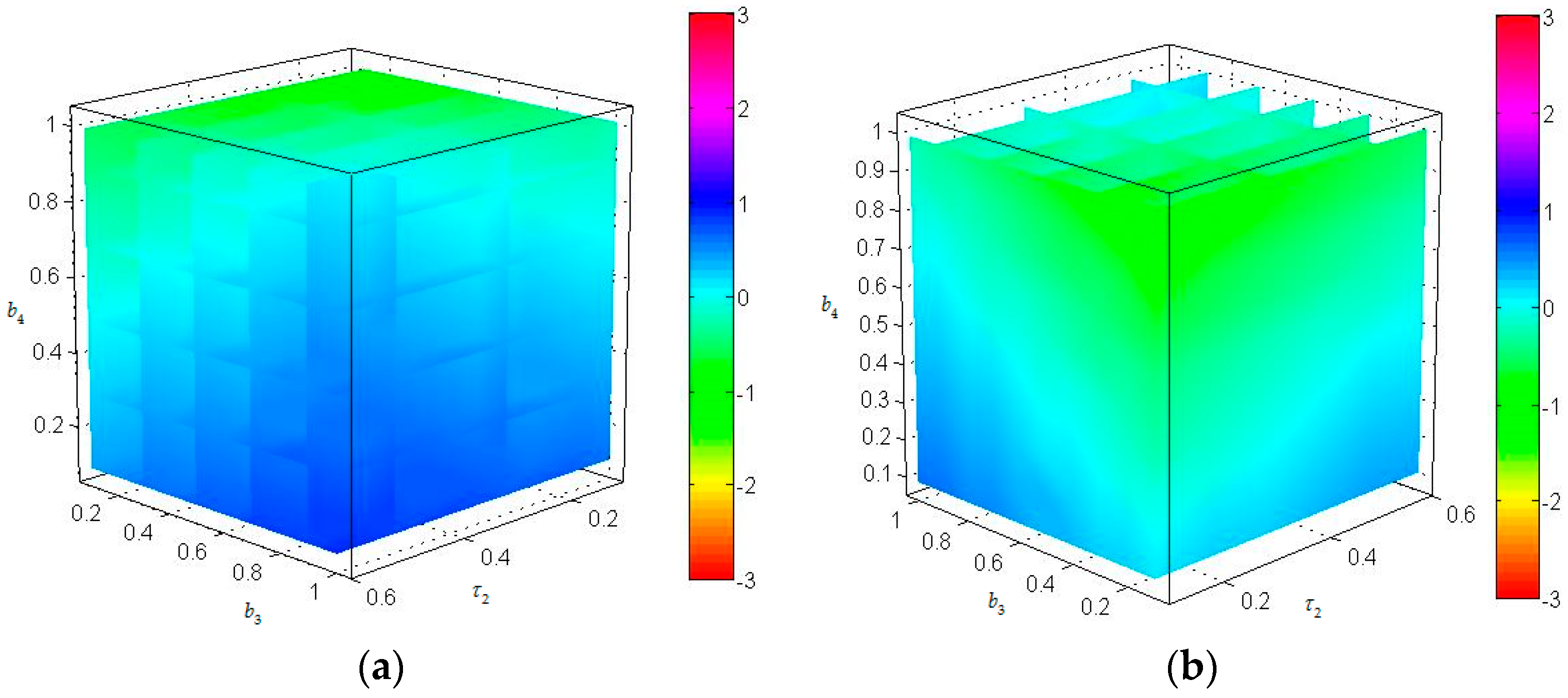
3.3. The Influence of on the Stability of Equation (19)
3.4. The Influence of on the Stability of Equation (19)
3.5. The Influence of on the Entropy of Equation (19)
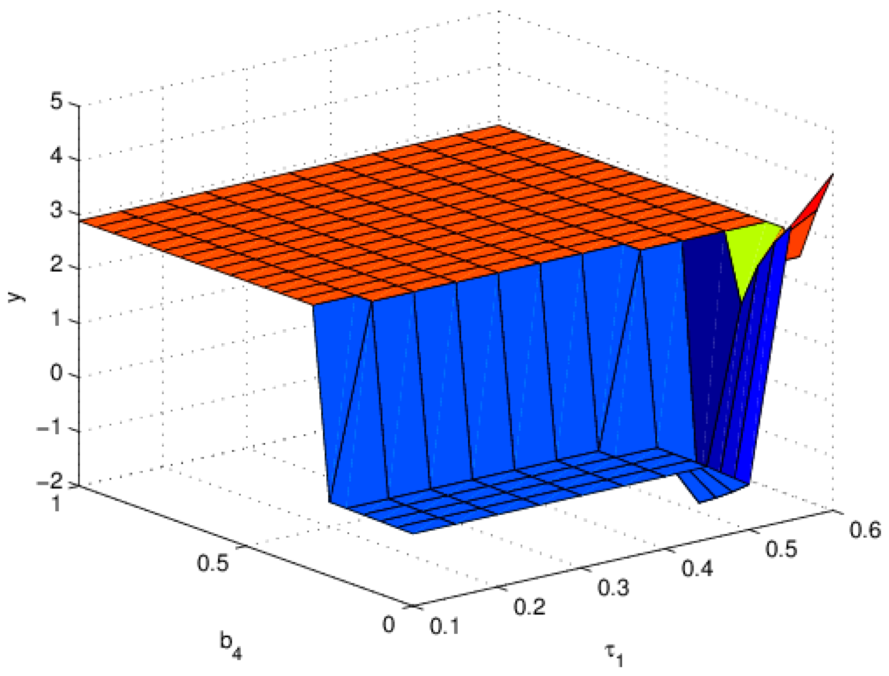
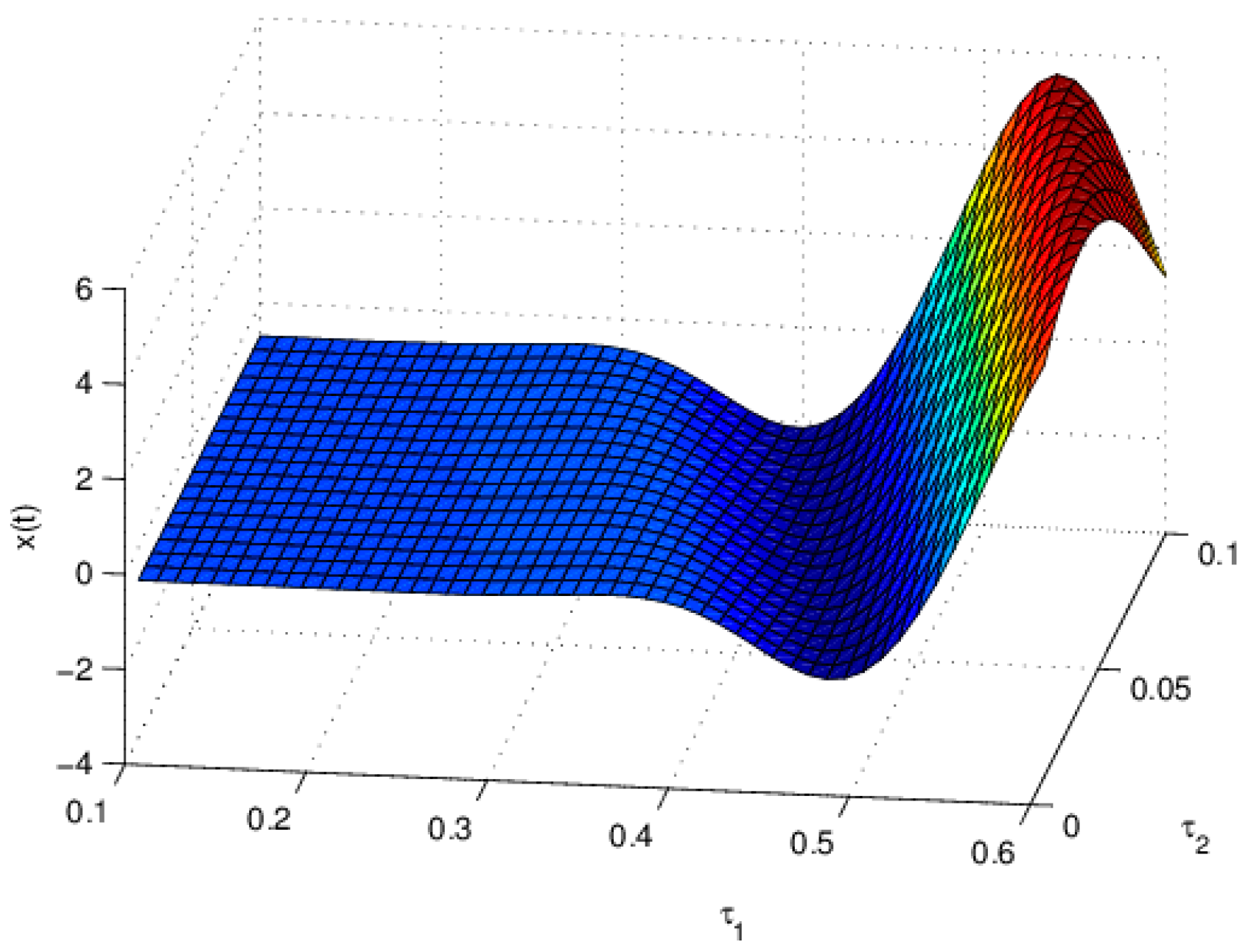
3.6. The Influence of on the Stability of Equation (19)
3.7. The Influence of on the Stability of Equation (19)
3.8. The Influence of on the Entropy of Equation (19)
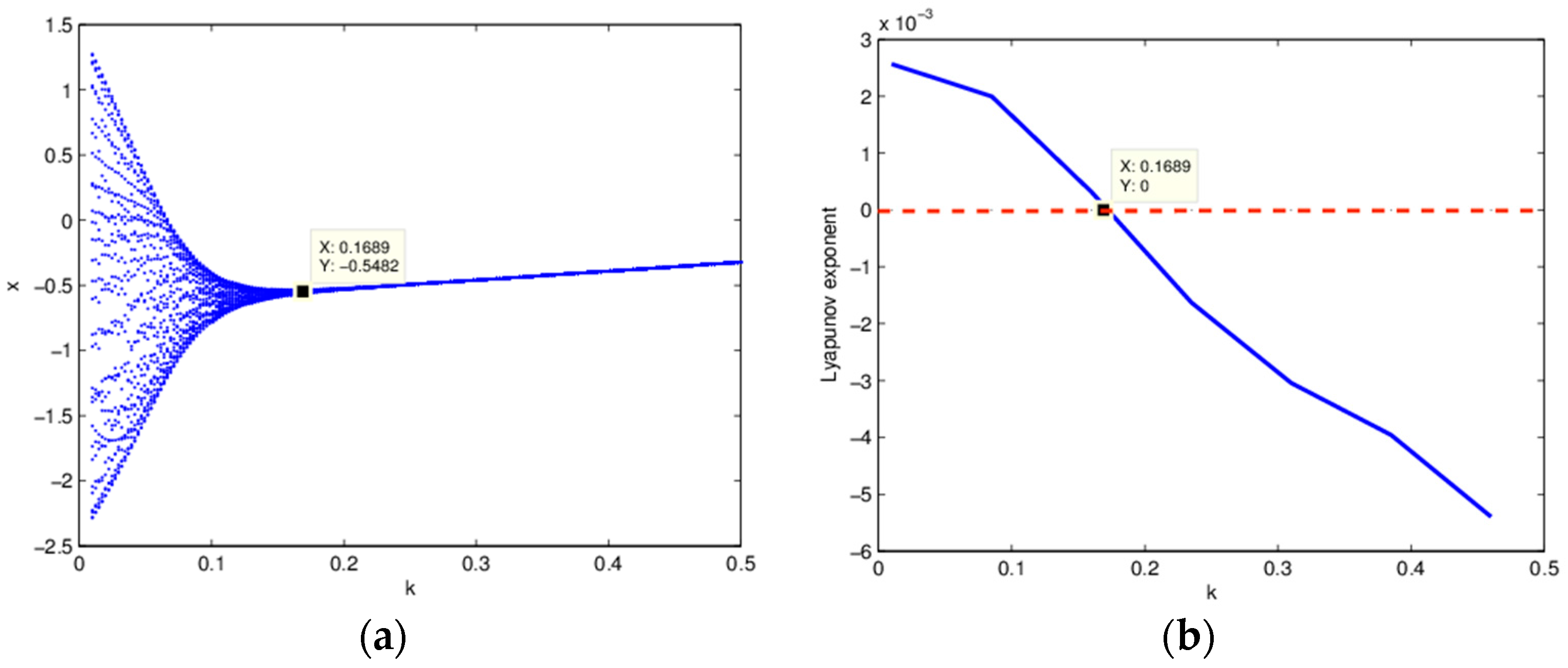
4. Bifurcation Control
4.1. Bifurcation Value of Equation (20) to
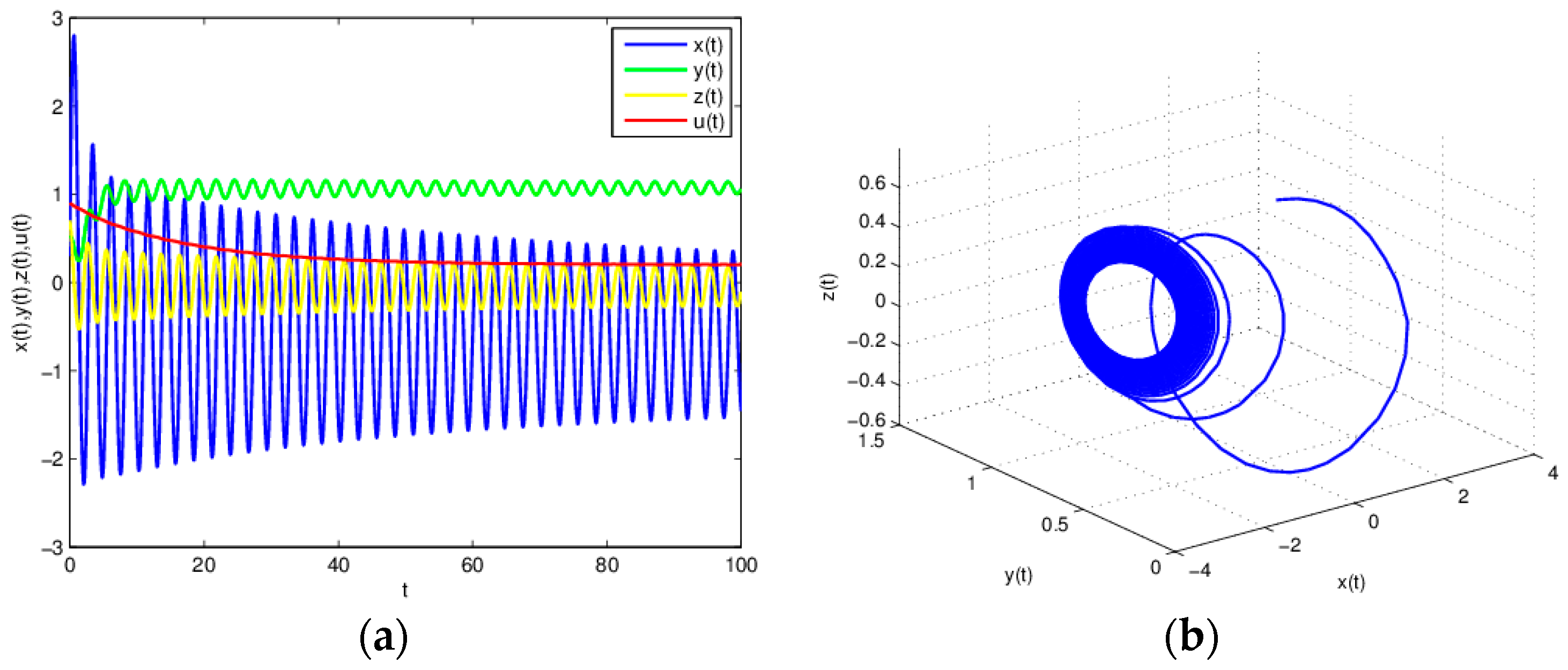
4.2. Equation (20) is Unstable When
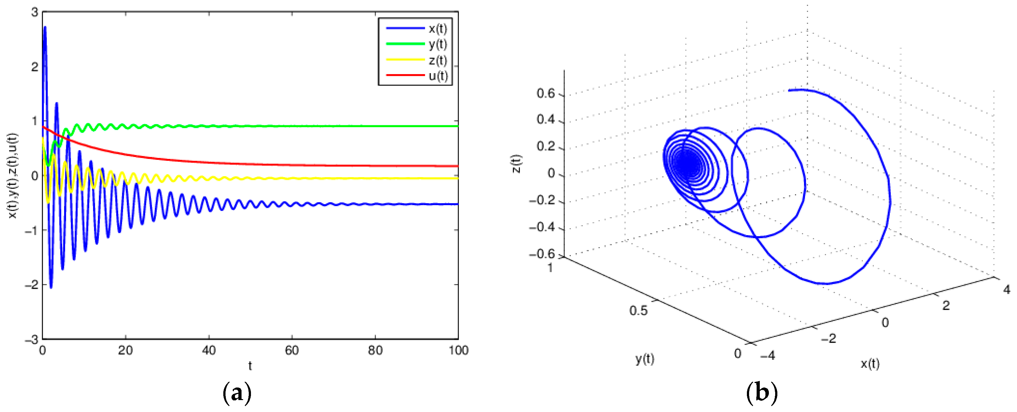
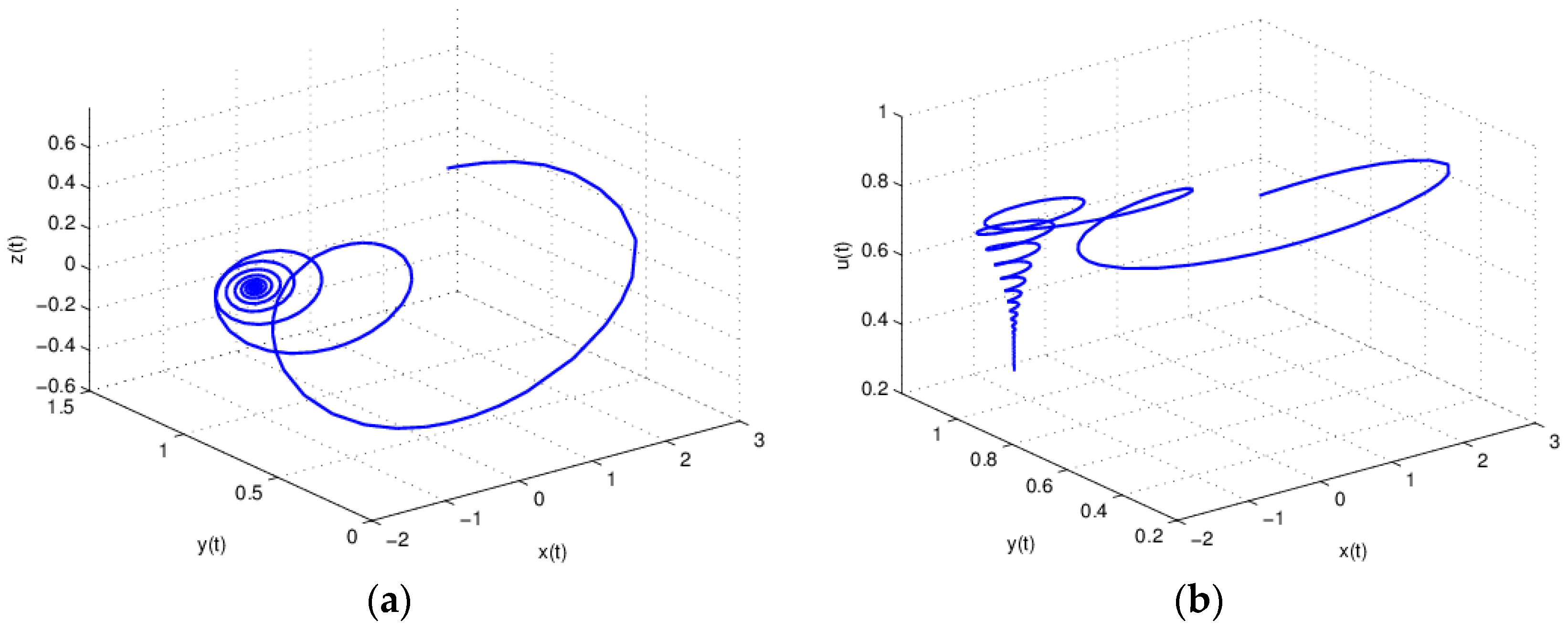
4.3. Equation (20) is Stable When
5. Conclusions
Acknowledgments
Author Contributions
Conflicts of Interest
References
- Lv, T.; Zhou, L. Dynamics of energy price model with time delay. J. Quant. Econ. 2012, 4, 15–19. [Google Scholar]
- Tian, L.; Zhao, L.; Sun, M. Energy resources structural system for Jiangsu Province and its dynamical analysis. J. Jiangsu Univ. 2008, 1, 82–85. [Google Scholar]
- Strachan, N.; Kannan, R. Hybrid modeling of long-term carbon reduction scenarios for the UK. Energy Econ. 2008, 6, 2947–2963. [Google Scholar] [CrossRef]
- Gerlagh, R. A climate-change policy induced shift from innovations in carbon-energy production to carbon-energy savings. Energy Econ. 2008, 2, 425–448. [Google Scholar] [CrossRef]
- Zhang, Y. Supply-side structural effect on carbon emissions in China. Energy Econ. 2010, 1, 186–193. [Google Scholar] [CrossRef]
- Fang, G.; Tian, L.; Sun, M.; Fu, M. Analysis and application of a novel three-dimensional energy-saving and emission-reduction dynamic evolution system. Energy 2012, 40, 291–299. [Google Scholar] [CrossRef]
- Lorenz, E.N. Deterministic no periodic flow. J. Atmos. Sci. 1963, 2, 130–141. [Google Scholar] [CrossRef]
- Chen, G.; Ueta, T. Yet another chaotic attractor. Int. J. Bifurc. Chaos Appl. Sci. Eng. 1999, 7, 1465–1466. [Google Scholar] [CrossRef]
- Lü, J.; Chen, G. A new chaotic attractor coined. Int. J. Bifurc. Chaos Appl. Sci. Eng. 2002, 3, 659–661. [Google Scholar] [CrossRef]
- Sun, M.; Tian, L.; Fu, Y.; Qian, W. Dynamics and adaptive synchronization of the energy resource system. Chaos Solitons Fractals 2007, 4, 879–888. [Google Scholar] [CrossRef]
- Sun, M.; Tian, L.; Zeng, C. The energy resources system with parametric perturbations and its hyper chaos control. Nonlinear Anal. Real World Appl. 2009, 4, 2620–2626. [Google Scholar] [CrossRef]
- Sun, M.; Wang, X.; Chen, Y.; Tian, L. Energy resources demand-supply system analysis and empirical research based on non-linear approach. Energy 2011, 9, 5460–5465. [Google Scholar] [CrossRef]
- Liu, X.L. Probing the guiding role of taxation in energy-saving and emission-reducing Technology. Energy Procedia 2011, 5, 20–24. [Google Scholar]
- Gao, C.W.; Li, Y. Evolution of China’s power dispatch principle and the new energy saving power dispatch policy. Energy Policy 2010, 38, 7346–7357. [Google Scholar]
- Wang, M.; Xu, H. A Novel Four-Dimensional Energy-Saving and Emission-Reduction System and Its Linear Feedback Control. J. Appl. Math. 2012, 2012, 1–14. [Google Scholar] [CrossRef]
- Song, Y.; Wei, J. Bifurcation analysis for Chen’s system with delayed feedback and its application to control of chaos. Chaos Solitons Fractals 2004, 22, 75–91. [Google Scholar] [CrossRef]
- Kuznetsov, Y.A. Elements of Applied Bifurcation Theory; Springer: New York, NY, USA, 2004. [Google Scholar]
- Gori, L.; Guerrini, L.; Sodini, M. Hopf bifurcation and stability crossing curves in a cobweb model with heterogeneous producers and time delays. Nonlinear Anal. Hybrid Syst. 2015, 18, 117–133. [Google Scholar] [CrossRef]
- Ma, J.; Guo, Z. The parameter basin and complex of dynamic game with estimation and two-stage consideration. Appl. Math. Comput. 2014, 248, 131–142. [Google Scholar] [CrossRef]
- Galias, Z. Basins of Attraction for Periodic Solutions of Discredited Sliding Mode Control Systems. In Proceedings of the 2010 IEEE International Symposium on Circuits and Systems, Paris, France, 30 May–2 June 2010; pp. 693–696.
- Du, J.; Huang, T.; Sheng, Z. Analysis of decision-making in economic chaos control. Nonlinear Anal. Real World Appl. 2009, 10, 2493–2501. [Google Scholar] [CrossRef]
- Matsumoto, A. Controlling the Cournot-Nash chaos. J. Optim. Theory Appl. 2006, 128, 379–392. [Google Scholar] [CrossRef]
- Agiza, H.N. On the Analysis of stability, Bifurcations, Chaos and Chaos Control of Kopel Map. Chaos Solitons Fractals 1999, 10, 1909–1916. [Google Scholar] [CrossRef]
- Holyst, J.; Urbanowicz, K. Chaos control in economic model by time-delayed feedback method. Phys. A Stat. Mech. Appl. 2000, 287, 587–598. [Google Scholar] [CrossRef]
- Guo, Y.; Xu, D. Synchronizing Chaos by Variable Feedback Control. J. Northwest. Polytech. Univ. 2000, 5, 277–280. (In Chinese) [Google Scholar]


© 2016 by the authors; licensee MDPI, Basel, Switzerland. This article is an open access article distributed under the terms and conditions of the Creative Commons Attribution (CC-BY) license (http://creativecommons.org/licenses/by/4.0/).
Share and Cite
Wang, J.; Wang, Y. Study on the Stability and Entropy Complexity of an Energy-Saving and Emission-Reduction Model with Two Delays. Entropy 2016, 18, 371. https://doi.org/10.3390/e18100371
Wang J, Wang Y. Study on the Stability and Entropy Complexity of an Energy-Saving and Emission-Reduction Model with Two Delays. Entropy. 2016; 18(10):371. https://doi.org/10.3390/e18100371
Chicago/Turabian StyleWang, Jing, and Yuling Wang. 2016. "Study on the Stability and Entropy Complexity of an Energy-Saving and Emission-Reduction Model with Two Delays" Entropy 18, no. 10: 371. https://doi.org/10.3390/e18100371