1. Introduction
A common analysis when dealing with -omics data sets of thousands of variables is to
rank all these variables according to some measure that identifies how important they are to predict and/or retrospectively understand a certain disease characteristic or outcome. An example of a scenario is to study gene expression data of cancer patients and a class variable that identifies whether the patient relapsed or not. In this case, such analysis can be used as a first step of variable selection for the later application of other sophisticated statistical and/or biological experiments, as it may avoid expensive time-consuming analyses using uninteresting variables, or at least may help to prioritize them and save valuable resources [
1]. Quor is a method designed to compare independent samples with respect to corresponding quantiles of their populations and to provide a confidence value for the order of such arbitrary quantiles. This confidence on the order of the quantiles can be used to build a ranking of importance for the variables in a domain. As an example, suppose we have two populations (healthy and ill subjects) and are interested in the median values of a variable representing the level of expression of a particular gene. The goal is to obtain the confidence that “the median expression of that gene in the first population is strictly smaller (respectively greater) than the median expression of the same gene in the second population”. The comparison of medians might suggest that the gene is under- or over-expressed in the ill subjects, or simply that there is no significant difference of expression between the populations. By applying such computation to all genes in a data set, one can rank them based on the obtained confidence values.
Often, approaches for ranking variables may rely on unrealistic assumptions, such as normality of samples, asymptotic behavior of statistics, approximate computations, comparisons of only two populations/groups, need of equivalent number of samples in the groups (across distinct variables, not simply across groups), among others [
2]. For instance, methods for hypothesis testing such as the Student’s
t-test and the Mann–Whitney–Wilcoxon’s rank–sum
u-test [
3,
4,
5] have been widely employed for such purposes. Their statistics (or their
p-values) are often used to sort variables into some ranking of importance. Arguably, they represent the most commonly used methods for this problem in biomedical applications (even if they were not originally devised for such purpose). Quor is nonparametric and assumes nothing but independence of samples, which may potentially increase its applicability and is particularly useful when assumptions of other methods cannot be asserted. It can deal with different numbers of samples and missing data, and yet can properly compare these variables. Its computations are very efficient using a simple dynamic programming idea and are performed using exact distributions with no need for any asymptotic consideration. Other ideas to work with quantiles do exist. For instance, [
6] developed confidence intervals for different quantiles of a single population, while Quor targets two or more populations and only one quantile (abeit not necessarily the same) in each population.
Experiments with simulated data suggest that Quor might be a better option when the underlying assumptions of other methods are suspected not to hold. In particular, Quor achieves greater area under the receiver operating characteristic (ROC) curves than many competitors, such as t-test, u-test, Mood’s median test, and others. We also employ multiple real benchmark -omics data sets to empirically compare Quor and other methods with respect to the ranking of the variables they provide. It is shown that the rankings produced by Quor have better relation to the accuracy of group prediction based on a univariate model (with the variable in question). Finally, a study with copy number data of diffuse large B-cell lymphoma patients demonstrates the use of Quor with quantiles other than the median and indicates that Quor may produce better ranking than other methods (including the standard method for that problem, that is, the Fisher exact test applied after the categorization of the variables).
2. Methods
We describe here the details of Quor and present an efficient algorithm for its computation. The method is built on the ideas of confidence statements developed long ago [
7,
8] and revisited more recently [
9]. The proposed method uses nonparametric confidence intervals for quantiles based on the binomial distribution [
10]. Its goal is to compute a confidence value indicating how much one believes that quantile parameters of different populations/groups are ordered among themselves. This confidence can be loosely related to standard confidence regions used in frequentist analysis, as we explain later on. We do not assume any particular quantile nor a specific number of populations, even though the case of comparing medians of two populations is arguably the most common scenario for its application. For ease of expose, we will present the method using two groups, but the extension to three or more groups is straightforward.
The problem is defined as follows. Let
and
represent, respectively, the quantiles at arbitrary percentages
and
for two populations, that is,
with
(these inequalities are tight in the continuous case). Let
be a sorted sample of size
from population
. The goal is to compute a confidence value in
that indicates how much we believe in the statement
(or similarly
). This value can and will be used later to rank variables in an order of the confidence that the underlying populations have such difference in their quantiles.
Let
be the sorted vector of
independent and identically distributed random variables from population
j (random variables from distinct populations are not necessarily identically distributed). Since the probability of one observation being smaller than the population quantile
is
, it is straightforward that it holds for
(that is, the
ith
order statistics):
and
These inequalities come from probabilities obtained with a binomial distribution with
trials and probability of success
(they are inequalities because of possible ties at
in the discrete case only). Consider a pair of order statistics
and the event
. Given the independence assumptions, one can compute
using the product of binomial probabilities from Equations (
2) and (
3) (in the discrete case, a lower bound for the probability is obtained).
The samples
and
are assumed to be sorted non-decreasingly (one could easily sort them beforehand if they were not). After these samples are observed, the only unknown quantities of interest are the quantiles
and
of the two populations being studied. By replacing random variables with their observations, we create the statement
as follows:
which has confidence given by Equation (
4). Note that the statement e is only a function of the order statistics
and
and not of the actual observed values of
and
, and these order statistics are only what is needed in order to compute using Equation (
4) (assuming that the data are available at hand). At this point after sampling, the value of Equation (
4) becomes a confidence value instead of a probability [
7]. This confidence regards the unknown quantities of interest, in our case the parameters
and
. If we take each part of the statement e in Equation (
5) separately (namely,
and
), then the corresponding values obtained for these statements, computed through Equations (
2) and (
3), are actual confidence values in the frequentist statistics jargon. Because of the independence assumption between the samples, we take their product as the confidence of the statement e itself.
Now, the idea is to look for statements
that are able to tell us something about the order between
and
. With a quick inspection of Equation (
5), we have
that is, the assertion in the left-hand side of Equation (
6) implies an order for the quantiles, thus its confidence is a lower bound for the confidence of the right-hand side. Because we know how to compute the confidence value of
through Equation (
4), and because any time the assertion
is false the Equation (
6) is not applicable, we run over all pairs
of orders such that
and keep the maximum confidence value of the e statements built from these pairs as our estimation for the confidence that
holds true:
Hence, we use the left-hand side of Equation (
7) as our confidence about
. We can take the maximum value because each confidence value
is an actual confidence for
; thus, it is possible to use the one yielding the greatest confidence. The value, however, might only be an approximation to
because of the gap between
and
. Since we want to obtain a maximal value, a mathematical property that speeds up computations is to choose
such that
is the smallest possible value greater than
, that is, the value of
, in order to maximize the confidence, is uniquely and easily computable from the value
(this holds because there is no reason to leave a larger gap between
and
if a smaller gap is possible, as smaller gaps will certainly yield higher confidence values). Hence, we only need to optimize over the possible values of
to find the highest confidence value. Such a procedure is presented in Algorithm 1. We recall that if one wants to compute the confidence of
, then they simply need to rename the variables accordingly before invoking the algorithm, while if one wants to check for every possible order of the quantiles (for instance, when we are not interested in a particular order a priori), then both permutations are to be checked.
| Algorithm 1 (Quor Core) Confidence value of a statement about the ordering of quantile parameters of two populations. |
Input a data set with samples , for , and the quantiles of interest and
Output the confidence value that the statement holds true.
- 1
Pre-compute the values that appear in Equations ( 2) and ( 3) by making a cache. For : and for :
- 2
|
Theorem 1. Algorithm 1 uses space and time , with .
Proof. Step 1 pre-computes the partial binomial sums. By doing it in a proper order, this can be accomplished in constant time for each , and the loop will execute times. Step 2 performs a very simple dynamic programming, with steps in the outer loop. The inner argmin can be accomplished with an overall total of steps by keeping a pointer to the last found of each outer loop (because the vectors are sorted, the next result of argmin cannot be smaller than that, and so only one pass over each possible is done). Hence, Step 2 takes time in the worst case too. ☐
Algorithm 1 is very fast (as fast as hypothesis testing methods such as the Wilcoxon rank–sum test). The correctness of Algorithm 1 comes from its simple dynamic programming formulation. At each loop of Step 2, we find a pair yielding the highest possible confidence value for that given , and the loop iterates over all possible . It is worth noting that some computations in Algorithm 1 could suffer from numerical problems. We have addressed this issue by implementing it using incomplete beta functions and/or arbitrary precision in particular cases where n is quite large (many hundreds). Because of caching, this does not slow down the whole approach in a perceivable way.
The confidence value obtained with Quor provides information about differences in quantiles as well as similarities in quantiles (for example, in the case that confidence is low in both directions). This is in contrast to usual hypothesis testing, where no evidence in favor of the null hypothesis can be obtained. Finally, we point out that the ideas presented here can be extended to any number of groups. Derivations and algorithm implementation become more intricate, but overall computational complexity is still low. In order to give a sketch of the version with any number of groups, the dynamic programming needs to keep track of the order statistics of each of the groups in Step 2, which needs to further iterate over the m groups, achieving worst case time complexity bounded by m times the complexity for two groups. The complexity does not considerably increase (becomes only quadratic in m) because the dynamic programming keeps track of all optimal candidates for previously processed groups (there are at most m of them). We omit such more sophisticated versions for ease of exposition, and for the fact that working with two groups is, by far, the most common and interesting case, as we discuss in the sequel.
3. Results
The experiments are divided in simulated and real data studies with multiple -omics data sets. We use the first part of this section to discuss the benefits of Quor in terms of prediction accuracy with simulated data. Then, we use multiple data sets to show the quality of the produced ranking of Quor and widely used methods.
3.1. Simulation Study
We compare Quor to a number of competitors, namely (i) the two-sample
t-test, which performs an analysis of means by comparing their normalized difference to a
t distribution; (ii) the Mann–Whitney–Wilcoxon
u-test, which checks whether the probability of an observation from one distribution being greater than an observation from another is equal to
; (iii) the modified
t-test as presented in the package
samr [
11]; (iv) the standard Mood’s median test; and (v) the
q-test for quantile testing [
12]. Ranking covariates by the statistics of such tests is reasonable as long as the number of data samples is constant over all covariates (in which case the ranking can be equivalently done by sorting
p-values). Each test has a different assumption about the distributions under null/alternative hypotheses. We choose as target quantiles for Quor the medians (so we are interested in ordering the medians of the populations) unless stated otherwise.
The goal of these experiments is to understand the goodness of the confidence value of Quor to identify the difference in the populations. We will draw a parallel to the p-values obtained by t- and u-tests. It is obvious that these procedures should only be used in cases where their assumptions hold. However, verifying whether their assumptions hold is by itself subject to issues. Bear in mind that we will perform analyses without trying to check if their assumptions are satisfied, and, in fact, we will analyze their behavior exactly in those cases where they are not.
To make results comparable, we study the area under the receiver operating characteristic (ROC) curve, as it is a measure (independent of any chosen threshold) for the prediction accuracy of the methods in identifying whether a gene is differently distributed in the two given groups. As argued recently by many statisticians [
13], this approach for comparison of methods does not force the use of a particular significance level without justification. In the case of Quor, a high confidence value (above a certain threshold) would conclude that there is a difference (in that gene) between populations, while for
t- and
u-tests, a small value of the
p-value (below a certain threshold) is used to achieve such a conclusion. The experiments consist of generating samples either from the same distribution for the two groups (in this case, we hope that the methods will not identify any difference) and from two different distributions (in which case, the methods should identify the difference). The ROC curve is built by varying the threshold value that each method uses to decide whether the samples are from the same or different distributions. In order to generate different distributions for the groups, we use the following two scenarios: an experimental setting with a mixture of Gaussians (a common assumption in biomedical analyses, including gene expression) and another with Gaussians. The amount of difference between the generating distributions of the two groups will be quantified by a single parameter
θ, as explained in the continuation.
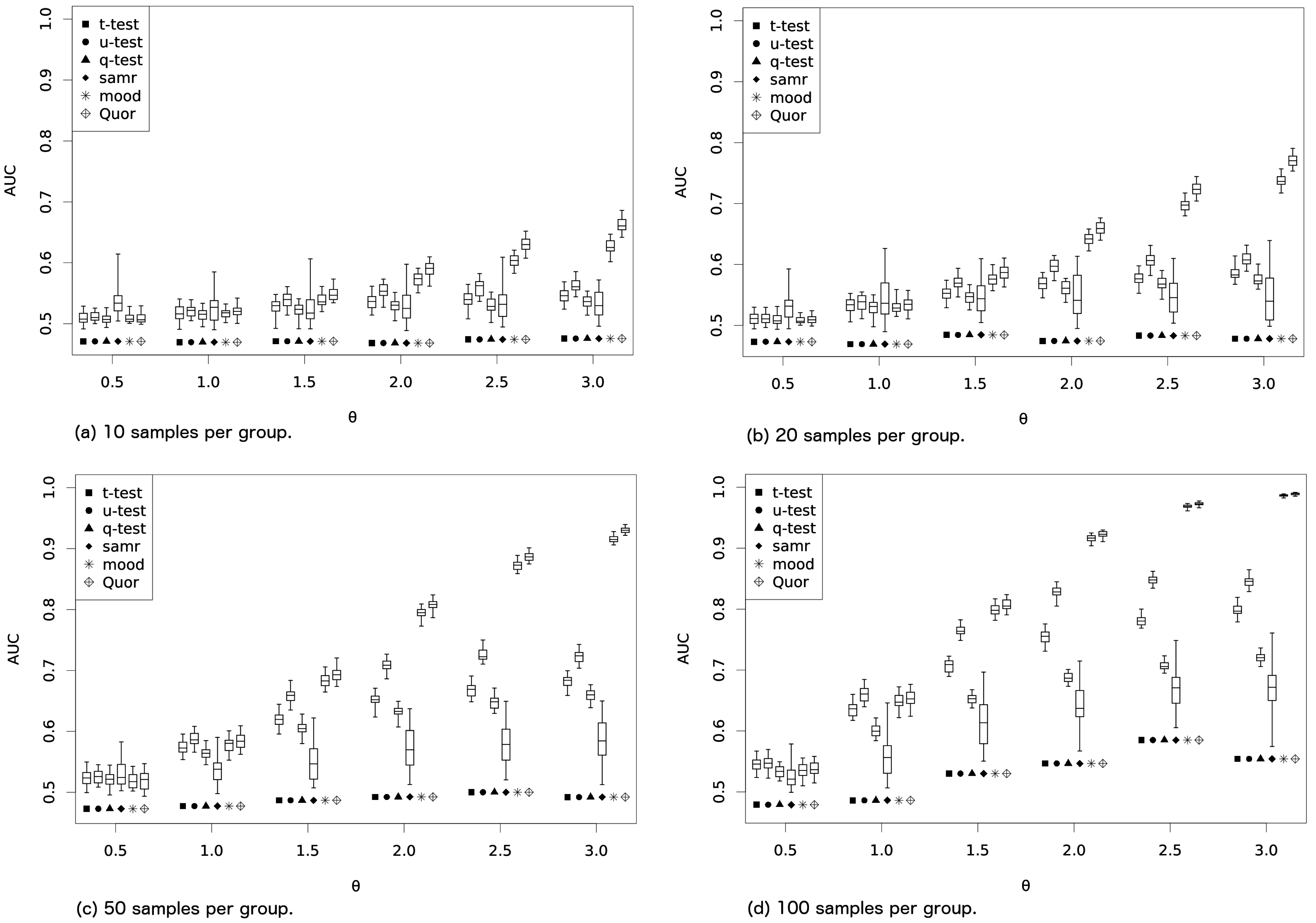
As a first experiment, all methods are run to identify the (nonexistent) difference between samples generated from a Gaussian with mean zero and standard deviation two (for each of the two groups). This is repeated 100 times with 2000 simulated genes each time (1000 in each group), and the results from the methods are recorded. The two groups are sampled as follows: (i) the first group from a mixture of two Gaussians with means equal to and (both Gaussian standard deviations ) and with weights 2/3 and 1/3 for the mixture, respectively; and (ii) the second group from a mixture of two Gaussians with weights 1/3 and 2/3 for Gaussians with means and (standard deviations again equal to two). All methods are run over the 2000 genes and results are recorded. Each of these 2000 points indicates whether a method successfully identified if the curves were the same (first thousand points) or different (next thousand points), so we have the amount of true/false positives and true/false negatives. Now, the area under the ROC curve is calculated using these 2000 values for each method. The high number of evaluations gives us a very precise picture of the area under the curve for each of the methods. This procedure is repeated 100 times and boxplots are constructed.
Our choice of mixture distributions is designed to produce faster variation in the medians than in the means when one increases the single experimental parameter
θ. Hence, with the increase of the
θ, the first group will have its mean and median decreasing, while the second will experience its mean stalled and its median increasing. Results are shown in
Figure 1 over the variation of the
θ from 0.5 to 3 that is used to define the generating distributions (for each value of
θ, the area under the ROC curve is computed using 2000 points and repeated 100 times). The experiment is conducted for sample sizes (same for the two groups) in
. From the figure, it is clear that Quor produces better results (larger area under the curve) than the other methods because the difference in the medians with the increase in
θ grows faster than the difference in the means (so this is nothing but expected). Moreover, Quor does better than
u-test (which should account better for the difference in medians than the
t-test),
q-test and Mood’s median test, which are designed to check differences in medians.
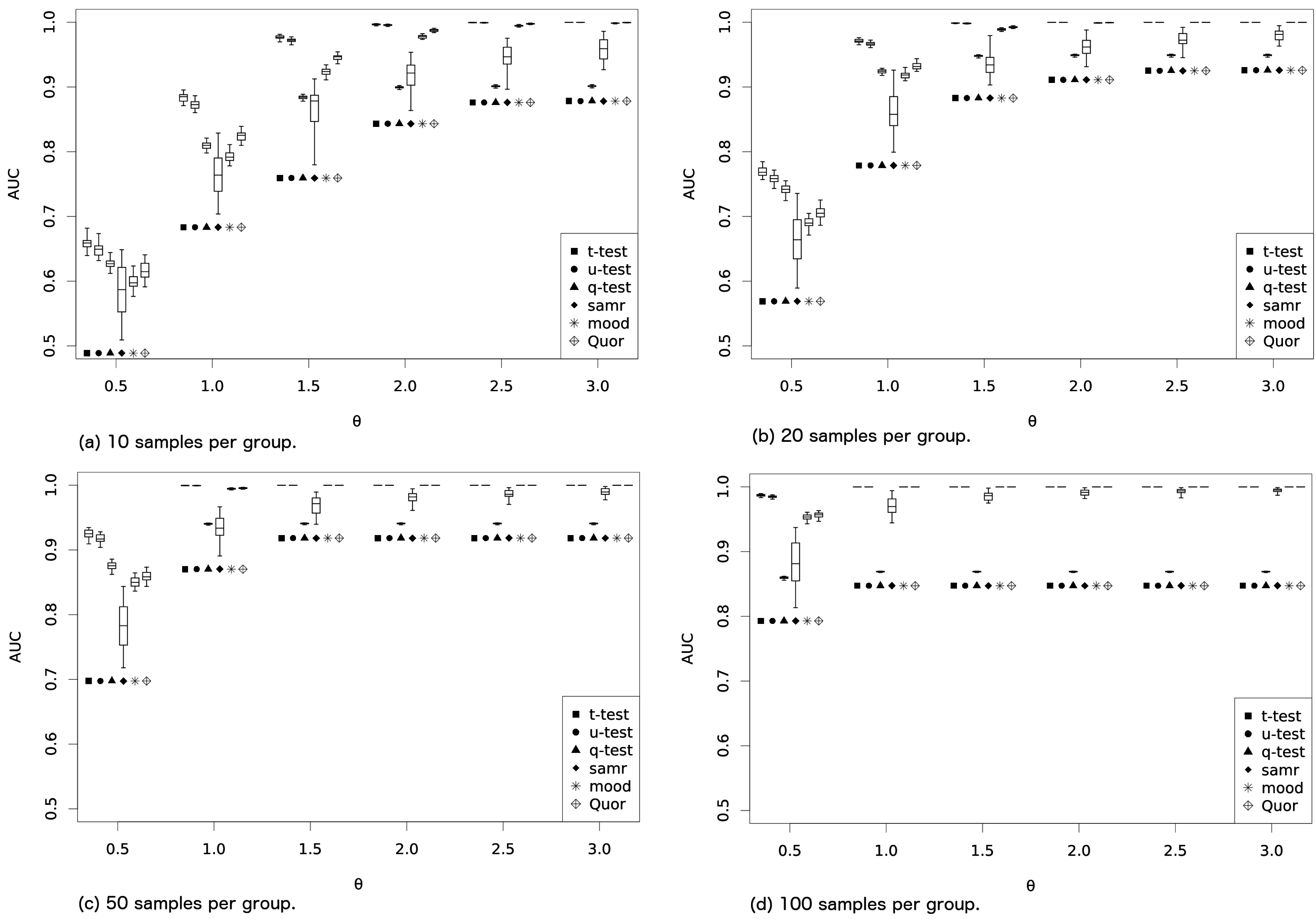
While in the first batch of experiments we have used mixtures of Gaussian with medians that varied faster than means (thus benefiting Quor and the other quantile methods), in the second batch, we perform experiments with Gaussians so as to see whether
t-test considerably dominates the other methods (as in this case its assumptions are fulfilled and the
t-test is expected to perform better). Again, methods are run to identify the (nonexistent) difference between samples generated from a Gaussian with mean zero and standard deviation two (100 repetitions with 1000 genes each). We generate the groups from (i) a Gaussian with mean
; and (ii) a Gaussian with mean
(standard deviations always as
). One hundred repetitions are run once more with 2000 genes each, so again we have 1000 cases where no difference between groups should be identified and 1000 cases where a difference should be identified by the methods. Results of the area under the curve are displayed in
Figure 2. In this case, and as expected,
t-test and
u-test perform better, with
t-test slightly superior, although the difference is not so prominent. We argue that if one does not know whether the data are Gaussian, Quor might be a better choice. It produced better results when data were from a mixture of Gaussians, while not losing too much accuracy in the Gaussian experiment. Even though it produced worse results in this latter case, Quor directly returns which group has the greater quantile without any additional effort, which might be an extra benefit.
3.2. Comparison and Discussion on Rank Evaluation in -Omics Data Sets
The analysis of -omics data deals with several thousands (or millions) of variables, which, for instance, may represent the expression of genes or the copy number of genomic regions. When the study is performed genome-wide, it is a common procedure during the analysis to somehow sort the variables with respect to their “performance”, in order to select which of them should be considered in further investigations/experiments. This is especially important in recent data where the number of variables has become extremely large and sophisticated analyses over all variables would require prohibitive computational resources.
In this section, we apply the same methods as before except for the q-test (namely t-test, u-test, modified t-test from samr, Mood’s median test and Quor) to the task of ranking the variables in some order of importance/preference using multiple -omics data sets. The q-test has been discarded from this and forthcoming experiments because of its poor quality in the simulated data and its terrible computational performance. The rank of the variables is defined for each method in the following way. When using t-, u- or Mood’s median tests, we sort the variables by their p-values (in increasing order, as generally done in the literature), for the modified t-test of samr we use its absolute score, while, for Quor, we sort them by the confidence values (decreasingly).
We consider two main applications. Firstly, we compare the quality of the obtained ranks by using eight benchmark data sets of gene expression profiling and proteomic spectra. In this situation, the rank of each variable is assessed on the basis of its capability in group classification [
1]. Secondly, we apply the appropriate methods to a copy number data set of diffuse large B-cell lymphoma (DLBCL) patients, and we compare the ranks (yielded by different approaches) for well-established aberrations characterizing the three cell-of-origin subtypes.
3.2.1. Performance in Group Prediction
We compare the obtained ranking from the different methods on a collection of benchmark data sets.
Table 1 presents the data sets used for this comparison. The data were obtained from internet repositories, and we defer further details to their corresponding citations (see
Table 1).
For the purpose of evaluating the quality of the obtained ranking (yielded by each method), we would need to know the correct rank of the variables, which is unavailable in real data and cannot even be easily simulated (as the true ranking for a data set is a characteristic of the available samples and not of an underlying distribution). To overcome this drawback, we follow a previous study [
1] and employ as our target the ranking obtained by sorting variables according to their accuracy when used alone for group prediction, that is, for each variable we compute the zero-one loss (prediction error) of a simple classification model that predicts which is the group of each individual using only that single variable. This is done using the whole data set and forms the ranking to which we will compare all other methods. We use the
R package
rpart, but any similar idea would suffice, as the information available to build the model leads to splitting the image of the predictive variable into pieces—we allow at most two splits to avoid an obvious overfit. We call this ranking the target ranking.
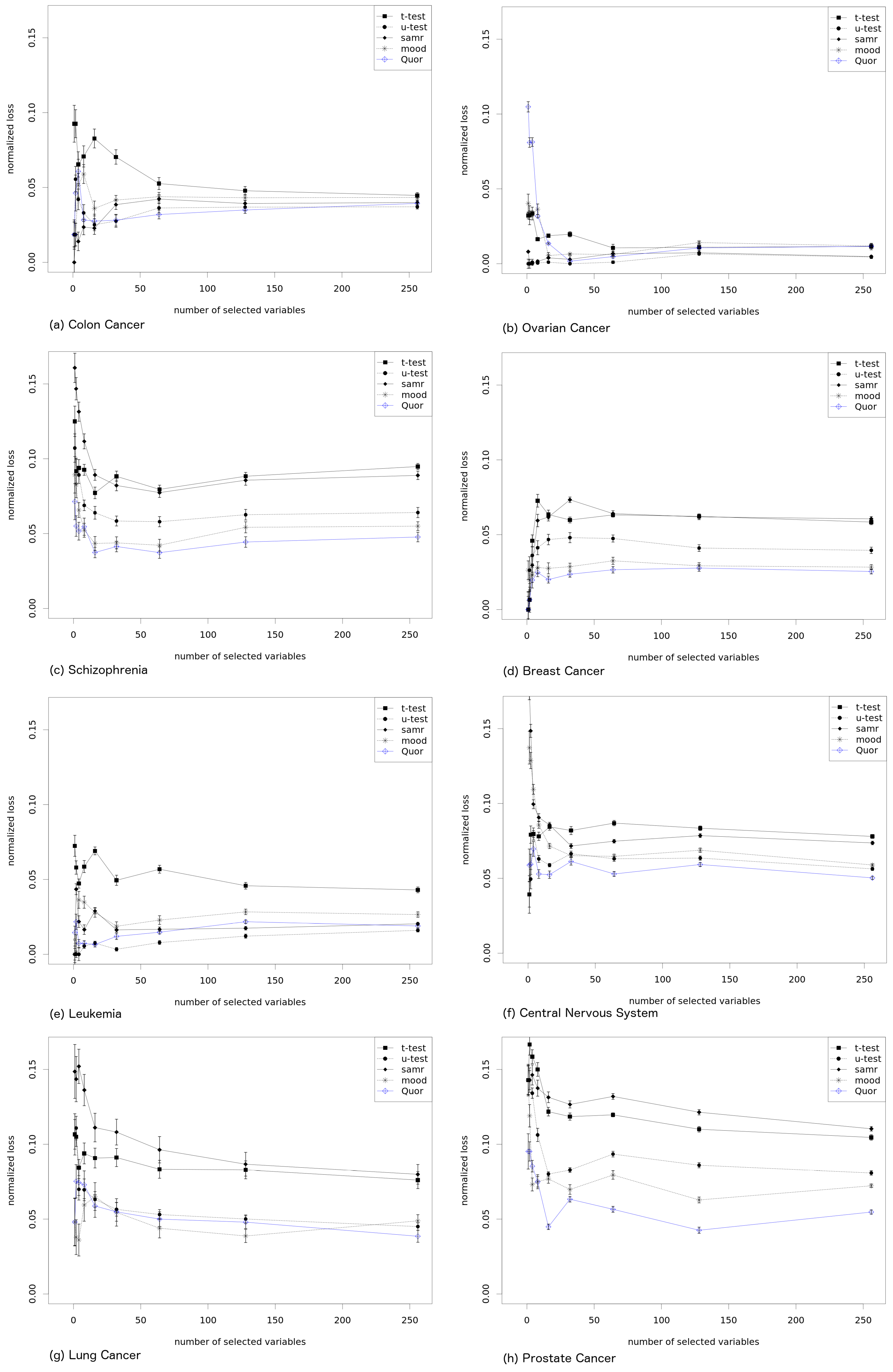
We evaluate each method by taking the
k best ranked variables according to it (for arbitrary different values
k, as shown in the horizontal axis of
Figure 3) and by computing the average prediction accuracy that such
k best variables have according to the target ranking. A better method will result in lower values, since the prediction accuracy of the variables that are within the
k best variables will reflect how the obtained ranking identifies the important variables which are exactly those with small rank value in the target ranking). For clarity of presentation, we divide such averaged accuracy value by that obtained by the target ranking, which is obviously optimal in this respect. The results in
Figure 3 (for the data sets described in
Table 1) show how far (in percentage) the named method is from the target rank. A value of zero in the curve means that the ranking was as good as the target rank, and higher values indicate worse performance, as the subset of variables has larger (averaged) prediction error (the correct ranking is assumed to have the optimal order in terms of prediction error). Each point in the graph is obtained by subsampling half of the data available for each gene and group. This is repeated 20 times, and the graph shows mean values and standard deviations (as bars). Hence, the methods have access only to part of the data, while the computation of the target ranking has been done with the whole data set.
Quor has different characteristics from the other methods, in particular from the
t-test. Results in
Figure 3 show an overall worse performance of the
t-test (as well as of its modified version from
samr), which has produced ranks with less prediction accuracy in almost every data set and almost every number of selected variables (suggesting that the produced rank is not very related to group prediction accuracy). Quor, Mood’s median and
u-test achieved better results, with Quor showing a clear superiority in three or four data sets and
u-test in only one. Mood’s median test show good results but is consistently outperformed by Quor.
3.2.2. Identifying Well-Known Lesions in Copy Number Data
As a second application, we analyze the copy number (CN) microarray data of the 176 DLBCL patients of [
22], for which the classification in the three following cell-of-origin subtypes was available: 71 germinal center B-cell like, or GCB; 74 activated B-cell like, or ABC; and 31 primary mediastinal B-cell lymphoma, or PMBL. DNA copy number aberrations are defined as genomic regions with a number of copies of DNA different from two (which is the normal value for autosomal chromosomes). Thus, the CN profile of a patient can be represented as a piecewise constant function, where segments showing an increased CN are called gains, while the ones with a decreased CN are called losses. The microarray CN data contain continuous values, due to both technical and biological reasons, and after applying a segmentation method, the regions of gains and losses are usually detected by using some thresholding (defined opportunely). As for this study, the data of [
22] were obtained segmented and both with and without discretization in gains/losses/normal CN, from the Progenetix database [
23]. Quor,
t-test and
u-test are applied to the continuous segmented data (with the goal of demonstrating the differences with respect to Quor), while the Fisher exact test (that can be referred as a standard method for the analysis of CN data) to the already discretized data. Mood’s median test is not used as it has been consistently outperformed by Quor.
Heterogeneous diseases, like DLBCL, are characterized by aberrations that might be present only in 15%–35% of the cases, and disease subtypes may share some lesions [
22,
24]. Therefore, when testing a possible aberration related to DLBCL subtypes, we consider each possible test of two subtypes versus the remaining one, in order to find whether the aberration is prominently associated with any single one of the groups. Moreover, due to the low frequency of lesions in these data [
22,
24], Quor can be used in an opportune way by comparing quantiles of the distributions other than the median. For example, a gain may be identified associated with a group when the 85th quantile of its distribution is higher than the 95th quantile of the distribution of the other group (so we use
and
and compute the confidence of
), while a loss may be identified when the 15th quantile of a group is lower than the 5th quantile of another (in this case, we use
and
). Hence, Quor has been configured to identify differences in the tails of the distributions, which shows its ability to test different characteristics according to one’s needs. We also include in the analysis the method Quor with median as target quantile for comparison. The Fisher exact test is performed as usual by testing a single type of aberration at a time (gain versus not gain and loss versus not loss). In the analysis, we consider all the genomic regions with at least five probes, obtained by the union of all segmented profiles. For each region and for each method, all evaluations are performed, and the best result is chosen to define the
p-value or the confident value used in the ranking (multiple test correction is unnecessary, as orders are preserved).
Notice that in this setting the variables (i.e., the genomic regions) are highly dependent (for example, the first 20 regions identified by Quor when comparing the tail-related quantiles are all at cytobands 9p24 and 9p21). Nevertheless, the five approaches for ranking the regions are compared with respect to the yielding rank achieved in well-established CN lesions (shown in
Table 2) associated with DLBCL cell-of-origin subtypes. The results are showed in
Table 3, where ranks for each of those well-known lesions were identified. This study regards a common situation in the analysis of this type of data: regions are sorted according to some measure of importance and further analyses are performed with those regions which appear first (with low rank). With that in mind, Quor, using the tail-related quantiles, identified all considered lesions up to rank 1190 (with no contrast to established knowledge of the disease), while other methods needed a rank higher than two to four thousand. While Quor with tail-related quantiles performed well, Quor with medians was clearly less suited to the task, leading to high ranks and results in contrast with established knowledge.


