
Propositions for Confidence Interval in Systematic Sampling on Real Line


Department of Statistics, Faculty of Arts and Science, University of Uşak, Ankara-İzmir Karayolu 8.Km. 1.Eylül Kampüsü, UŞAK 64200, Turkey
Entropy 2016, 18(10), 352; https://doi.org/10.3390/e18100352
Submission received: 14 June 2016
/
Revised: 14 September 2016
/
Accepted: 21 September 2016
/
Published: 28 September 2016
(This article belongs to the Section Information Theory, Probability and Statistics)
Abstract
:Systematic sampling is used as a method to get the quantitative results from tissues and radiological images. Systematic sampling on a real line () is a very attractive method within which biomedical imaging is consulted by practitioners. For the systematic sampling on , the measurement function () occurs by slicing the three-dimensional object equidistant systematically. The currently-used covariogram model in variance approximation is tested for the different measurement functions in a class to see the performance on the variance estimation of systematically-sampled . An exact calculation method is proposed to calculate the constant of the confidence interval in the systematic sampling. The exact value of constant is examined for the different measurement functions, as well. As a result, it is observed from the simulation that the proposed should be used to check the performances of the variance approximation and the constant . Synthetic data can support the results of real data.
1. Introduction
Systematic sampling, often used in the area of biomedical imaging, is a design-based approach for estimating a parameter Q of the geometrical quantities, such as volume, area, surface area and length. In the systematic sampling principle, geometrical objects are sampled with probes, such as lines, a regular grid or designed patterns. The probes superimposed on the geometrical objects are tools for us to get the quantitative values of geometrical objects. If we have an equidistant systematic sampling on geometrical objects, we will have the estimated values for each replication of the sampling of these objects. The estimated values obtained from each replication of this sampling on geometrical objects produce a fluctuation [1,2,3,4,5]. Therefore, this fluctuation is modeled by Fourier transformation , which was considered by [6,7]. Since we have the estimated values for parameter Q, the variance estimation is needed. For the systematic sampling on , also called Cavalieri sampling, previous studies shed some light on the variance estimation for the systematic sampling on a real line [8,9,10,11,12,13,14,15]. The main source in these studies is the inspiration of Matheron’s theory. Matheron proposed his covariogram model intuitively. In this study, we aim to focus on testing the performance of this covariogram model for the different measurement functions in the regular and irregular forms. It is important to test the capability of fitting the performance of his covariogram model, because the sampling directions (axises), which are axial, coronal or sagittal, produce the different measurement functions, as implied by [2]. There is no study addressing the performance evaluation of the covariogram model for the different measurement functions. In this context, the works in Ref. [1,2,3,4,5,6,7,8,9,10,11,13,14,16,17,18,19,20,21,22,23,24,25,26,27,28,29,30,31] used Matheron’s covariogram model for the different measurement functions.
After having the estimated value for the parameter Q, said as , we should focus on the confidence interval for . The work in Ref. [2] proposes two approaches for the coefficient of the confidence interval. The first one is based on statistical theory. In this study, the second proposition of [2] is examined. The main motivation is to find a calculation method for the constant , which is used to construct the confidence interval for . In this sense, we will give the exact calculation method for , so we have more accurate information for the confidence interval. We also test the exact values of for the different measurement functions.
2. Materials and Methods
The estimation for volume Q, the empirical true variance, the true variance, the variance approximation and the confidence interval for systematic sampling on with the variance approximation formula are introduced briefly.
2.1. Estimations for Volume Q and the Variance of
2.1.1. Estimation for Volume Q
Suppose that we have a three-dimensional geometrical object. This object is a fixed, bounded, non-void with a piecewise smooth boundary of finite surface area of Q, except fractals. The volume value of the object is parameter Q. Let parameter Q be estimated. To get the estimation value for the parameter Q, Cavalieri planes called measurement function f are used. The function f has to represent the shape of the geometrical object. The mathematical expression for the volume estimation with Cavalieri planes is given in the following form,
T is a constant distance among the slices obtained from the three-dimensional object. is a uniform random variable in the interval . depends on the random variable and the slice thickness or the number of systematic samplings, n.
2.1.2. Variance of
The behavior of the variance of the Cavalieri estimator is strongly connected to analytical properties of the measurement function f. An aspect coming from Matheron’s transitive theory is given in [8] for these properties. The variance of Cavalieri sampling changes with a fractional power of T [2,9]. The fact that there is a fractional power for T is not pointed out by [13,14]. In this sense, [9] is an extension of [13]. For this reason, we want to test the performance of the covariogram model in Equation (12) and the variance extension term in Equation (20) for the different measurement functions.
For practical purposes, since the true is not known, we do not get the true variance of systematic sampling on . For this reason, the variance approximation known as a variance extension () term is given. It is in the two forms coming from Fourier transformation basically given in [8] and the properties of measurement functions proposed by [9].
Firstly, we will introduce the empirical true variance for . Secondly, the true variance for is defined in Equation (5). It includes the covariogram function. After the covariogram function is defined, the measurement functions will be introduced.
The empirical true variance of systematic sampling on is calculated by the formula given below,
where m is the number of replication for the systematic sampling on . is an estimated value at a uniformly random starting point u for the area. Q is the true value for the area under the [16,18,32].
The empirical true variance of systematic sampling on is also:
which is in the context of the coefficient of the error square.
The coefficient of error for the empirical true variance is calculated by:
In the simulation section, Equation (4) is used to test the performance of the variance approximation formula in Equation (20). The true variance is calculated by a formula in Equation (5). A calculation of the true variance by means of Equation (5) is intractable (see Ref. [8] for more details). The true variance is comprised of three components, which are the variance extension term, Zitterbewegung and the higher-order terms, respectively. These terms were obtained in Ref. [9] (see Section 6 in Ref. [9] for detailed expressions).
where
is a covariogram function of the measurement function f. It is proposed by Matheron’s transitive theory and is known to be the convolution of f with its reflection, ; expresses the Fourier transform defined as:
Note that the subscript is for the dimension. In this case, we are interested in the one-dimensional systematic sampling.
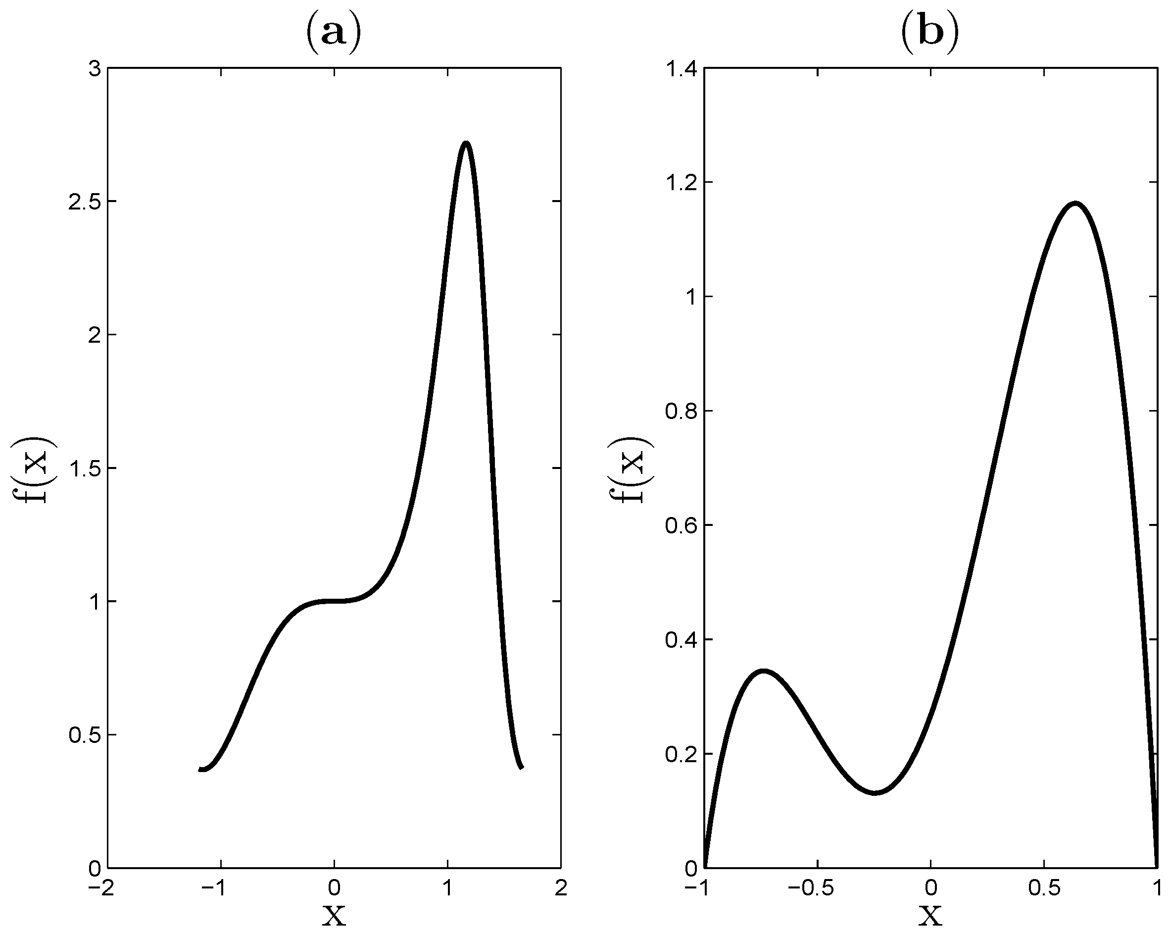
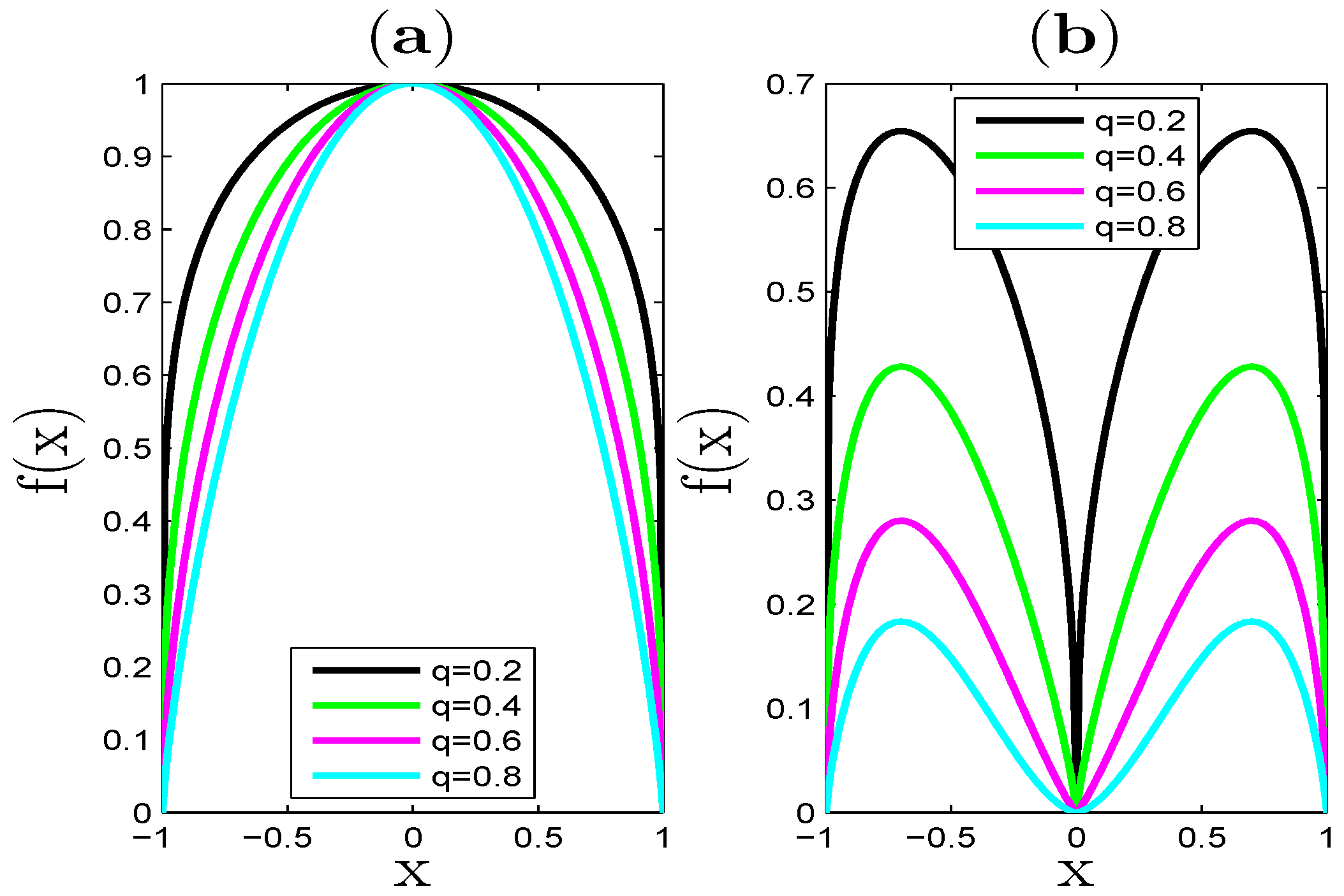
Suppose that we have measurement functions in Equations (8)–(11). These functions are used for the simulation. They can represent biological objects. They are given with the following forms, and the function f has positive values for each value of variable x, namely .
where q is a parameter of the smoothness constant.
and
They represent the area measured on the each slice of three-dimensional biological objects. The measurement functions in Equations (8) and (11) are used by [9,33], respectively. Each function f and its covariogram function can be an example for the representation of q, even though the function f does not have the parameter q. The two approximately same functions can be proposed, , where , , which have different mathematical expressions; however, they can be a neighborhood of each other. For example, the measurement functions in Equations (10) and (11) can be a more modified version of in Equation (9). in Equation (9) can be a modified version of in Equation (8).
Since the covariogram functions of measurement functions in Equations (8)–(11) (displayed by Figure 1 and Figure 2) cannot be calculable to get the integral values, a model for the covariogram functions should be proposed. In this sense, the covariogram functions can be modeled by a polynomial with the fractional power,
2.1.3. Approximate Variance of
By using Equation (5) and the properties of , we finally get:
(detailed expressions are given in Ref. [6,7,8,9]).
The Fourier transformations of parts and in the covariogram model in Equation (12) are zero. Thus, the variance extension term of systematic sampling on is obtained by using the formula given in Equations (9.1) and (9.2) in [8] as follows,
which is the Fourier transformation of for the one-dimensional systematic sampling. .
By using Equations (12)–(14), Equation (15) is obtained.
where
Γ, ζ are Gamma and Riemann’s Zeta functions in [34], respectively. is unbiased point estimators of ,
Equation (16) is obtained according to Fourier transformation basically given in [8]. However, Equation (18) is obtained according to the generalized version of the refined Euler–MacLaurin, proposed by [9].
Note that Equations (16) and (18) give the same results, because the connection between the generalized version of the refined Euler–MacLaurin summation formula and Matheron’s transitive theory is expressed by [9].
We calculate the estimated coefficient of error for the systematic sampling on by means of Equation (20) given below,
where
This is defined to be a coefficient of error of Matheron’s covariogram model. Equations (6) and (21) have in fact inheritance. observations are required due to Equation (21) [6,7,8,9,17,20,21].
The estimation values of parameter q from , , and measurement functions will be obtained at the simulation section. The works in Ref. [1,2,3,4,5,6,7,8,9,10,11,13,14,16,17,18,19,20,21,22,23,24,25,26,27,28,29,30,31] used the covariogram model for the different measurement functions. We aim to show the performance of the covariogram model in Equation (12) for the different measurement functions. In other words, the capability of the covariogram model for fitting performance on the covariogram functions is tested, so the information gained by this model is displayed by the simulation results. By using this model and the variance extension term in Equation (15), the estimation formula of parameter q is given in the following subsection.
2.1.4. Estimation Formula of Parameter q
The estimation formula of smoothness constant q is proposed by [9]. In this subsection, we will get it via the variance extension term in Equation (15) in the framework of the Fourier transformation. The formula we got for q is the same as the formula in [9].
The covariogram model g can be declared by integer k values. If is near zero, Equation (7) has more information. By using Equations (12) and (15), respectively,
can be obtained. By using Equations (19) and (22),
is obtained and then:
where,
By using Equation (17),
The estimator is obtained when the is obtained by planimetry. The planimetry is also called automatic pixel counting given in the section for real data.
2.2. Confidence Interval in Systematic Sampling on ℝ
We will give an exact calculation of in a generalized version of the refined Euler–MacLaurin summation formula with a fractional power of measurement functions. A brief introduction and some tools will be given in the next subsection to get the formula of for the confidence interval of .
2.2.1. Confidence Interval of :
Some definitions expressed in Ref. [2,9] will be given. A theorem will be proposed for a tool in the constant .
A bounded interval for the difference , which is defined as a generalized version of the refined Euler–MacLaurin summation formula, is:
where
and . is the set of a real line at which function exhibits discontinuities. N is the number of sets. The difference and are given by Equations (6) and (11) in Ref. [2]. If N is greater than 2, the information in decreases (for detailed expressions, see Ref. [2]). The preliminaries were given. Now, we will use the tools in Ref. [2,9]. After some straightforward calculations in the following steps, the formula of will be obtained.
By means of the Cauchy–Schwarz inequality , where ,
When Equations (26) and (28) are used,
is obtained.
When in Equation (30) is written in Equation (29), Equation (31) is obtained.
is a function of q and N. In the following steps, we will give a definition for the function in [34]. The function in Equation (27) is required to apply Theorem 1 for the exact calculation of .
From Equation (31), for true parameter Q, a bounded interval (or confidence interval) is given as [2,3]:
From Equation (34), is obtained,
We will give the following theorem to get the values exactly.
Theorem 1.
- 1.
- Supposing that we have a right-open side interval , the maximum value of the interval is:
- 2.
- Supposing that we have a left-open side interval , the maximum value of the interval is:
- 3.
- Supposing that we have a left-open side and right-open side interval , the maximum value of the interval is:
In order to calculate in Equation (27) exactly, Δ is replaced with , because we must take the maximum value of Δ. When , we get the result for the function given in the following form,
Now, we can explain how to get the values of constant below. In the following lines, we will give the limit values done by Mathematica 7, 8 or 9.
When N and given in Equation (32) are replaced with 2 and Equation (35), respectively, we get an equation,
The codes written in Mathematica 7 or higher versions 8 and 9 do not compute the value of and give infinity. Therefore, for the calculation of , we use Equation (38) in order to give the result.
By means of Equation (37), we get :
By using Equation (37), for ,
is obtained. For other q values, a similar procedure is performed. By using the formula given in Equation (32), the values in Table 1 are obtained for and [35].
It is attested that and give the same values for , which is used to define the right-open side interval.
2.2.2. Exact and Computational Values of
We got the values of for different q and N values by using the exact calculation. This calculation was done by the Mathematica 7 or the higher Versions 8 and 9. One can get the values of for the different q values with , and . When the number of sequences in codes prepared by [2] is increased, the computational values of converge to the exact values of (see Table 1 and Table 2). Because getting the computational values of for would be unlikely to be useful, we give up computing some of them. : the number of sequences increased by a user, .
3. Results
This section will give the simulation results for the estimation of parameter q in the variance extension term in Equation (20). Together with the estimated with for Equations (8)–(11), it is planned to see whether or not the confidence interval includes the true value of volume. While constructing the confidence interval, the approximate variance based on Matheron’s covariogram model and the empirical true variance estimations are used. Real data examples are given to test the performance of the confidence interval.
3.1. Simulation
3.1.1. Plan and Output of Simulation
, , and are the abbreviations for the coefficient of error of Matheron’s covariogram model, the coefficient of error for the empirical true variance, the coverage probability of confidence interval based on the coefficient of error for the Matheron’s covariogram model and the coverage probability of confidence interval based on the coefficient of error for the empirical true variance, respectively. The last two abbreviations are for the coverage probabilities of confidence intervals based on and . If the true value Q is in the confidence interval, the confidence interval is successful. The numbers of successes for each replication of sampling are counted and divided by the number of replications. Thus, the values of the coverage probability of the confidence interval for a parameter Q are computed. and are the simulated variance and the simulated mean squared error of the estimator , respectively. The k in q formula was taken to be two, because must be near zero in order to increase the information in Equation (7).
In the simulation performed, the number of replication is 3000, and the numbers of systematic samplings, n, on are from 5–20 for the measurement functions in Equations (8)–(11). The number of systematic samplings is taken to be 20 at most for practical purposes.
The following lines represent the produced x values of , the values of , the estimated values of parameter Q and the coefficient of error for the empirical true variance in three blocks given below.
FOR i FROM 1 TO the number of replication
 FOR j FROM 0 TO the number of systematic sampling minus one
  T(j)=Length of interval of domain of function / the number of systematic sampling
 FOR k FROM 1 TO the number of systematic sampling
   x(k,j,i)=Left end point of the domain of the measurement function+(u(j,i)+j)T(j)
   y(k,j,i)=Measurement function(x(k,j,i))
 END FOR
 END FOR
END FOR

FOR i FROM 1 TO the number of replication
 FOR j FROM 1 TO the number of systematic sampling
   Estimated Q in replicated sampling=(Summation of y in replicated sampling)T(j)
 END FOR
END FOR

FOR i FROM 1 TO the number of systematic sampling
 Summation of empirical variance in each number of systematic sampling is assigned to be zero
 FOR j FROM 1 TO the number of replication
   Empirical variance in each replication=(Estimated Q in each replication-True value)^2;
   Summation of empirical variance in each replication
 END FOR
 Mean of empirical variance=Summation of empirical variance in each replication/The number of replication
 The coefficient of error for the empirical true variance=The root of mean of empirical variance/True value
END FOR
3.1.2. Estimations for Parameter q and Variance Approximation of
As implied by p. 319 in [8], it is obvious that the changing of affects the variance extension term given in Equation (15). In this sense, the covariogram model in Equation (12) can be adopted for some measurement functions. The simulation results in Table A1, Table A2, Table A3, Table A4, Table A5, Table A6, Table A7, Table A8, Table A9, Table A10, Table A11 and Table A12 show that the covariogram model can be used for the measurement functions given in Equations (8), (9) and (11). Note that the integral of the function in Equation (9) is computed by means of the numerical integration in MATLAB , but the integrals of the functions in Equation (8), (10) and (11) are computed by means of the ‘int’ function, which is a function for the exact calculation of the integral in MATLAB . The covariogram model in Equation (12) is proposed intuitively by [6,7]. We want to use it to check the performance of variance estimation in Equation (20). By using the covariogram model in Equation (12), the estimation of q can be said to be an open problem for the measurement functions in Equations (8)–(11), except Equation (8) with . It is observed from the simulation results that the performance of the q formula depends on the covariogram model in Equation (12) and the variance extension term in Equation (20). For irregular , such as Equations (10) and (11), the estimations of q are unstable, namely, they change according to the sample size. It should be noted that for each sample size, the information on the equidistant systematic sampling version of f changes. When we have regular patterns, such as Equations (8) and (9), the estimations of q are stable according to the sample size.
Suppose that we have a flexible balloon filled with gas. This three-dimensional balloon can have different shapes after modification done by hand. Thus, each measurement function can be in a class for the functions with parameter q. As is seen, Equations (10) and (11) do not have the parameter q, but we want to estimate it to get the values of variance estimation precisely for them. The true parameter values of them are accepted to be , respectively, because it seems that the estimated values of parameter q are around these values under Equations (12) and (20).
The estimated values for q of the measurement functions in Equation (8) with and also Equation (9) with and would be around the true parameter values. It is seen that the covariogram model in Equation (12) cannot be a very good representative for these q values of two measurement functions. However, when it is considered on the performance of variance estimation, the values of and for the systematic sampling of Equations (8), (9) and (11) contain the same numbers of zero digits in the fraction part the most times under Equations (12) and (20). It should be noted that even though in Equation (11) does not have the parameter q, the values of and contain the same number of zeros in the fraction part when the sample sizes are from 6–20. When , there is not enough information due to the irregular form of . It is seen from the simulation results that the values of for in Equation (11) are more approximate than that of Equations (8) and (9) generally, which shows evidence that we can propose a function without a parameter q, which is a neighborhood of functions with parameter q. In other words, we have a family for the covariogram functions. This family can be modeled by the covariogram model. This is one of the reasons why the proposed must be used. The efficiency for the systematic sampling of in Equation (10) is not as good as that of Equation (11) because of Equations (12) and (20). The covariogram function of Equation (10) cannot be modeled by the covariogram model. The precision of the systematic sampling of in Equation (10) should be improved. This shows us that the proposed measurement functions are also used while making research into the applied science when Equation (20) is used. As a result, for Equations (8), (9) and (11), Equations (12) and (20) give the values around ; however, for Equation (10), the values of and do not contain the same number of zero digits in the fraction part even if the sample size increases. The fluctuation of is an expected result, because the idea of estimation for parameter Q via the systematic sampling in Equation (1) is used.
3.1.3. Confidence Interval of : Empirical True and Approximation for
The theoretical coverage probability of the confidence interval for a parameter Q was . In this sense, the coverage probabilities of confidence intervals based on the coefficient of error for Matheron’s covariogram model are ; but the coverage probabilities of the confidence intervals based on the coefficient of error for the empirical true variance cannot be . It is observed that the coverage probabilities of confidence intervals based on the coefficient of error for the empirical true variance are approximately. The benefit of using the covariogram model with parameter q is that the bandwidth of confidence can be more accurate for a class of measurement functions, such as Equations (8), (9) and (11).
3.1.4. Confidence Interval of :
can be approximated to for Equations (8), (9) and (11), and so, the coverage probabilities of the confidence intervals based on and , which are called and , respectively, can be considered to have similar values, which shows that our investigation on the performance of values is reasonable. In other words, when we look at the performance of the confidence interval for whether or not it includes the true value, we should focus on and , which must give similar results together. To this point, the trustiness of the confidence interval is acceptable, because is at least approximately. In all performed simulations, N in is taken to be two, which shows us that the confidence interval keeps itself in the optimal sense. This optimality is supported by and , because they have similar results. In other words, suppose that if N is taken to be three, the bandwidths of the confidence interval in the case are larger than that of . In such a case, we would have non-useful information for the confidence band of . Another point we should focus on is the values in Table 1 and Table 2, because the exact values of constant provide useful information for the confidence band. For in Equation (10), since is , it seems the constant produces the confidence intervals, which includes the true value of the area. However, the accurateness of the constant with the empirical true variance and the approximate variance estimations should be examined together. For the same values of , the bandwidths of the confidence intervals with are smaller than that of , which shows us that the bandwidths of confidence intervals constructed with are more accurate than those of . When we look at Table A12, and have the same values, except that the number of samplings n is equal to five. The more number of samplings means the more information gained from the . This is one of the reasons why the proposed must be used. For in Equation (11), it is important to take a value for q, such that we can not only estimate the variance of systematic sampling more precisely, but also choose the right value for the constant . Finally, proposing a class of measurement functions for research helps us to control the trustworthiness of the research in the applied science if the experts in the area can propose them correctly.
A final comment for the simulation section is that the covariogram model in Equation (12) and the variance extension term in Equation (20) can be used. However, the proposed measurement functions, such as Equations (8)–(11), should be systematically sampled, so that one can get a more precise decision on the application for biomedical imaging. As another solution, Equation (20) may be reformulated in the framework of the fractional Fourier transformation proposed by [36,37].
3.2. Real Data
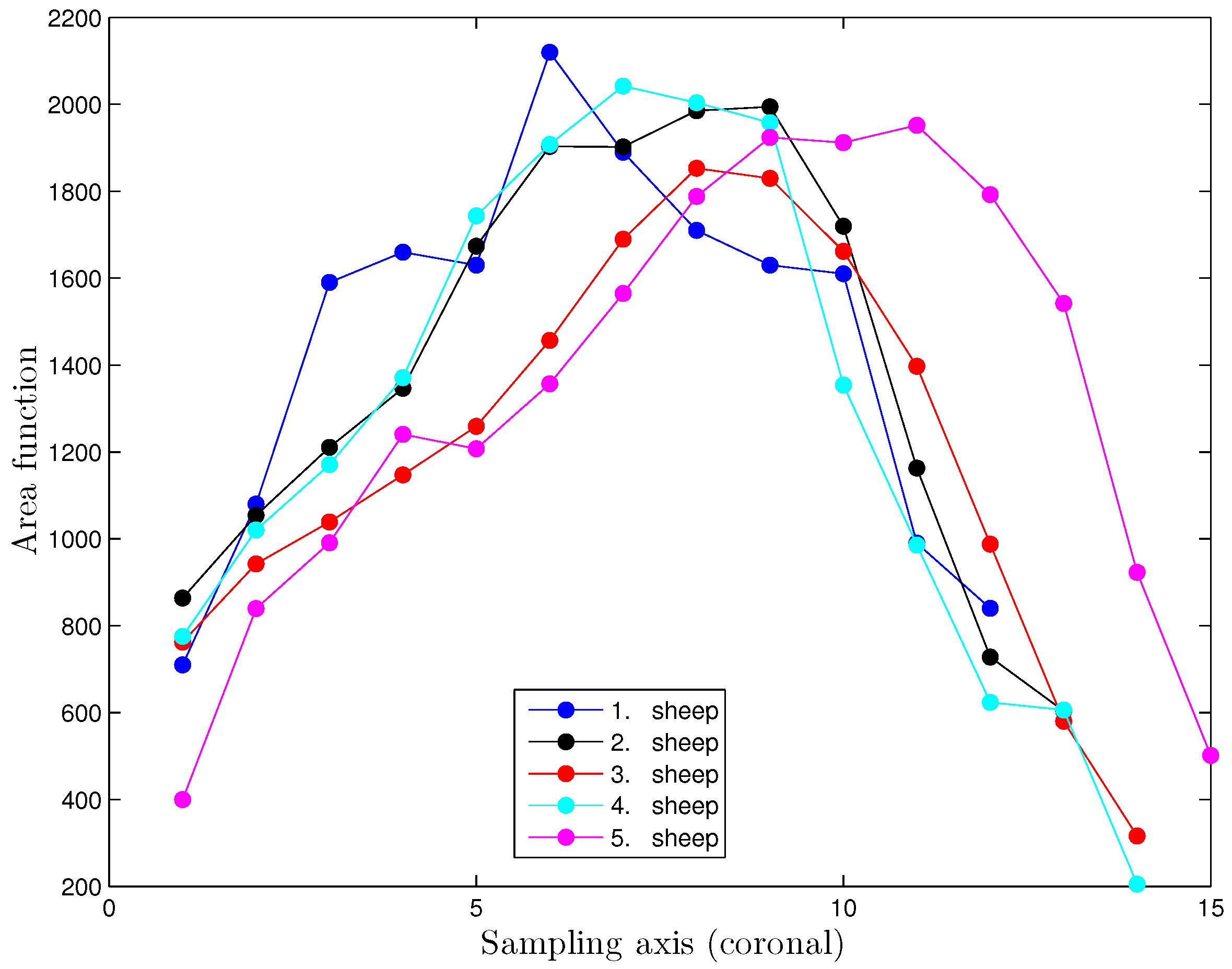
Five different sheep brains, which were 12–18 months old, were removed from their skull via craniotomy in the laboratory for anatomy. These brains were immersed in formalin (5%) for 10 days. Brains were scanned with standard -weighted Tesla magnetic resonance imaging (MRI) in the coronal plane with a 5-mm slice thickness. The true values of volume for each brain were obtained by using the Archimedean principle repeated six times. The arithematic mean of six results for each brain was used as a true value of the volume of a brain. After MRI scanned the sheep brains, the area of each digital image for slices of brains was computed by pixel counting. While doing the pixel counting, the edges of each digital image were detected by experts in the anatomy area. After that, they were estimated by the slices in the coronal plane. The results are given in Table 3 and Table 4. Table 3 and Table 4 show the true values for the volume (Q), the estimated volume (), the estimated smoothness constant (), the estimated coefficient of error (), the lower bound of the estimated volume (), the upper bound of the estimated volume () and the number of slices (Num. Slc.). The area values of each slice obtained from the coronal axis are depicted in the Figure 3.
When N in Equation (32) is replaced with three, and are found. The confidence intervals of Brain 2 for and are (87,055.68, 94,420.32) and (86,981.44, 94,494.56), respectively. These confidence intervals include the true value of volume for Brain 2.
In Table 4, when the estimated with is taken, the confidence interval includes the true values of volume for each non-vivo brain. It is seen that estimating accurately the parameter q affects the variance estimation and the confidence interval, as well. For this reason, values for in Table 1 are computed. The simulation results show that N should be two. The more precise measurement of the slice area is needed for the real data case, because measuring the area of slices more precisely produces the shape of more accurately. Having a more accurate shape of means that the estimated values of parameter q can be determined more accurately. However, it should be noted that the estimation of parameter q except Equation (8) with is an open problem, as well, even if the exact form of is known. Taking the values of k in q formula and N in the constant as bigger than two is not useful due to the loss of information; however, we do not have a solution for the real data case. In the real data case, we have to try different values of k and N, and also, the proposed must be used to increase the trustworthiness of research in the applied science. As a result, using two propositions is required.
4. Conclusions and Discussions
The works in Ref. [6,7,8,9,10,11,12,13,14,15,19,20,21,22] focused on the variance estimation for systematic sampling. As implied by [9,17,21], the estimation of q is important to avoid the biasedness of the variance estimator in systematic sampling on . The unbiasedness of the variance extension term estimator leads to having accurate lower and upper bounds of the confidence interval for the systematic sampling on . In fact, the true variance in Equation (5) is the combination of three components, so we always have biased variance estimation; however, for practical purposes, we are only interested in the variance extension term. It is observed from the simulation results that and have values that contain the same number of zero digits in the fraction part for the measurement functions in Equations (8), (9) and (11) at most times under Equations (12) and (20). However, the same performance of the formula in Equation (20) is not observed for the variance approximation of the systematic sampling of in Equation (10) even if the number of sample sizes increases. Therefore, the formulae in Equation (12) and Equation (20) are not appropriate to use. It should be noted that due to the definition of systematic sampling given in Equation (1), a fluctuation can be observed, so evaluating the performance of and according to the behavior of the sample size cannot be sensible. However, when the sample size increases, it is logical to expect the information coming from to be increased. In this context, Table A1, Table A2, Table A3, Table A4, Table A5, Table A6, Table A7, Table A8, Table A9, Table A10, Table A11 and Table A12 show that when the sample size increases, the values of and are decreased. As implied by p. 319 in [8], if a measurement function has irregularities, such as Equations (9)–(11), the values of are high when the sample size is small, because the information is not enough to catch the approximate shape of the three-dimensional object. For the measurement functions in Equations (9)–(11), Table A6, Table A8, Table A10 and Table A12 support this implication on p. 319 of [8]. The values of in Equation (9) with can approve the fluctuation when the sample sizes are 5–20. For other measurement functions, the fluctuation on is not observed; in fact, there is a fluctuation; however, the effect of sample size covers the fluctuation. Otherwise, proposing a Fourier transformation to model the estimated values of parameter Q would not give the results for that are approximate to .
A three-dimensional object is represented by a flexible balloon filled with gas. The shape of this balloon can be modified by means of hands. The volume of the balloon can change after each modification; however, it is not important whether or not there is a change of the volume of the balloon. The modified versions of the balloon are represented by the measurement functions given in Equations (8)–(11). The measurement functions in Equations (10) and (11) do not have the parameter q; however, they can be a neighborhood of having parameter q. Since we have different forms of the balloon, we will have many forms of the measurement functions representing the three-dimensional object exactly. In the real data case, knowing the exact form of the three-dimensional object is impossible. The covariogram functions coming from the without q will be the neighborhood of the covariogram functions coming from with q. This is why the covariogram model has the parameter q. The true with q cannot be known exactly due to fact that we can have without q, which is a neighborhood of with q. In other words, we can have approximately the same functions, which are different mathematical expressions.
A method showing how to calculate constant is proposed. It is expected that this method can be used as a new tool in mathematics when it is needed. A package program written in MATLAB gives the lower and upper levels of confidence and the quantitative values of stereology when the data obtained from a single replication is typed. The program can be supplied on request. The estimation of q is an open problem, even if we know the exact form of the measurement functions, except Equation (8) with . In the other perspective of our discussion, the covariogram model cannot be a very good approximation for the covariogram functions of measurement functions. However, the values of and contain the same numbers of zero digits in the fraction part at most times for the measurement functions in Equations (8), (9) and (11) under Equations (12) and (20).
The values of and are the other criteria to approve the performance of the exact values of the constant , as observed from the simulation results. A numerical computation for the constant of the confidence interval was done by [2]. The more precise the values of the constant means the more precise the confidence interval. It is obvious that the proposition of exact calculation has to be preferred, because the computation of the constant proposed by [2] is not as good as the results displayed by Table 1 and Table 2, as seen by the conformity between and for exact values of , especially for the measurement functions in Equations (8), (9) and (11).
It is observed that the synthetic data can approve the real data for non-vivo brains if the real data have an exactly similar form as the synthetic data. Since the real data cannot be represented by the exactly similar measurement functions, we should prefer to use different N values. For this reason, we chose the different k values for the estimation of q in real data. Equation (25) can produce the negative estimated value for the area function of the real data given in Figure 3. The constant values for different N values must be given, because the real data shows that we need constant values with different N. In this context, the edges of digital images have to be found more precisely. Especially, when the edges of images are more irregular, the precision of getting area values for each image has to be decreased significantly. To do this, new edge detection methods proposed by [38] can be used.
The proposed measurement functions should be systematically sampled while conducting research on biomedical imaging to increase the information in the decision rule for now. To be able to increase the performance of the variance approximation, the fractional Fourier transformation may be applied to get a new variance estimation of the equidistant systematically sampled on . Other types of may also be used. In this case, we need the computational integral techniques. The studies done by [39,40] will be enlightening for the computational integration of other types that we will use. For the construction of via digital images, which have coronal, axial or sagittal directions, the new edge detection methods proposed by [38] may be applied to get more precise area values of slices. We will prepare a free statistical software R package with a macro for Mathematica for all methodologies given here and in the future.
Acknowledgments
I am very grateful to Luis M. Cruz-Orive who sincerely invited me, to Marta García-Fiñana for sending the codes in R and to Niyazi Acer for kindly providing the data. I am also so indebted to the Council of Higher Education for giving the funding for my research. I am indebted to James F. Peters from the University of Manitoba, Winnipeg, Canada, for critical reading. I would like to thank sincerely the four referees. Without their help, this paper would not have been improved. I also wish to thank my great parents. In the memory of my great brother.
Author Contributions
Mehmet Niyazi Çankaya finished the manuscript. The author has read and approved the final manuscript.
Conflicts of Interest
The author declares no conflict of interest.
Appendix A

| n | |||
|---|---|---|---|
| 5 | |||
| 6 | |||
| 7 | |||
| 8 | |||
| 9 | |||
| 10 | |||
| 11 | |||
| 12 | |||
| 13 | |||
| 14 | |||
| 15 | |||
| 16 | |||
| 17 | |||
| 18 | |||
| 19 | |||
| 20 |
| n | ||||
|---|---|---|---|---|
| 5 | ||||
| 6 | ||||
| 7 | ||||
| 8 | ||||
| 9 | ||||
| 10 | ||||
| 11 | ||||
| 12 | ||||
| 13 | ||||
| 14 | ||||
| 15 | ||||
| 16 | ||||
| 17 | ||||
| 18 | ||||
| 19 | ||||
| 20 |
References
- Eriksen, N.; Rostrup, E.; Andersen, K.; Lauritzen, M.J.; Larsen, V.A.; Dreier, J.P.; Strong, A.J.; Hartings, J.A.; Fabricius, M.; Pakkenberg, B. Application of stereological estimates in patients with severe head injuries using CT and MR scanning images. Br. Inst. Radiol. 2010, 83, 307–317. [Google Scholar] [CrossRef] [PubMed]
- García-Fiñana, M. Confidence intervals in Cavalieri Sampling. J. Microsc. 2006, 222, 146–157. [Google Scholar] [CrossRef] [PubMed]
- García-Fiñana, M.; Keller, S.S.; Roberts, N. Confidence Intervals for the Volume of Brain Structures in Cavalieri Sampling with Local Errors. J. Neurosci. Methods 2009, 179, 71–77. [Google Scholar] [CrossRef] [PubMed]
- Hussain, Z.; Roberts, N.; Whitehouse, G.H.; García-Fiñana, M.; Percy, D. Estimation of Breast Volume and its Variation During the Menstrual Cycle using MRI and Stereology. Br. J. Radiol. 1999, 72, 236–245. [Google Scholar] [CrossRef] [PubMed]
- McNulty, V.; Cruz-Orive, L.M.; Roberts, N.; Holmes, C.J.; Gual-Arnau, X. Estimation of Brain Compartment Volume from MR Cavalieri Slices. J. Comput. Assist. Tomogr. 2000, 24, 466–477. [Google Scholar] [CrossRef] [PubMed]
- Matheron, G. Variables Régionalisées et Leur Estimation [Les]; Masson: Paris, France, 1965. [Google Scholar]
- Matheron, G. The Theory of Regionalized Variables and Its Applications. In Les Cahires du Centre de Morphologie Mathématique de Fontainebleau, No. 5; Ecole Nationale Supérieure des Mines de Paris: Paris, France, 1971. [Google Scholar]
- Cruz-Orive, L.M. On the Precision of Systematic Sampling: A Review of Matheron’s Transitive Methods. J. Microsc. 1989, 153, 315–333. [Google Scholar] [CrossRef]
- García-Fiñana, M.; Cruz-Orive, L.M. Improved Variance Prediction for Systematic Sampling on R. Statistics 2004, 38, 243–272. [Google Scholar] [CrossRef]
- Gual Arnau, X.; Cruz-Orive, L.M. Variance prediction under systematic sampling with geometric probes. Adv. Appl. Probab. 1998, 30, 889–903. [Google Scholar] [CrossRef]
- Gundersen, H.J.G.; Jensen, E.B. The Efficiency of Systematic Sampling in Stereology and its Prediction. J. Microsc. 1987, 147, 229–263. [Google Scholar] [CrossRef] [PubMed]
- Kellerer, A.M. Exact formulae for the precision of systematic sampling. J. Microsc. 1989, 153, 285–300. [Google Scholar] [CrossRef] [Green Version]
- Kiêu, K. Three Lectures on Systematic Geometric Sampling; Memoirs 13; Department of Theoretical Statistics, University of Aarush: Aarhus, Denmark, 1997; p. 100. [Google Scholar]
- Kiêu, K.; Souchet, S.; Istas, J. Precision of Systematic Sampling and Transitive Methods. J. Stat. Plan. Inference 1999, 77, 263–279. [Google Scholar] [CrossRef]
- Mattfeldt, T. The accuracy of one-dimensional systematic sampling. J. Microsc. 1989, 153, 301–313. [Google Scholar] [CrossRef]
- Roberts, N.; Cruz-Orive, L.M.; Reid, M.K.; Brodie, D.A.; Bourne, M.; Edwards, H.T. Unbiased Estimation of Human Body Composition by the Cavalieri Method Using Magnetic Resonance Imaging. J. Microsc. 1993, 171, 239–253. [Google Scholar] [CrossRef] [PubMed]
- García-Fiñana, M.; Cruz-Orive, L.M.; Mackay Clare, E.; Pakkenberg, B.; Roberts, N. Comparison of MR Imaging Against Physical Sectioning to Estimate the Volume of Human Cerebral Compartments. NeuroImage 2003, 18, 505–516. [Google Scholar] [CrossRef]
- Baddeley, A.J.; Vedel Jensen, E.B. Stereology for Statisticians; Monographs on Statistics and Applied Probability; Chapman & Hall/CRC: London, UK, 2005; p. 380. [Google Scholar]
- Cruz-Orive, L.M. Variance predictors for isotropic geometric sampling, with applications in forestry. Stat. Methods Appl. 2012, 22, 3–31. [Google Scholar] [CrossRef]
- Cruz-Orive, L.M. Systematic Sampling in Stereology. In Proceedings of the 49th Session of the International Statistical Institute, Florence, Italy, 25 August–3 Sepetmber 1993; Volume 55, pp. 451–468.
- Cruz-Orive, L.M. A General Variance Predictor for Cavalieri Slices. J. Microsc. 2006, 222, 158–165. [Google Scholar] [CrossRef] [PubMed]
- Gundersen, H.J.G.; Jensen, E.B.V.; Kiêu, K.; Nielsen, J. The Efficiency of Systematic Sampling in Stereology—Reconsidered. J. Microsc. 1999, 193, 199–211. [Google Scholar] [CrossRef] [PubMed]
- Acer, N.; Şahin, B.; Usanmaz, M.; Tatoǧlu, H.; Irmak, Z. Comparison of Point Counting and Planimetry Methods for the Assessment of Cerebellar Volume in Human Using Magnetic Resonance Imaging: A Stereological Study. Surg. Radiol. Anat. 2008, 30, 335–339. [Google Scholar] [CrossRef] [PubMed]
- Acer, N.; Şahin, B.; Emirzeoğlu, M.; Uzun, A.; İncesu, L.; Bek, Y.; Bilgiç, S.; Kaplan, S. Stereological Estimation of the Orbital Volume: A Criterion Standard Study. J. Craniofacial Surg. 2009, 20, 921–938. [Google Scholar] [CrossRef] [PubMed]
- Acer, N.; Çankaya, M.N.; İşçi, Ö.; Baş, O.; Çamurdanoğlu, M.; Turgut, M. Estimation of Cerebral Surface Area using Vertical Sectioning and Magnetic Resonance Imaging: A Stereological Study. Brain Res. 2010, 1310, 29–36. [Google Scholar] [CrossRef] [PubMed]
- Akbaş, H.; Şahin, B.; Eroğlu, L.; Odacı, E.; Bilgiç, S.; Kaplan, S.; Uzun, A.; Ergür, H.; Bek, Y. Estimation of Breast Prosthesis Volume by the Cavalieri Principle Using Magnetic Resonance Images. Aesthet. Plast. Surg. 2004, 28, 275–280. [Google Scholar] [CrossRef] [PubMed]
- Howard, M.A.; Roberts, N.; García-Fiñana, M.; Cowell, P.E. Volume Estimation of Prefrontal Cortical Subfields using MRI and Stereology. Brain Res. Protoc. 2003, 10, 125–138. [Google Scholar] [CrossRef]
- Maudsley, R.; García-Fiñana, M. Sampling Intensity with Fixed Precision When Estimating Volume of Human Brain Compartments. Image Anal. Stereol. 2008, 27, 143–149. [Google Scholar] [CrossRef]
- Roberts, N.; Pubdephat, M.J.; McNulty, V. The Benefit of Stereology for Quantitative Radiology. Br. J. Radiol. 2000, 73, 679–697. [Google Scholar] [CrossRef] [PubMed]
- Şahin, B.; Emirzeoğlu, M.; Uzun, A.; İncesu, L.; Bek, Y.; Bilgiç, S.; Kaplan, S. Unbiased Estimation of the Liver Volume by the Cavalieri Principle Using Magnetic Resonance Images. Eur. J. Radiol. 2003, 47, 164–170. [Google Scholar] [CrossRef]
- Şahin, B.; Ergür, H. Assessment of the Optimum Section Thickness for the Estimation of Liver Volume Using Magnetic Resonance Images: A Stereological Gold Standard Study. Eur. J. Radiol. 2005, 57, 96–101. [Google Scholar] [CrossRef] [PubMed]
- Bellhouse, D.R.; Krishnaiah, P.R.; Rao, C.R. (Eds.) Sampling: Handbook of Statistics; Elsevier Science: Amsterdam, The Netherlands, 1988; Volume 6, pp. 125–145.
- Hall, P.; Ziegel, J. Distributions estimators and confidence intervals for stereological volumes. Biometrika 2011, 98, 417–431. [Google Scholar] [CrossRef]
- Abramowitz, M.; Stegun, I.A. Handbook of Mathematical Functions; U.S. Government Printing Office: Washington, DC, USA, 1970; p. 1058.
- Çankaya, M.N. Stereological Estimation and Inference with Applications. Master’s Thesis, Council of Higher Education, Ankara, Turkey, 2010; p. 168. [Google Scholar]
- Baleanu, D.; Wu, G.C.; Duan, J.S. Some Analytical Techniques in Fractional Calculus: Realities and Challenges. In Discontinuity and Complexity in Nonlinear Physical Systems; The Series Nonlinear Systems and Complexity; Springer: Heidelberg, Germany, 2013; Volume 6, pp. 35–62. [Google Scholar]
- Poularikas, A.D. Transforms and Applications Handbook, 3rd ed.; CRC Press, Taylor and Fracis Group: Boca Raton, FL, USA, 2010. [Google Scholar]
- Peters, J.F. Computational Proximity Excursions in the Topology of Digital Images; Intelligent Systems Reference Library; Springer: Basel, Switzerland, 2016; Volume 102, p. 433. [Google Scholar]
- Qin, Y.M.; Shi, Y.G. A new approximate method to conjugacies between a family of unimodal interval maps. J. Comput. Complex. Appl. 2016, 2, 163–169. [Google Scholar]
- Zengn, Y. Approximate solutions of three integral equations by the new Adomian decomposition method. J. Comput. Complex. Appl. 2016, 2, 38–43. [Google Scholar]
Figure 1.
Measurement functions with parameter q. (a) Measurement function () of Equation (8); (b) of Equation (9).

Figure 3.
Area functions for each brain.

| q | |||
|---|---|---|---|
| 0 | - | - | |
| 3.32203 | 3.83595 | ||
| 3.59855 | 4.15525 | ||
| 3.82689 | 4.41891 | ||
| 4.004 | 4.62342 | ||
| 4.12699 | 4.76544 | ||
| 4.19345 | 4.84218 | ||
| 4.20165 | 4.85165 | ||
| 4.15073 | 4.79285 | ||
| 4.04079 | 4.6659 | ||
| 1 | 3.87298 | 4.47214 |
| q | ||||
|---|---|---|---|---|
| 0 | 2.418465 | - | - | |
| - | - | - | ||
| - | - | 2.926749 | ||
| 3.105091 | 3.111937 | 3.114245 | ||
| - | - | 3.258353 | ||
| - | - | 3.365038 | ||
| 3.408876 | 3.412577 | 3.414001 | ||
| - | - | 3.426855 | ||
| - | 3.38736 | 3.387638 | ||
| 3.29831 | 3.298648 | 3.298765 | ||
| 1 | - | - | - |
Table 3.
Five sheep brain volumes from automatic pixel counting (mm) after determining the border of slices with a 5-mm thickness and their confidence intervals for : arithmetic mean of values with in Equation (25). Num. Slc., number of slices.
| Brains | Q | Num. Slc. | |||||
|---|---|---|---|---|---|---|---|
| 1 | 85,000 | 87,300 | 0.20 | 0.0234 | 81,289.05 | 93,310.95 | 12 |
| 2 | 94,000 | 90,738 | 0.34 | 0.0106 | 87,731.40 | 93,744.60 | 13 |
| 3 | 83,000 | 84,608 | 0.50 | 0.0066 | 82,722.64 | 86,493.36 | 14 |
| 4 | 88,000 | 88,846 | 0.42 | 0.0087 | 86,318.13 | 91,372.87 | 14 |
| 5 | 100,000 | 99,675 | 0.67 | 0.0039 | 98,351.66 | 100,998.34 | 15 |
Table 4.
Five sheep brain volumes from automatic pixel counting (mm) after determining the border of slices with a 5-mm thickness and their confidence intervals for : values with in Equation (25).
| Brains | Q | Num. Slc. | |||||
|---|---|---|---|---|---|---|---|
| 1 | 85,000 | 87,300 | −0.06 | 0.0234 | 82,646.98 | 91,953.02 | 12 |
| 2 | 94,000 | 90,738 | 0.18 | 0.0131 | 87,249.31 | 94,226.69 | 13 |
| 3 | 83,000 | 84,608 | 0.41 | 0.0075 | 82,464.84 | 86,751.16 | 14 |
| 4 | 88,000 | 88,846 | 0.28 | 0.0105 | 85,934.10 | 91,756.90 | 14 |
| 5 | 100,000 | 99,675 | 0.63 | 0.0041 | 98,283.46 | 101,066.54 | 15 |
© 2016 by the author; licensee MDPI, Basel, Switzerland. This article is an open access article distributed under the terms and conditions of the Creative Commons Attribution (CC-BY) license (http://creativecommons.org/licenses/by/4.0/).
Share and Cite
MDPI and ACS Style
Çankaya, M.N. Propositions for Confidence Interval in Systematic Sampling on Real Line. Entropy 2016, 18, 352. https://doi.org/10.3390/e18100352
AMA Style
Çankaya MN. Propositions for Confidence Interval in Systematic Sampling on Real Line. Entropy. 2016; 18(10):352. https://doi.org/10.3390/e18100352
Chicago/Turabian StyleÇankaya, Mehmet Niyazi. 2016. "Propositions for Confidence Interval in Systematic Sampling on Real Line" Entropy 18, no. 10: 352. https://doi.org/10.3390/e18100352
Note that from the first issue of 2016, this journal uses article numbers instead of page numbers. See further details here.