
Application of Information Theory for an Entropic Gradient of Ecological Sites

Department of Soil and Forest Ecology, Faculty of Forestry, Süleyman Demirel University, Isparta 32260, Turkey
Entropy 2016, 18(10), 340; https://doi.org/10.3390/e18100340
Submission received: 8 June 2016
/
Revised: 1 August 2016
/
Accepted: 16 August 2016
/
Published: 22 September 2016
(This article belongs to the Special Issue Applications of Information Theory in the Geosciences)
Abstract
:The present study was carried out to compute the straightforward formulations of information entropy for ecological sites and to arrange their locations along the ordination axes using the values of those entropic measures. The data of plant communities taken from six sites found in the Dedegül Mountain sub-district and the Sultan Mountain sub-district located in the Beyşehir Watershed was examined in the present study. Firstly entropic measures (i.e., marginal entropy, joint entropy, conditional entropy and mutual entropy) were computed for each of the sites. Next principal component analysis (PCA) was applied to the data composed of the values of those entropic measures. As a result of the first axis of the applied PCA, the arrangement of the sites was found meaningful from an ecological point of view because the sites were located along with the first component axis of the PCA by illustrating the climatic differences between the sub-districts.
1. Introduction
Biodiversity plays important roles in maintaining ecological balance and the health of ecosystems. General interest in biodiversity has grown rapidly in recent decades. This topic was emphasized especially in the Rio Declaration and renewed by the Lisbon Conference in 1998 [1]. Since diversity should be always defined by using indices to measure it [2], entropy-like quantities have long been used as a measure of diversity in the areas of community ecology and environmental biology. Among those quantities, the most popular metric of biodiversity is derived from information theory [3,4,5,6,7,8].
In information theory, marginal entropy, also called Shannon–Bolztman entropy [5] or diversity-based entropy [9], is a measure of the average uncertainty in the random variable. It can be also described as a measure of the average length of a message that would have to be sent to characterize a sample. Joint entropy is a measure of the uncertainty associated with a set of variables while conditional entropy is the entropy of a random variable conditional on the knowledge of another random variable. The other entropic measure of information theory, mutual entropy, is the reduction in the uncertainly of one random variable due to the knowledge of the other. The mutual entropy is symmetric in X and Y and always non-negative and is equal to zero if X and Y are independent [5,10,11].
All entropy quantities of information theory (i.e., marginal entropy, joint entropy, conditional entropy and mutual entropy) can be used to measure the diversity of ecological communities and the values of those entropic measures may be considered for arranging their sites along the ordination axes by using a multi-dimensional statistical technique such as principal component analysis (PCA).
If the sites of ecological communities are able to be arranged in an ecologically meaningful way along the ordination axes by using the numerical data obtained from all entropic measures, then this ordination data means it is a surrogate variable of the multi-dimensional diversity of ecosystems. In this case, this variable may be used as response data to obtain distribution models of biodiversity. Since such response data is much more valuable to describe the diversity of the ecosystems, as usual, its distribution models and maps will be much more valuable for generating and implementing the ecosystem-based management plans.
In light of the explanations given above, a study was conducted (1) to calculate the entropic measures of the plant communities taken from six sites from the Beyşehir Watershed, Turkey, and (2) to examine their distributions along the ordination axes by applying the PCA.
2. Materials and Methods
Beysehir Watershed is located in 38°2′60″ and 37°25′60″ N and in longitude between 31°15′01″ and 31°46′10″ E. It covers an area of 416,723 ha. It is bounded on the west by the Anamas, Dedegul and Kartoz mountains, in the east by Alacadag, Erenkilit and Sultan mountains, in the north by Şarkikaraağaç plains, and in the south by Seyran and Seydişehir mountains. The altitude of Beysehir lake is 1121 m. The highest mountain of the watershed is Dedegul with an altitude of 2993 meters above sea level (m.a.s.l.). West and south parts of the Watershed are underlain mostly by limestone. Limestones are rich in karstic land-forms, i.e., different size poljes, uvalas, dolines and “U”-shaped valleys. North and east parts are underlain mostly by alluvial deposits, marly and marly limestone, schists and trachyandesite. The leading forest vegetation of the watershed area is pure and mixed forest composed of Cedar (Cedrus libani), black pine (Pinus nigra subsp. pallasiana), Taurus fir (Abies cilicica), oaks (Quercus sp.) and Junipers (Juniperus sp.). Soil stoniness and depth vary with topography and parent material. The main soil categories are cambisols, regosols and leptosols [12].
There are two sub-districts in the watershed. Dedegul mountains sub-district (DEDE) is lying in the west and south of Beysehir Lake and Sultan mountain sub-district (SULTAN) is found in the east of the Beysehir Lake. According to the climatic data provided from Yenisarbademli province found in DEDE, the average annual rainfall is 800 mm and, the average annual temperature is 11.04 °C. According to Sarkikaraagac meteorological stations found in SULTAN, the average annual rainfall 477.4 mm and, the average annual temperature 11.2 °C. The dominant winds blow along with the north-east direction. More than 70% of the forest areas have been subjected to over grazing and individual selection in SULTAN whereas less than 40% of the forest areas are degraded in DEDE [12].
Vegetation data taken from the six sites found in Beyşehir Watershed of the Mediterranean region [12] were used for measuring the entropies. Each of all the sites (I–VI) includes nine complexes taken from 2000 to 1200 m.a.s.l. Altitudinal differences among the complexes are equal to 100 m at each site.
Before applications of the formulations of information entropy, firstly, the cover-abundance values of the plants species found in the sites were transformed as follow: 1 means one or few individuals; 2 means occasional and less than 5%; 3 means abundant and with very low cover, or less abundant but with higher cover; in any case less than 5% cover of total area; 4 means very abundant and less than 5% cover; 5 means 5%–12.5% cover, irrespective of number of individuals; 6 means 12.5%–25% cover of total area, irrespective of number of individuals; 7 means 25%–50% cover of total area, irrespective of number of individuals; 8 means 50%–75% cover of total area, irrespective of number of individuals; 9 means 75%–100% cover of total area, irrespective of number of individuals [13].
Secondly, the raw data matrices containing the species (lines) and complexes (columns) were prepared for each of the sites. The cell values occupied by the ordinal (transformed) values of the species were then converted to the proportional values as can be seen in Table 1. Thus, six data matrices were prepared and storied for applications of the formulations of the information theory.
The equations for information entropy [10,14,15] applied to the species-complexes data matrices of the sites are given in Equation (1) through (6).
where X and Y represent the complexes and plant species, respectively. H(X) and H(Y) are the first order (marginal) entropies and p(x) is the probability of occurrence of signal x (the probabilities of total ordinal values of the species found in the complexes) where and, p(y) the probability of occurrence of signal y (the probabilities of the ordinal values of the species) where (Table 1). If the probability is completely uniform then p(x) = 1/N or p(y) = 1/S and then H(X) = log2N or H(Y) = log2S which can be referred to as the “zero order entropy (H0)” [15]. N and S are the number of different signal types. In the present study, N is the number of complexes and S is the number of plants species.
The next entropic measure is the joint entropy H(X,Y) which is defined as:
where p(x,y) is the joint probability. If X and Y are completely independent variables, then H(X,Y) = H(X) + H(Y). If X and Y are not completely uncorrelated, the difference between the joint entropy H(X,Y) and the sum of H(X) and H(Y) would be equal to the mutual entropy (I(X;Y)) which is the measure of the overlapping information transmitted from the two message, and is given by:
The mutual entropy is the measure of uncertainly in the joint occurrence of the combination of X and Y. If some correlation exists between the information in message sets H(X) and H(Y), then the conditional information entropies (H(X|Y) and H(Y|X)), given in Equations (5) and (6), are non-zero.
The sizes of the prepared data matrices (species × complexes) become 30 × 9, 40 × 9, 43 × 9, 18 × 9, 28 × 9 and 24 × 9 from site I to site VI, respectively.
After calculating the entropy values of each of six sites, Pearson correlation analysis was applied among all the entropic measures to examine the relationships with each other. Principal component analysis (PCA) was then applied to the data matrix composed of the values of the entropic measures to observe the positions of the sites along the ordination axes. Correlation analysis and PCA were performed using Paleontological Statistics (PAST) software version 1.89 [16].
3. Results
Using entropic quantities (Equations (1)–(6)), the computed values of entropic measures are given in Table 2.
The zero order entropy (H0) values intended for H(X) of all sites are the same, since all the sites contain equal numbers of complexes, H0(X) = log29 = 3.1699 bits. All the H1(X) values are very close to the H0 values because of two reasons: (1) all sites have the same number of complexes; (2) the distribution of the proportional values (px) of the complexes shows an almost uniform distribution within all sites. Site V has the closest H1(X) value (3.1366 bits) to the maximum entropy value (H0(X)) whereas site I has a value of 3.073 bits, equal to the lowest H1(X) (Table 2).
The H0 values of the sites with the H(Y) term are different from each other due to fact that they have different numbers of species. Since the numbers of the plant species are 30, 40, 43, 18, 28 and 24 from site I to site IV, respectively, H0(YI) = 4.906891, H0(YII) = 5.321928, H0(YIII) = 5.426265, H0(YIV) = 4.169925, H0(YV) = 4.807355 and H0(YVI) = 4.584963. Site III has the maximum H(Y|X), H(X,Y) and H(Y) values. Even though site III has the maximum H(Y) value (Table 2), site V has the closest value to maximum entropy H0(Y). That is probably why site V also has the maximum I(X;Y) value. Since site I has the minimum H(X) and the maximum H(X|Y) values, the I(XI;YI) value of this site has the lowest value corresponding to 0.948 bits (Table 2).
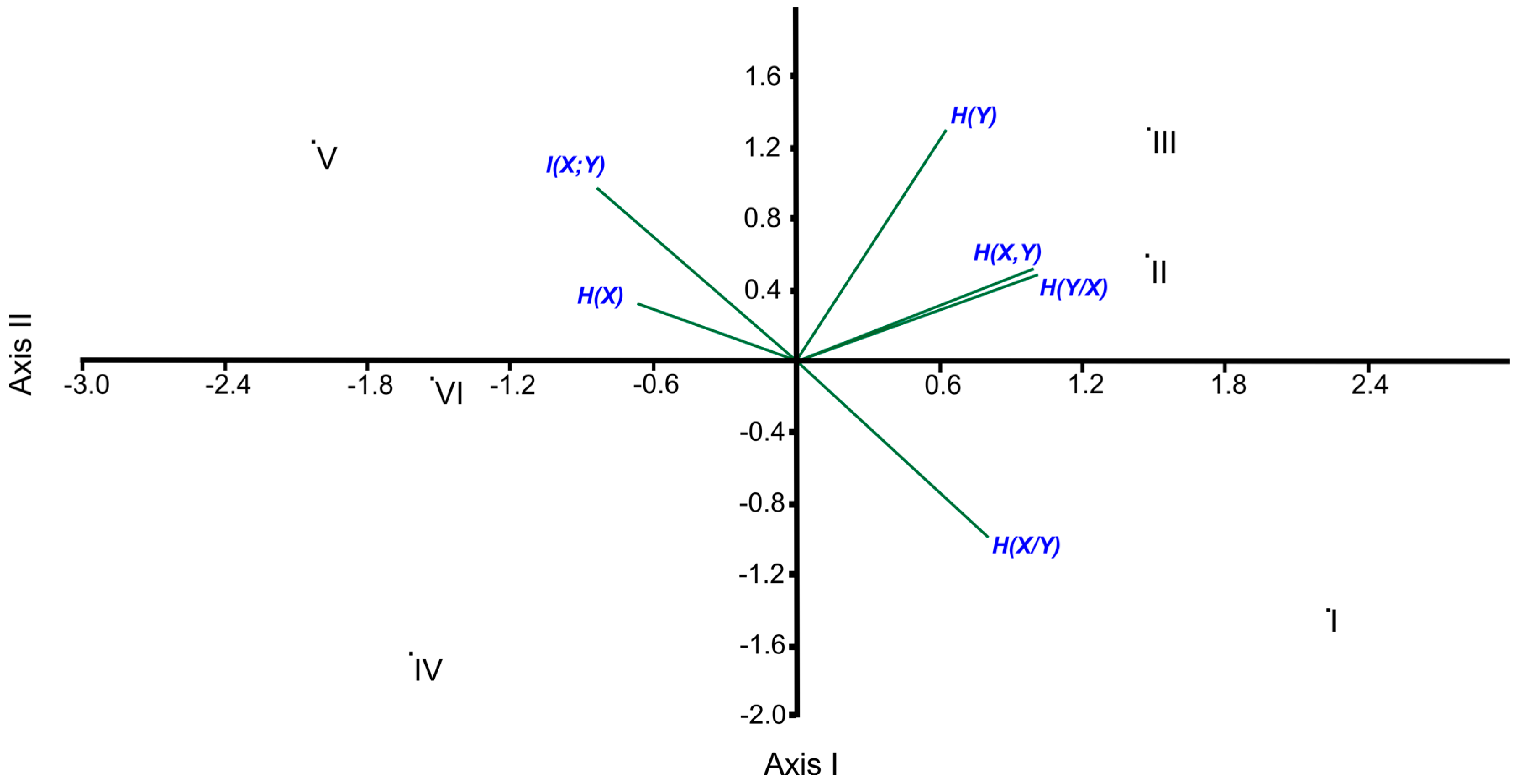
According to the results obtained from the correlation analysis, H(X,Y) shows a parallel trend with H(Y) (r = 0.812, p < 0.05), in particular with H(Y|X) (r = 0.998, p < 0.01). On the contrary, there is a significant negative trend between H(X|Y) and I(X;Y) (r = −0.996, p < 0.01). As a result of the applied PCA, the eigenvalues of the first and the second axes were computed as 3.6868 and 1.6514, respectively, and both of the two axes explained the high percentage of the total variance with a value of 88.97% in which the percentages of explained variances of the first and second axes are 61.45% and 27.52%, respectively. As expected, the locations of the entropic measures along the ordination axes confirm the results of the correlation analyses (i.e., H(X,Y), H(Y) and H(Y|X), which are highly correlated to each other, occupied the upper right, and H(X|Y) was located in the lower right while I (X;Y) was found in the upper left of the ordination diagram due to having a negative significant correlation). Since H(X) has an insignificant association with the other entropic measures, its position is rather close to the center point of the ordination diagram (Figure 1).
The ordination diagram of PCA points out an obvious grouping along the first axis in which the first group contains site I, site II and site III, located at the right, and the second group is composed of site IV, site V and site VI, located at the left, as can be seen in Figure 1.
In the present study, correlation analyses were also applied between the axes’ values and entropic measures. As a result of this, H(X,Y) (r = 0.936 (p < 0.01) between H(X,Y) and Axis I) and H(Y|X) (r = 0.949 (p < 0.01) between H(Y|X) and Axis I) became the most important entropic measures on the distribution of the sites along the first axis.
Even though none of the entropic measures is significantly associated with the second axis, its percentage of explained variance has a considerable value (27.52%). That is why it is necessary to say that the most important entropic measures on the distribution of the sites are H(Y) (r = 0.811, ns), H(X|Y) (r = −0.619, ns) and I(X;Y) (r = 0.610, ns) along the second axis. Note that “ns” means non-significant.
4. Discussion
The grouping of the sites along the first axis is meaningful from an ecological point of view due to following reasons explained below.
In the frame of ecosystem classification, the Beyşehir Watershed is divided into two sub-districts called the Sultan Mountain sub-district (SULTAN) and the Dedegül Mountain sub-district (DEDEGUL). SULTAN is under the impact of the dry and cold winds blowing along from the northeast direction, coming from the inner Anatolian region, where the continental climate is dominant. The drought/semi-drought climatic conditions are, therefore, dominant in SULTAN. However, the climate is humid/very humid in DEDEGUL because the winds blowing along the northeast direction arrive at DEDEGUL by receiving the humid air from above Beyşehir Lake. As a result of this, the forest ecosystems found in DEDEGUL are richer, more intensive and more productive compared to SULTAN [12,17], as could be confirmed by the result of the first axis of the applied PCA (Figure 1).
Deforestation has also somewhat contributed to the distributions of the sites along the first axis as given in the following explanation.
In Turkey, the Mediterranean ecosystems have been the theater of intense human activity for hundreds years for fuel wood, timber and livestock grazing. This long human interference with the natural ecosystem has led to a significant reduction of forest cover, while about one-third of the remaining forest can be considered degraded and unproductive [18,19]. The sites found in SULTAN, located in the Mediterranean region, have been subjected to human-induced degradation much more than those of DEDE because SULTAN contains much more intensive human settlements than DEDE [12].
The degradation degrees among site IV, site V and site VI of SULTAN are also different from each other. In this context, the most human-induced degradation has occurred at site VI and, in particular, site IV since the complexes of those sites are closer to the settlements than the complexes of site V [12]. The ranking of the sites of SULTAN along the second axis of the PCA obviously explains these degradation degrees.
With regard to the positions of the sites of DEDE along the second axis, as expected, the most obvious differences are between site I and the others (site II and site III) due mostly to H(Y) and H(X|Y) (Table 2 and Figure 1). Site III and site II have more H(Y) values than site I (Table 2) because there are more numbers of species in site III and site II. Besides, in comparison with site III and site II, site I has the higher H(X|Y) value.
Even though the H(X) values of the sites change in a narrow range between 3.073233 and 3.136661, the small differences among the H(X) values of the sites, in particular the sites of DEDE, are meaningful from an ecological point of view as explained below.
Site I has the minimum H(X) value since its complexes have the most disequilibrium proportional data. Namely, the high variability of the data among the complexes of site I originated from the obvious topographical differences among its complexes due to the fact that some complexes of site I are found in sinkhole areas and the number and coverage values of the species in these sinkholes are considerably more than those of the other topographic features. Also, the H(Y) value tends to decrease due to high topographical variability among the complexes. As a result of this, the H(Y) value of site I and, of course, H(X,Y) are lower than of those of site II and site III. Since I(X;Y) = H(X) + H(Y) − H(X,Y), as usual, I(X;Y) of site I is lower than those of site II and site III. When the H(X) and I(X;Y) values are computed by using the following equation, I(X;Y) = H(X) − H(X|Y), we can readily compute H(X|Y). Since I(X;Y) of site I has a considerably lower value, as expected, its H(X|Y) value becomes the maximum as can be seen in Table 2.
When comparing the sites among the sub-districts, as mentioned before, site V has the maximum H(X) and I(X,Y) values and the minimum H(X|Y) value, in contrast with site I. Site V is, therefore, located in the upper left while site I is found in the lower right in the ordination diagram of the PCA. Likewise, site III has the maximum H(Y) value while site IV including the minimum number of species has the minimum H(Y) value. As a result of this, site IV was located in the opposite area from site III in the ordination diagram (Figure 1).
5. Conclusions
As Robinson [20] and Doyle [15] wrote, more recently the information entropy originating in physical and engineering has been frequently used in many areas of science such as chemistry, biology, genetic, music, architecture, urban planning, computer languages and human languages.
Even though marginal entropy (the first-order entropy) is the most popular metric in community ecology and conservation biology for measuring biodiversity, the other information entropies, i.e., mutual entropy, conditional entropy and joint entropy, have been generally ignored until recently [5] when Margalef [3] and Whittaker [21] introduced information theory to ecology. This fact stimulated scientists to re-examine information theory from the ecological point of view. In this context, the most considerable studies were generated by Chao et al. [7], Margon et al. [22], and Gregorius [23,24,25] in recent years.
As was pointed out by Chao et al. [7], H(Y) becomes the gamma entropy. H(Y|X) = H(X,Y) − H(X) is the alpha entropy. Since I(X;Y) = H(X) + H(Y) − H(X,Y), the mutual entropy is equal to the differences between the gamma entropy and the alpha entropy. The joint entropy is H(X,Y) = H(X) + H(Y) − I(X;Y) = H(Y|X) + I(X,Y) + H(X|Y). In this equation, H(X|Y) is differentiated as defined by Gregorius [23,24,25]. In this case, the joint entropy (H(X,Y)) means the sum of the alpha, beta and differentiation entropies, where alpha + beta = gamma. In the present study, H(X) means the entropy of the total ordinal values of the complexes.
In this context, it can be interpreted that the gamma entropy is driven by the alpha entropy, not by the species turnover between communities in each site based on the results of the PCA ordination where I(X;Y) is orthogonal to H(Y) (Figure 1).
According to the information obtained from the present study, a holistic evaluation using the all entropic measures of ecological site data seems to be much more informative than the application of only marginal entropy in order to evaluate the biodiversity of the ecosystems.
As a conclusion, the results of the present study point out that preparing model-based biodiversity maps using an entropic gradient data derived from all entropic measures will probably be much more useful compared to model-based biodiversity maps obtained from only one entropic quantity for preparation and implementation of ecosystem-based management plans.
Acknowledgments
The author would like to thank to the reviewers for their comments that improved the paper.
Conflicts of Interest
The author declares no conflict of interest.
References
- Neumann, M.; Starlinger, F. The significance of difference indices for stand structure and diversity in forests. For. Ecol. Manag. 2001, 145, 91–206. [Google Scholar] [CrossRef]
- Peet, R.K. The measurement of species diversity. Annu. Rev. Ecol. Syst. 1974, 5, 285–307. [Google Scholar] [CrossRef]
- Margalef, R. Information theory in Ecology. Int. J. Gen. Syst. 1958, 3, 36–71. [Google Scholar]
- Orlóci, L.; Anand, M.; Pillar, V.D. Biodiversity analysis: Issues, concepts, techniques. Community Ecol. 2002, 3, 217–236. [Google Scholar] [CrossRef]
- Gorelick, R. Combining richness and abundance into a single diversity index using matrix analogues of Shannon’s and Simpson’s indices. Ecography 2006, 29, 525–530. [Google Scholar] [CrossRef]
- Jost, L. Entropy and diversity. Oikos 2006, 113, 363–375. [Google Scholar] [CrossRef]
- Chao, A.; Wang, Y.T.; Jost, L. Entropy and the species accumulation curve: a novel entropy estimator via discovery rates of new species. Methods Ecol. Evol. 2013, 4, 1091–1100. [Google Scholar] [CrossRef]
- Marcon, E.; Scotti, I.; Hérault, B.; Rossi, V.; Lang, G. Generalization of the Partitioning of Shannon Diversity. PLoS ONE 2014, 9, e90289. [Google Scholar] [CrossRef] [PubMed] [Green Version]
- Orlóci, L. The Vegetation Process: A Holistic Study of Long-Term Community Energetics in East Beringia; CreateSpace: Vancouver, BC, Canada, 2014. [Google Scholar]
- Cover, T.M.; Thomas, J.A. Elements of Information Theory; Wiley: Hoboken, NJ, USA, 1991. [Google Scholar]
- Oruç, E.Ö.; Kuruoğlu, E.; Vupa, E. An Application of Entropy in Survey Scale. Entropy 2009, 11, 598–601. [Google Scholar] [CrossRef]
- Özkan, K. Ecological Properties and Site Classification of Beyşehir Watershed. Ph.D. Thesis, İstanbul University, İstanbul, Turkey, 2003. [Google Scholar]
- Westhoff, V.; van der Maarel, E. The Braun-Blanquet Approach. In Classification of Plant Communities; Whittaker, R.H., Ed.; Springer: Hague, The Netherlands, 1973; pp. 617–726. [Google Scholar]
- Shannon, C.E.; Weaver, W. The Mathematical Theory of Communication; University of Illinois Press: Champaign, IL, USA, 1949. [Google Scholar]
- Doyle, L.R. Quantification of Information in a One-Way Plant-to-Animal Communication System. Entropy 2009, 11, 431–422. [Google Scholar] [CrossRef]
- Hammer, Ø.; Harper, D.A.T.; Ryan, P.D. PAST: Palaeontological Statistics Software Package for Education and Data Analysis. Palaeontol. Electron. 2001, 4, 9. [Google Scholar]
- Özkan, K.; Kantarcı, M.D. Subregions and site section groups on Beysehir Watershed. Suleyman Demirel Univ. Fac. For. J. 2008, 2, 123–135. [Google Scholar]
- Vanhaverbeke, H.; Waelkens, M. The Chora of Sagallassos: The Evolution of the Settlement Pattern from Prehistoric Until Recent Times; Brepols Publishers: Turnhout, Belgium, 2003. [Google Scholar]
- Fontaine, M.; Aerts, R.; Özkan, K.; Mert, A.; Gülsoy, S.; Süel, H.; Waelkens, M.; Muys, B. Elevation and exposition rather than soil types determine communities and site suitability in Mediterranean mountain forests of southern Anatolia, Turkey. For. Ecol. Manag. 2007, 247, 18–25. [Google Scholar] [CrossRef]
- Robinson, D.W. Entropy and Uncertainty. Entropy 2008, 10, 493–506. [Google Scholar] [CrossRef]
- Whittaker, R.H. Vegetation of the Siskiyou Mountains, Oregon and California. Ecol. Monogr. 1960, 30, 279–338. [Google Scholar] [CrossRef]
- Marcon, É.; Hérault, B.; Baraloto, C.; Lang, G. The Decomposition of Shannon’s Entropy and a Confidence Interval for Beta Diversity. Oikos 2012, 121, 516–522. [Google Scholar] [CrossRef]
- Gregorius, H.-R. Relational diversity. J. Theor. Biol. 2009, 257, 150–158. [Google Scholar] [CrossRef] [PubMed]
- Gregorius, H.-R. Linking Diversity and Differentiation. Diversity 2010, 2, 370–394. [Google Scholar] [CrossRef]
- Gregorius, H.-R. Partitioning of diversity: The “within communities” component. Web Ecol. 2014, 14, 51–60. [Google Scholar] [CrossRef]
Figure 1.
The results of the PCA applied to the entropic measures of the sites in the Beyşehir Watershed, Turkey.
Figure 1.
The results of the PCA applied to the entropic measures of the sites in the Beyşehir Watershed, Turkey.


Table 1.
An illustration of the prepared data matrix for each site, where S (lines) and C (columns) are species and complexes, respectively. px,y represents the proportional value of each of the cells in the matrix. The weight value of a complex is equal to the total proportional value of the plants species found in that complex where p1+ + p2+ + … + pc+ = , p(y) is the total proportional values of each of the species found in that site where p+1 + p+2 + … + p+s = .
| Complexes | Σ | |||||
|---|---|---|---|---|---|---|
| C1 | C2 | … | Cn | p(y) | ||
| Species | S1 | p11 | P12 | … | p1c | p+1 |
| S2 | p21 | P22 | … | p2c | p+2 | |
| … | … | … | … | … | … | |
| Sn | ps1 | ps2 | … | psc | p+s | |
| Σ | p(x) | p1+ | p2+ | … | pc+ | 1.00 |
| Sites | H(Y|X) | H(X|Y) | H(X,Y) | I(X;Y) | H(Y) | H(X) |
|---|---|---|---|---|---|---|
| I | 3.252394 | 2.125345 | 6.325627 | 0.947888 | 4.200282 | 3.073233 |
| II | 3.34242 | 1.911894 | 6.459634 | 1.205321 | 4.547741 | 3.117215 |
| III | 3.371388 | 1.765341 | 6.466899 | 1.33017 | 4.701558 | 3.095511 |
| IV | 2.493519 | 1.878419 | 5.6269 | 1.254962 | 3.748481 | 3.133381 |
| V | 2.671118 | 1.484346 | 5.807779 | 1.652315 | 4.323433 | 3.136661 |
| VI | 2.578184 | 1.577898 | 5.667353 | 1.511271 | 4.089455 | 3.089169 |
© 2016 by the author; licensee MDPI, Basel, Switzerland. This article is an open access article distributed under the terms and conditions of the Creative Commons Attribution (CC-BY) license (http://creativecommons.org/licenses/by/4.0/).
Share and Cite
MDPI and ACS Style
Özkan, K. Application of Information Theory for an Entropic Gradient of Ecological Sites. Entropy 2016, 18, 340. https://doi.org/10.3390/e18100340
AMA Style
Özkan K. Application of Information Theory for an Entropic Gradient of Ecological Sites. Entropy. 2016; 18(10):340. https://doi.org/10.3390/e18100340
Chicago/Turabian StyleÖzkan, Kürşad. 2016. "Application of Information Theory for an Entropic Gradient of Ecological Sites" Entropy 18, no. 10: 340. https://doi.org/10.3390/e18100340
Note that from the first issue of 2016, this journal uses article numbers instead of page numbers. See further details here.