Average Contrastive Divergence for Training Restricted Boltzmann Machines

Abstract

This paper studies contrastive divergence (CD) learning algorithm and proposes a new algorithm for training restricted Boltzmann machines (RBMs). We derive that CD is a biased estimator of the log-likelihood gradient method and make an analysis of the bias. Meanwhile, we propose a new learning algorithm called average contrastive divergence (ACD) for training RBMs. It is an improved CD algorithm, and it is different from the traditional CD algorithm. Finally, we obtain some experimental results. The results show that the new algorithm is a better approximation of the log-likelihood gradient method and outperforms the traditional CD algorithm.

1. Introduction

The learning of restricted Boltzmann machines (RBMs) has been an important and hot topic in machine learning. The learning is an inference process of the model parameters. The general learning algorithm, for example the gradient method, is challenging for training RBMs. Hinton proposed a learning algorithm called the contrastive divergence (CD) algorithm [1]. The CD algorithm has become a popular way to train this model [1,2,3,4,5,6,7]. Recently, more and more researchers have studied the properties of the CD algorithm [6,8,9,10,11,12]. Bengio and Delalleau [6] have given the bias of the expectation of the CD approximation of the log-likelihood gradient for RBMs. Fischer and Igel [13] gave the upper bound on the bias.

This paper provides two main contributions. One is to provide an analysis of the CD algorithm. We derive the bias of the CD approximation of the log-likelihood gradient and provide an analysis of the bias and the approximation error of CD. We generalize the conclusions of Bengio and Delalleau [6]. Our analysis of the approximation error explicitly shows that the expectation of CD is closer to the log-likelihood gradient than CD; the idea of our new learning algorithm is derived from the conclusion. The other is to propose a new algorithm that is called the average contrastive divergence (ACD) algorithm for training RBMs. We show that ACD is a better approximation of the log-likelihood gradient than CD. The ACD algorithm is superior to the traditional CD algorithm.

The rest part of the paper is organized as follows. In Section 2, we introduce the CD algorithm and give some analysis results of CD. In Section 3, we propose a new algorithm, called ACD, for training RBMs and provide a theoretical analysis of ACD. In Section 4, we show that the ACD algorithm is superior to the traditional CD with some experiments. We draw some conclusions in the final section.

2. Contrastive Divergence Algorithm

2.1. Contrastive Divergence Algorithm

Consider a probability distribution over a vector x:

$$p(x;w)=\frac{{\sum }_h{e}^{-\epsilon (x,h;w)}}{Z(w)}$$

(1)

where w is the model parameter, $Z(w)={\sum }_{x,h}{e}^{-\epsilon (x,h;w)}$ is a normalization constant and $\epsilon (x,h;w)$ is an energy function.

Learning the parameters of the model is an important area. The common learning method is the gradient method. The log-likelihood gradient of the model parameter w given a training datum $x^{(0)}$ is:

$$\frac{\partial logp(x^{(0)};w)}{\partial w}=-\sum _{h}p(h;w|x^{(0)})\frac{\partial \epsilon (x^{(0)},h;w)}{\partial w}+\sum _{x}p(x|w)\sum _{h}p(h;w|x)\frac{\partial \epsilon (x,h;w)}{\partial w}$$

(2)

The first term can be computed exactly; however, the second term is intractable, because its complexity is exponential in the size of the smallest layer. Obtaining unbiased estimates of the log-likelihood gradient using Markov chain Monte Carlo (MCMC) methods typically requires many sampling steps. However, it has been shown that estimates obtained after running the chain for just a few steps can be sufficient for the training of the model. This leads to contrastive divergence (CD) learning.

The idea of k-step contrastive divergence learning (CD-k) is simple: instead of approximating the second term in the log-likelihood gradient by a sample for the RBM distribution (which would require running a Markov chain until the stationary distribution is reached), a Markov chain is run for only k steps. The Markov chain is derived by Gibbs sampling, so it is also called Gibbs chain. The Gibbbs chain is initialized with a training example $x^{(0)}$ of the training set and yields the sample $x^{(k)}$ after k steps. Each step t consists of sampling $h^{(t)}$ from $p(h;w|x^{(t)})$ and subsequently sampling $x^{(t+1)}$ from $p(x;w|h^{(t)})$. The gradient Equation (2) with regard to w of the log-likelihood for one training example $x^{(0)}$ is approximated by:

$$C{D}_k(w,x^{(0)})=-\sum _{h}p(h;w|x^{(0)})\frac{\partial \epsilon (x^{(0)},h;w)}{\partial w}+\sum _{h}p(h;w|x^{(k)})\frac{\partial \epsilon (x^{(k)},h;w)}{\partial w}$$

(3)

The expectation of CD (ECD) can be ascribed by:

$$EC{D}_k(w,x^{(0)})=-\sum _{h}p(h;w|x^{(0)})\frac{\partial \epsilon (x^{(0)},h;w)}{\partial w}+\sum _{\tilde{x},\tilde{h}}{p}_k(\tilde{x},\tilde{h};w)\frac{\partial \epsilon (\tilde{x},\tilde{h};w)}{\partial w}$$

(4)

where $p_k(\tilde{x},\tilde{h};w)$ is the empirical distribution function on the samples obtained by the data $x^{(0)}$ and running the Markov chain forward for k steps, $p_k(\tilde{x},\tilde{h};w)=p(x^{(k)}=\tilde{x},h^{(k)}=\tilde{h})$.

We can obtain the following theorem using the definition of CD, ECD and the log-likelihood gradient. In this paper, we consider the case where both x and h can only take a finite number of values. We assume that there is no pair $(x,h)$ such that $p(x|h;w)=0$ or $p(h|x;w)=0$. This ensures that the Markov chain associated with Gibbs sampling is irreducible, and there exists a unique stationary distribution to which the chain converges. We also assume that $\parallel \partial \epsilon (x,h;w)/\partial w\parallel$ is bounded, where $\parallel w\parallel ={({\sum }_{i=1}^n{w}_i^2)}^{1/2}$, $\parallel ·\parallel$ stands for the Euclidean norm in ${\Re }^n$.

Theorem 1. 

For a converging Gibbs chain $x^{(0)}\Rightarrow h^{(0)}\Rightarrow x^{(1)}\Rightarrow h^{(1)}\Rightarrow \cdots$ starting at data point $x^{(0)}$, the log-likelihood gradient can be written as:

$$\frac{\partial logp(x^{(0)};w)}{\partial w}=EC{D}_k+v_k=C{D}_k+v_k+u_k$$

(5)

where

$$v_k=\sum _{\tilde{x},\tilde{h}}p(\tilde{x},\tilde{h};w)\frac{\partial \epsilon (\tilde{x},\tilde{h};w)}{\partial w}-\sum _{\tilde{x},\tilde{h}}{p}_k(\tilde{x},\tilde{h};w)\frac{\partial \epsilon (\tilde{x},\tilde{h};w)}{\partial w},$$

$$u_k=\sum _{\tilde{x},\tilde{h}}{p}_k(\tilde{x},\tilde{h};w)\frac{\partial \epsilon (\tilde{x},\tilde{h};w)}{\partial w}-\sum _{h}p(h;w|x^{(k)})\frac{\partial \epsilon (x^{(k)},h;w)}{\partial w},$$

$E_{p(x^{(k)}|x^{(0)})}[u_k]=0$ and $v_k$ converges to zero as k goes to infinity.

Proof. 

Using Equations (2) and (4), we have:

$$\begin{array}{ccc}\hfill \frac{\partial logp(x^{(0)};w)}{\partial w}& =& -\sum _{h}p(h;w|x^{(0)})\frac{\partial \epsilon (x^{(0)},h;w)}{\partial w}+\sum _{\tilde{x},\tilde{h}}p(\tilde{x},\tilde{h};w)\frac{\partial \epsilon (\tilde{x},\tilde{h};w)}{\partial w}\hfill \\ & =& -\sum _{h}p(h;w|x^{(0)})\frac{\partial \epsilon (x^{(0)},h;w)}{\partial w}+\sum _{\tilde{x},\tilde{h}}{p}_k(\tilde{x},\tilde{h};w)\frac{\partial \epsilon (\tilde{x},\tilde{h};w)}{\partial w}\hfill \\ & & +\sum _{\tilde{x},\tilde{h}}p(\tilde{x},\tilde{h};w)\frac{\partial \epsilon (\tilde{x},\tilde{h};w)}{\partial w}-\sum _{\tilde{x},\tilde{h}}{p}_k(\tilde{x},\tilde{h};w)\frac{\partial \epsilon (\tilde{x},\tilde{h};w)}{\partial w}\hfill \\ & =& EC{D}_k+v_k,\hfill \end{array}$$

where $v_k={\displaystyle \sum _{\tilde{x},\tilde{h}}}p(\tilde{x},\tilde{h};w)\frac{\partial \epsilon (\tilde{x},\tilde{h};w)}{\partial w}-{\displaystyle \sum _{\tilde{x},\tilde{h}}}{p}_k(\tilde{x},\tilde{h};w)\frac{\partial \epsilon (\tilde{x},\tilde{h};w)}{\partial w}$.

Using Equations (2) and (3), we have:

$$\begin{array}{ccc}\hfill \frac{\partial logp(x^{(0)};w)}{\partial w}& =& -\sum _{h}p(h;w|x^{(0)})\frac{\partial \epsilon (x^{(0)},h;w)}{\partial w}+\sum _{\tilde{x},\tilde{h}}p(\tilde{x},\tilde{h};w)\frac{\partial \epsilon (\tilde{x},\tilde{h};w)}{\partial w}\hfill \\ & =& -\sum _{h}p(h;w|x^{(0)})\frac{\partial \epsilon (x^{(0)},h;w)}{\partial w}+\sum _{h}p(h;w|x^{(k)})\frac{\partial \epsilon (x^{(k)},h;w)}{\partial w}\hfill \\ & & +\sum _{\tilde{x},\tilde{h}}{p}_k(\tilde{x},\tilde{h};w)\frac{\partial \epsilon (\tilde{x},\tilde{h};w)}{\partial w}-\sum _{h}p(h;w|x^{(k)})\frac{\partial \epsilon (x^{(k)},h;w)}{\partial w}\hfill \\ & & +\sum _{\tilde{x},\tilde{h}}p(\tilde{x},\tilde{h};w)\frac{\partial \epsilon (\tilde{x},\tilde{h};w)}{\partial w}-\sum _{\tilde{x},\tilde{h}}{p}_k(\tilde{x},\tilde{h};w)\frac{\partial \epsilon (\tilde{x},\tilde{h};w)}{\partial w}\hfill \\ & =& C{D}_k+u_k+v_k,\hfill \end{array}$$

where $u_k={\displaystyle \sum _{\tilde{x},\tilde{h}}}{p}_k(\tilde{x},\tilde{h};w)\frac{\partial \epsilon (\tilde{x},\tilde{h};w)}{\partial w}-{\displaystyle \sum _h}p(h;w|x^{(k)})\frac{\partial \epsilon (x^{(k)},h;w)}{\partial w}$. We have:

$$\begin{array}{ccc}\hfill E_{p(x^{(k)}|x^{(0)})}[u_k]& =& E_{p(x^{(k)}|x^{(0)})}[\sum _{\tilde{x},\tilde{h}}{p}_k(\tilde{x},\tilde{h};w)\frac{\partial \epsilon (\tilde{x},\tilde{h};w)}{\partial w}\hfill \\ & & -\sum _{h}p(h;w|x^{(k)})\frac{\partial \epsilon (x^{(k)},h;w)}{\partial w}]\hfill \\ & =& \sum _{\tilde{x},\tilde{h}}{p}_k(\tilde{x},\tilde{h};w)\frac{\partial \epsilon (\tilde{x},\tilde{h};w)}{\partial w}-E_{p(x^{(k)}|x^{(0)})}[\sum _{h}p(h;w|x^{(k)})\frac{\partial \epsilon (x^{(k)},h;w)}{\partial w}]\hfill \\ & =& \sum _{\tilde{x},\tilde{h}}{p}_k(\tilde{x},\tilde{h};w)\frac{\partial \epsilon (\tilde{x},\tilde{h};w)}{\partial w}-\sum _{\tilde{x},\tilde{h}}{p}_k(\tilde{x},\tilde{h};w)\frac{\partial \epsilon (\tilde{x},\tilde{h};w)}{\partial w}\hfill \\ & =& 0.\hfill \end{array}$$

Using the definition of $p_k(\tilde{x},\tilde{h};w)$, we have:

$$\underset{k\to \infty }{lim}{p}_k(\tilde{x},\tilde{h};w)=p(\tilde{x},\tilde{h};w),$$

then:

$$\begin{array}{ccc}\hfill \parallel v_k\parallel & =& ∥\sum _{\tilde{x},\tilde{h}}p(\tilde{x},\tilde{h};w)\frac{\partial \epsilon (\tilde{x},\tilde{h};w)}{\partial w}-\sum _{\tilde{x},\tilde{h}}{p}_k(\tilde{x},\tilde{h};w)\frac{\partial \epsilon (\tilde{x},\tilde{h};w)}{\partial w}∥\hfill \\ & \le & \sum _{\tilde{x},\tilde{h}}∥p(\tilde{x},\tilde{h};w)-p_k(\tilde{x},\tilde{h};w)∥·∥\frac{\partial \epsilon (\tilde{x},\tilde{h};w)}{\partial w}∥.\hfill \end{array}$$

Since $\parallel \partial \epsilon (\tilde{x},\tilde{h};w)/\partial w\parallel$ is bounded and x and h can only take a finite number of values, so $\parallel v_k\parallel$ converges to zero as k goes to infinity.

The theorem is proven. ☐

Theorem 1 gives the bias of the CD approximation of the log-likelihood gradient; the bias converges to zero as k goes to infinity. Meanwhile, Theorem 1 gives the approximation error of the CD approximation of the log-likelihood gradient; the error includes two terms $v_k$ and $u_k$; $v_t$ is the approximation error of the ECD approximation of the log-likelihood gradient (that is also the bias of CD approximation of the log-likelihood gradient); $u_k$ is a stochastic term; the expectation of the stochastic term is zero. Theorem 1 shows that ECD is closer to the log-likelihood gradient than CD.

2.2. Contrastive Divergence Algorithm for RBMs

The RBM structure is a bipartite graph consisting of one layer of observable variables $X=(X_1,\cdots ,X_m)$ and one layer of hidden variables $H=(H_1,\cdots ,H_n)$. The model distribution is given by $p(x,h)=e^{-\epsilon (x,h;w)}/Z(w)$, where $Z(w)={\sum }_{x,h}{e}^{-\epsilon (x,h;w)}$, and the energy function is given by:

$$\epsilon (x,h;w)=-\sum _{i=1}^n\sum _{j=1}^m{w}_{ij}{h}_i{x}_j-\sum _{j=1}^m{b}_j{x}_j-\sum _{i=1}^n{c}_i{h}_i$$

with $w_{ij},c_i,b_j$ being real-valued parameters, which are denoted by w.

There are some theoretical results about the CD algorithm for training RBMs [6,8,9,10,12]. The theoretical results from Bengio and Delalleau [6] give a good understanding of the CD approximation and the corresponding bias by showing that the log-likelihood gradient can, based on a Markov chain, be expressed as a sum of terms containing the k-th sample:

Theorem 2. 

(Bengio and Delalleau, 2009) For a converging Gibbs chain $x^{(0)}\Rightarrow h^{(0)}\Rightarrow x^{(1)}\Rightarrow h^{(1)}\Rightarrow \cdots$ starting at data point $x^{(0)}$, the log-likelihood gradient can be written as:

$$\begin{array}{ccc}\hfill \frac{\partial logp(x^{(0)};w)}{\partial w}& =& -\sum _{h}p(h;w|x^{(0)})\frac{\partial \epsilon (x^{(0)},h;w)}{\partial w}\hfill \\ & & +E_{p(x^{(k)}|x^{(0)})}[\sum _{h}p(h;w|x^{(k)})\frac{\partial \epsilon (x^{(k)},h;w)}{\partial w}]\hfill \\ & & +E_{p(x^{(k)}|x^{(0)})}[\frac{\partial p(x^{(k);w})}{\partial w}]\hfill \end{array}$$

(6)

and the final term converges to zero as k goes to infinity.

The first two terms in Equation (6) just correspond to the expectation of CD (ECD), and the bias of the CD approximation of the log-likelihood gradient is given by the final term; Fischer and Igel have given a bound of the bias [13]. The theorem gives the bias of the CD approximation of the log-likelihood gradient for RBMs; however, Theorem 1 gives the bias of the CD approximation of the log-likelihood gradient for the energy model. Meanwhile, Theorem 1 gives the approximation error of the CD approximation of the log-likelihood gradient. Theorem 2 could be considered as a corollary of Theorem 1. Next, we give the proof of the conclusion.

Theorem 3. 

Theorem 2 is the corollary of Theorem 1.

Proof. 

In order to prove that Theorem 2 is the corollary of Theorem 1, it is enough to prove $v_t=E_{p(x^{(k)}|x^{(0)})}[\partial p(x^{(k)};w)/\partial w]$. Using $p(x,h;w)=e^{-\epsilon (x,h;w)}/Z(w)$ and $Z(w)={\sum }_{x,h}{e}^{-\epsilon (x,h;w)}$, we have:

$$\begin{array}{ccc}\hfill \frac{\partial p(x,h;w)}{\partial w}& =& -\frac{e^{-\epsilon (x,h;w)}}{Z(w)}·\frac{\partial \epsilon (x,h;w)}{\partial w}+\frac{e^{-\epsilon (x,h;w)}}{Z(w)}·\frac{{\sum }_{x,h}{e}^{-\epsilon (x,h;w)}\frac{\partial \epsilon (x,h;w)}{\partial w}}{Z(w)}\hfill \\ & =& p(x,h;w)\sum _{x,h}p(x,h;w)\frac{\partial \epsilon (x,h;w)}{\partial w}-p(x,h;w)\frac{\partial \epsilon (x,h;w)}{\partial w}\hfill \end{array}$$

and:

$$\begin{array}{ccc}& & \frac{\partial logp(x;w)}{\partial w}=\frac{\partial log({\sum }_{h}p(x;w))}{\partial w}=\frac{1}{{\sum }_{h}p(x,h;w)}\frac{\partial ({\sum }_{h}p(x,h;w))}{\partial w}\hfill \\ & =& \frac{1}{{\sum }_{h}p(x,h;w)}\sum _h[p(x,h;w)\sum _{x,h}p(x,h;w)\frac{\partial \epsilon (x,h;w)}{\partial w}-p(x,h;w)\frac{\partial \epsilon (x,h;w)}{\partial w}]\hfill \\ & =& \sum _{h}p(x,h;w)\frac{\partial \epsilon (x,h;w)}{\partial w}-\sum _{h}p(h;w|x)\frac{\partial \epsilon (x,h;w)}{\partial w},\hfill \end{array}$$

then:

$$\frac{\partial logp(x^{(k)};w)}{\partial w}=\sum _{x,h}p(x,h;w)\frac{\partial \epsilon (x,h;w)}{\partial w}-\sum _{h}p(h;w|x^{(k)})\frac{\partial \epsilon (x^{(k)},h;w)}{\partial w}.$$

Taking conditional expectations with respect to $p(x^{(k)}|x^{(0)})$,

$$\begin{array}{ccc}& & E_{p(x^{(k)}|x^{(0)})}[\frac{\partial p(x^{(k);w})}{\partial w}]\hfill \\ & & =\sum _{x,h}p(x,h;w)\frac{\partial \epsilon (x,h;w)}{\partial w}-\sum _{x^{(k)}}p(x^{(k)})\sum _{h}p(h;w|x^{(k)})\frac{\partial \epsilon (x^{(k)},h;w)}{\partial w}\hfill \\ & & =\sum _{x,h}p(x,h;w)\frac{\partial \epsilon (x,h;w)}{\partial w}-\sum _{x,h}{p}_k(x,h;w)\frac{\partial \epsilon (x,h;w)}{\partial w}.\hfill \end{array}$$

Since:

$$v_k=\sum _{\tilde{x},\tilde{h}}p(\tilde{x},\tilde{h};w)\frac{\partial \epsilon (\tilde{x},\tilde{h};w)}{\partial w}-\sum _{\tilde{x},\tilde{h}}{p}_k(\tilde{x},\tilde{h};w)\frac{\partial \epsilon (\tilde{x},\tilde{h};w)}{\partial w},$$

so we have:

$$v_t=E_{p(x^{(k)}|x^{(0)})}[\frac{\partial p(x^{(k)};w)}{\partial w}].$$

The proof is completed. ☐

Using Theorem 1, we have the following corollary.

Corollary 1. 

For a converging Gibbs chain $x^{(0)}\Rightarrow h^{(0)}\Rightarrow x^{(1)}\Rightarrow h^{(1)}\Rightarrow \cdots$ starting at data point $x^{(0)}$, the log-likelihood gradient can be written as:

$$\begin{array}{ccc}\hfill \frac{\partial logp(x^{(0)};w)}{\partial w}& =& -\sum _{h}p(h;w|x^{(0)})\frac{\partial \epsilon (x^{(0)},h;w)}{\partial w}+\sum _{h}p(h;w|x^{(k)})\frac{\partial \epsilon (x^{(k)},h;w)}{\partial w}\hfill \\ & & +u_k+E_{p(x^{(k)}|x^{(0)})}[\frac{\partial p(x^{(k);w})}{\partial w}]\hfill \end{array}$$

(7)

where $u_k$ is defined in Theorem 1, and the final term converges to zero as k goes to infinity.

The first two terms in Equation (7) just correspond to the CD approximation, and the approximation error of the CD approximation of the log-likelihood gradient for RBMs is given by the final two terms.

3. Average Contrastive Divergence Algorithm

The empirical comparisons of the CD approximation and the true log-likelihood gradient for RBMs show that the bias can lead to a convergence to parameters that do not reach the maximum likelihood. More recently proposed learning algorithms try to obtain better approximations of the log-likelihood gradient [14,15,16,17,18]. In this section, we propose a new algorithm for training RBMs. In Section 2, we know that ECD is closer to the log-likelihood gradient than the traditional CD. It is unfortunate that we cannot calculate ECD as calculating the log-likelihood gradient for the actual problem. We know the fact that the average value of a random variable is approximate to the expectation of the random variable. Hence, we could look for a quality to approximate ECD. This leads to our new learning algorithm, called average contrastive divergence (ACD).

Algorithm 1 ACD-k-l

input: RBM $(X_1,\cdots ,X_m,H_1,\cdots ,H_n)$, training batch S.

output: gradient approximation $▵w_{ij},▵b_j$ and $▵c_i$ for $i=1,\cdots ,n,j=1,\cdots ,m$

Initialize $▵w_{ij}=▵b_j=▵c_i=0$ for $i=1,\cdots ,n,j=1,\cdots ,m$

for all the $x\in S$ do

for $r=1,\cdots ,l$ do

$x^{(0)}\leftarrow x$

for $t=0,\cdots ,k-1$ do

for $i=1,\cdots ,n$ do

Sample $h_i^{(t,r)}\sim p(h_i|v^{(t,r)})$

end for

for $j=1,\cdots ,m$ do

Sample $v_j^{(t+1,r)}\sim p(v_j|h^{(t,r)})$

end for

end for

for $i=1,\cdots ,n,j=1,\cdots ,m$ do

$▵w_{ij}\leftarrow ▵w_{ij}+p(H_i=1|v_j^{(0)})v_j^{(0)}-\frac{1}{l}{\sum }_{r=1}^{l}p(H_i=1|v_j^{(k,r)})v_j^{(k,r)}$

end for

for $j=1,\cdots ,m$ do

$▵b_j\leftarrow ▵w_j+v_j^{(0)}-\frac{1}{l}{\sum }_{r=1}^l{v}_j^{(k,r)}$

end for

for $i=1,\cdots ,n$ do

$▵c_i\leftarrow ▵c_i+p(H_i=1|v_j^{(0)})-\frac{1}{l}{\sum }_{r=1}^{l}p(H_i=1|v_j^{(k,r)})$

end for

end for

end for

The idea of average contrastive divergence learning (ACD-k-l) is as follows: to approximate the second term in the log-likelihood gradient by the average of l samples for a k-step Gibbs distribution. The samples for the k-step Gibbs distribution of ACD and CD are the same. lThe Gibbs chain is initialized with a training datum $x^{(0)}$ of the training set and yields the sample $x^{(k)}$ after k steps (each step t consists of sampling $h^{(t)}$ from $p(h;w|x^{(t)})$ and subsequently sampling $x^{(t+1)}$ from $p(x;w|h^{(t)})$).lThe k-step Gibbs chain repeats l times. We have samples $x^{(k,1)},x^{(k,2)}\cdots x^{(k,l)}$. The gradient (2) with regard to w of the log-likelihood for the training data $x^{(0)}$ is approximated by:

$$\begin{array}{ccc}\hfill AC{D}_{k,l}(w,x^{(0)})& =& -\sum _{h}p(h;w|x^{(0)})\frac{\partial \epsilon (x^{(0)},h;w)}{\partial w}\hfill \\ & & +\frac{1}{l}\sum _{i=1}^l\sum _{h}p(h;w|x^{(k,i)})\frac{\partial \epsilon (x^{(k,i)},h;w)}{\partial w}\hfill \end{array}$$

(8)

In order to further understand the ACD algorithm, we give the bias of the ACD-k-l approximation of the log-likelihood gradient by the following theorem.

Theorem 4. 

For a converging Gibbs chain $x^{(0)}\Rightarrow h^{(0)}\Rightarrow x^{(1)}\Rightarrow h^{(1)}\Rightarrow \cdots$ starting at data point $x^{(0)}$, the log-likelihood gradient can be written as:

$$\frac{\partial logp(x^{(0)};w)}{\partial w}=AC{D}_{k,l}+z_k+v_k$$

(9)

where:

$$z_k=\sum _{\tilde{x},\tilde{h}}{p}_k(\tilde{x},\tilde{h};w)\frac{\partial \epsilon (\tilde{x},\tilde{h};w)}{\partial w}-\frac{1}{l}\sum _{i=1}^l\sum _{h}p(h;w|x^{(k,i)})\frac{\partial \epsilon (x^{(k,i)},h;w)}{\partial w},$$

$v_k$ is defined in Theorem 1, $E_{p(x^{(k)}|x^{(0)})}[z_k]=0$, and $v_k$ converges to zero as k goes to infinity.

Proof. 

Using Equations (2) and (8), we have:

$$\begin{array}{ccc}& & \frac{\partial logp(x^{(0)};w)}{\partial w}\hfill \\ & =& -\sum _{h}p(h;w|x^{(0)})\frac{\partial \epsilon (x^{(0)},h;w)}{\partial w}+\sum _{\tilde{x},\tilde{h}}p(\tilde{x},\tilde{h};w)\frac{\partial \epsilon (\tilde{x},\tilde{h};w)}{\partial w}\hfill \\ & =& -\sum _{h}p(h;w|x^{(0)})\frac{\partial \epsilon (x^{(0)},h;w)}{\partial w}+\frac{1}{l}\sum _{i=1}^l\sum _{h}p(h;w|x^{(k,i)})\frac{\partial \epsilon (x^{(k,i)},h;w)}{\partial w}\hfill \\ & & +\sum _{\tilde{x},\tilde{h}}{p}_k(\tilde{x},\tilde{h};w)\frac{\partial \epsilon (\tilde{x},\tilde{h};w)}{\partial w}-\frac{1}{l}\sum _{i=1}^l\sum _{h}p(h;w|x^{(k,i)})\frac{\partial \epsilon (x^{(k,i)},h;w)}{\partial w}\hfill \\ & & +\sum _{\tilde{x},\tilde{h}}p(\tilde{x},\tilde{h};w)\frac{\partial \epsilon (\tilde{x},\tilde{h};w)}{\partial w}-\sum _{\tilde{x},\tilde{h}}{p}_k(\tilde{x},\tilde{h};w)\frac{\partial \epsilon (\tilde{x},\tilde{h};w)}{\partial w}\hfill \\ & =& AC{D}_{k,l}+z_k+v_k,\hfill \end{array}$$

where:

$$z_k=\sum _{\tilde{x},\tilde{h}}{p}_k(\tilde{x},\tilde{h};w)\frac{\partial \epsilon (\tilde{x},\tilde{h};w)}{\partial w}-\frac{1}{l}\sum _{i=1}^l\sum _{h}p(h;w|x^{(k,i)})\frac{\partial \epsilon (x^{(k,i)},h;w)}{\partial w},$$

$$v_k=\sum _{\tilde{x},\tilde{h}}p(\tilde{x},\tilde{h};w)\frac{\partial \epsilon (\tilde{x},\tilde{h};w)}{\partial w}-\sum _{\tilde{x},\tilde{h}}{p}_k(\tilde{x},\tilde{h};w)\frac{\partial \epsilon (\tilde{x},\tilde{h};w)}{\partial w}.$$

We have:

$$\begin{array}{ccc}& & E_{p(x^{(k)}|x^{(0)})}[z_k]\hfill \\ & & =E_{p(x^{(k)}|x^{(0)})}[\sum _{\tilde{x},\tilde{h}}{p}_k(\tilde{x},\tilde{h};w)\frac{\partial \epsilon (\tilde{x},\tilde{h};w)}{\partial w}-\frac{1}{l}\sum _{i=1}^l\sum _{h}p(h;w|x^{(k,i)})\frac{\partial \epsilon (x^{(k,i)},h;w)}{\partial w}]\hfill \\ & & =\sum _{\tilde{x},\tilde{h}}{p}_k(\tilde{x},\tilde{h};w)\frac{\partial \epsilon (\tilde{x},\tilde{h};w)}{\partial w}-E_{p(x^{(k)}|x^{(0)})}[\frac{1}{l}\sum _{i=1}^l\sum _{h}p(h;w|x^{(k,i)})\frac{\partial \epsilon (x^{(k,i)},h;w)}{\partial w}]\hfill \\ & & =\sum _{\tilde{x},\tilde{h}}{p}_k(\tilde{x},\tilde{h};w)\frac{\partial \epsilon (\tilde{x},\tilde{h};w)}{\partial w}-\frac{1}{l}{E}_{p(x^{(k)}|x^{(0)})}[\sum _{i=1}^l\sum _{h}p(h;w|x^{(k,i)})\frac{\partial \epsilon (x^{(k,i)},h;w)}{\partial w}].\hfill \end{array}$$

Since $x^{(k,i)}$ and $x^{(k)}$ have the same distribution, we have:

$$E_{p(x^{(k)}|x^{(0)})}[\sum _{h}p(h;w|x^{(k,i)})\frac{\partial \epsilon (x^{(k,i)},h;w)}{\partial w}]=E_{p(x^{(k)}|x^{(0)})}[\sum _{h}p(h;w|x^{(k)})\frac{\partial \epsilon (x^{(k)},h;w)}{\partial w}].$$

Then, we have:

$$\begin{array}{ccc}\hfill E_{p(x^{(k)}|x^{(0)})}[z_k]& =& \sum _{\tilde{x},\tilde{h}}{p}_k(\tilde{x},\tilde{h};w)\frac{\partial \epsilon (\tilde{x},\tilde{h};w)}{\partial w}\hfill \\ & & -\frac{1}{l}\sum _{i=1}^l{E}_{p(x^{(k)}|x^{(0)})}[\sum _{h}p(h;w|x^{(k,i)})\frac{\partial \epsilon (x^{(k,i)},h;w)}{\partial w}]\hfill \\ & =& \sum _{\tilde{x},\tilde{h}}{p}_k(\tilde{x},\tilde{h};w)\frac{\partial \epsilon (\tilde{x},\tilde{h};w)}{\partial w}-\frac{1}{l}\sum _{i=1}^l\sum _{\tilde{x},\tilde{h}}{p}_k(\tilde{x},\tilde{h};w)\frac{\partial \epsilon (\tilde{x},\tilde{h};w)}{\partial w}\hfill \\ & =& \sum _{\tilde{x},\tilde{h}}{p}_k(\tilde{x},\tilde{h};w)\frac{\partial \epsilon (\tilde{x},\tilde{h};w)}{\partial w}-\sum _{\tilde{x},\tilde{h}}{p}_k(\tilde{x},\tilde{h};w)\frac{\partial \epsilon (\tilde{x},\tilde{h};w)}{\partial w}\hfill \\ & =& 0.\hfill \end{array}$$

By the proof of Theorem 1, we have that $v_k$ converges to zero as k goes to infinity. The theorem is proven. ☐

The theorem gives the bias of the ACD approximation of the log-likelihood gradient; the bias is $v_t$; the bias converges to zero as k goes to infinity. Meanwhile, the theorem gives the approximation error of the ACD approximation of the log-likelihood gradient, which is denoted by Error${}_{ACD}$; the Error${}_{ACD}$ is $||v_k+z_k||$. We can obtain the approximation error of the CD approximation of the log-likelihood gradient from Theorem 1, which is denoted by Error${}_{CD}$; the Error${}_{CD}$ is $||v_k+u_k||$. The following theorem gives the relationship between Error${}_{ACD}$ and Error${}_{CD}$.

Theorem 5. 

$$E_{p(x^{(k)}|x^{(0)})}[{Error}_{CD}^2-{Error}_{ACD}^2]=\frac{l-1}{l}E[||u_k{||}^2]$$

(10)

Proof. 

Using the definition of $z_k$, we have:

$$\begin{array}{ccc}& & E_{p(x^{(k)}|x^{(0)})}[||z_k{||}^2]\hfill \\ & & =E_{p(x^{(k)}|x^{(0)})}[||\sum _{\tilde{x},\tilde{h}}{p}_k(\tilde{x},\tilde{h};w)\frac{\partial \epsilon (\tilde{x},\tilde{h};w)}{\partial w}-\frac{1}{l}\sum _{i=1}^l\sum _{h}p(h;w|x^{(k,i)})\frac{\partial \epsilon (x^{(k,i)},h;w)}{\partial w}{||}^2]\hfill \\ & & =\frac{1}{l^2}{E}_{p(x^{(k)}|x^{(0)})}[||\sum _{i=1}^l(\sum _{\tilde{x},\tilde{h}}{p}_k(\tilde{x},\tilde{h};w)\frac{\partial \epsilon (\tilde{x},\tilde{h};w)}{\partial w}-\sum _{h}p(h;w|x^{(k,i)})\frac{\partial \epsilon (x^{(k,i)},h;w)}{\partial w}{)||}^2]\hfill \\ & & =\frac{1}{l^2}{E}_{p(x^{(k)}|x^{(0)})}[||\sum _{i=1}^l(\sum _{h}p(h;w|x^{(k,i)})\frac{\partial \epsilon (x^{(k,i)},h;w)}{\partial w}-\sum _{\tilde{x},\tilde{h}}{p}_k(\tilde{x},\tilde{h};w)\frac{\partial \epsilon (\tilde{x},\tilde{h};w)}{\partial w}{)||}^2]\hfill \\ & & =\frac{1}{l^2}[\sum _{i=1}^l{E}_{p(x^{(k)}|x^{(0)})}[||\sum _{h}p(h;w|x^{(k,i)})\frac{\partial \epsilon (x^{(k,i)},h;w)}{\partial w}{||}^2]-l||\sum _{\tilde{x},\tilde{h}}{p}_k(\tilde{x},\tilde{h};w)\frac{\partial \epsilon (\tilde{x},\tilde{h};w)}{\partial w}{||}^2]\hfill \\ & & =\frac{1}{l^2}[\sum _{i=1}^l{E}_{p(x^{(k)}|x^{(0)})}[||\sum _{h}p(h;w|x^{(k)})\frac{\partial \epsilon (x^{(k)},h;w)}{\partial w}{||}^2]-l||\sum _{\tilde{x},\tilde{h}}{p}_k(\tilde{x},\tilde{h};w)\frac{\partial \epsilon (\tilde{x},\tilde{h};w)}{\partial w}{||}^2]\hfill \\ & & =\frac{1}{l}[E_{p(x^{(k)}|x^{(0)})}[||\sum _{h}p(h;w|x^{(k)})\frac{\partial \epsilon (x^{(k)},h;w)}{\partial w}{||}^2]-||\sum _{\tilde{x},\tilde{h}}{p}_k(\tilde{x},\tilde{h};w)\frac{\partial \epsilon (\tilde{x},\tilde{h};w)}{\partial w}{||}^2].\hfill \end{array}$$

The fourth and fifth equalities made use of the fact that $x^{(k)}$ and $x^{(k,i)}$ are two independent identically-distributed random variables.

Using the definition of $u_k$, we have:

$$\begin{array}{ccc}& & E_{p(x^{(k)}|x^{(0)})}[||u_k{||}^2]\hfill \\ & & =E_{p(x^{(k)}|x^{(0)})}[||\sum _{h}p(h;w|x^{(k)})\frac{\partial \epsilon (x^{(k)},h;w)}{\partial w}-\sum _{\tilde{x},\tilde{h}}{p}_k(\tilde{x},\tilde{h};w)\frac{\partial \epsilon (\tilde{x},\tilde{h};w)}{\partial w}{||}^2]\hfill \\ & & =E_{p(x^{(k)}|x^{(0)})}[||\sum _{h}p(h;w|x^{(k)})\frac{\partial \epsilon (x^{(k)},h;w)}{\partial w}{||}^2]-||\sum _{\tilde{x},\tilde{h}}{p}_k(\tilde{x},\tilde{h};w)\frac{\partial \epsilon (\tilde{x},\tilde{h};w)}{\partial w}{||}^2.\hfill \end{array}$$

Then, we have:

$$E_{p(x^{(k)}|x^{(0)})}[||z_k{||}^2]=\frac{1}{l}{E}_{p(x^{(k)}|x^{(0)})}[||u_k{||}^2].$$

Note that $E_{p(x^{(k)}|x^{(0)})}[u_k]=E_{p(x^{(k)}|x^{(0)})}[z_k]=0$; according to Theorems 1 and 4, we have:

$$\begin{array}{ccc}& & E_{p(x^{(k)}|x^{(0)})}[{\text{Error}}_{CD}^2]\hfill \\ & & =E_{p(x^{(k)}|x^{(0)})}[||v_k+u_k{||}^2]\hfill \\ & & =E_{p(x^{(k)}|x^{(0)})}[||v_k{||}^2]+E_{p(x^{(k)}|x^{(0)})}[||u_k{||}^2]+E_{p(x^{(k)}|x^{(0)})}[v_k^T{u}_k]+E_{p(x^{(k)}|x^{(0)})}[u_k^T{v}_k]\hfill \\ & & =||v_k{||}^2+E_{p(x^{(k)}|x^{(0)})}[||u_k{||}^2]+v_k^T{E}_{p(x^{(k)}|x^{(0)})}[u_k]+v_k{E}_{p(x^{(k)}|x^{(0)})}[u_k^T]\hfill \\ & & =||v_k{||}^2+E_{p(x^{(k)}|x^{(0)})}[||u_k{||}^2],\hfill \end{array}$$

$$\begin{array}{ccc}& & E_{p(x^{(k)}|x^{(0)})}[{\text{Error}}_{ACD}^2]\hfill \\ & & =E_{p(x^{(k)}|x^{(0)})}[||v_k+z_k{||}^2]\hfill \\ & & =E_{p(x^{(k)}|x^{(0)})}[||v_k{||}^2]+E_{p(x^{(k)}|x^{(0)})}[||z_k{||}^2]+E_{p(x^{(k)}|x^{(0)})}[v_k^T{z}_k]+E_{p(x^{(k)}|x^{(0)})}[z_k^T{v}_k]\hfill \\ & & =||v_k{||}^2+E_{p(x^{(k)}|x^{(0)})}[||z_k{||}^2]+v_k^T{E}_{p(x^{(k)}|x^{(0)})}[z_k]+v_k{E}_{p(x^{(k)}|x^{(0)})}[z_k^T]\hfill \\ & & =||v_k{||}^2+E_{p(x^{(k)}|x^{(0)})}[||z_k{||}^2]\hfill \\ & & =||v_k{||}^2+\frac{1}{l}{E}_{p(x^{(k)}|x^{(0)})}[||u_k{||}^2].\hfill \end{array}$$

Then, we have:

$$E_{p(x^{(k)}|x^{(0)})}[{\text{Error}}_{CD}^2-{\text{Error}}_{ACD}^2]=\frac{l-1}{l}E[||u_k{||}^2].$$

The theorem is proven. ☐

Intuitively, the smaller the approximation error of the log-likelihood gradient estimation, the higher the chance of converging to a maximum likelihood solution quickly. Still, even small deviations of a few gradient components can deteriorate the learning process. An important task of proposing a new learning algorithm is to obtain a better approximation of the log-likelihood gradient. We know that ACD and CD have the same bias from Theorems 1 and 4. Theorem 5 gives the relationship of Error${}_{CD}$ and Error${}_{ACD}$. Since $l\ge 1$ and due to the definition of $||·||$, we can see that the value of Error${}_{CD}^2$ is not smaller than that of Error${}_{ACD}^2$ with probability one. The conclusion of the theorem shows that ACD is a better approximation than the traditional CD.

4. Experiments

This section will present some experiments illustrating the ACD algorithm. In the first two experiments, we train an RBM with 12 visible units and 10 hidden units, so that the log-likelihood gradient could be calculated exactly. Then, in the third experiment, we consider the Mixed National Institute of Standards and Technology (MNIST) data task by using the RBM with 500 hidden units.

4.1. The Artificial Data

Popular methods to train RBMs include CD and persistent contrastive divergence (PCD); PCD is also known as stochastic maximum likelihood [14,19]. Since ACD, CD and PCD are biased with respect to the log-likelihood gradient, now we investigate empirically the approximation errors of these algorithms. In our experiments, ACD, CD, PCD and the log-likelihood gradient are tested under exactly the same conditions (unless otherwise stated). It is known that the log-likelihood gradient is intractable for regular-sized RBMs, because its complexity is exponential in the size of the smallest layer, so we consider the small RBM with 12 visible units and 10 hidden units in this section. In our experiments, we randomly generate 100 data points and use 10 data points in each gradient estimate. We consider the square of approximation error (the approximation error has the same results) in order to illustrate Theorem 5. We also assume the bias parameters $c_i=b_j=0$ for all i and j; the learning rate is 0.01.

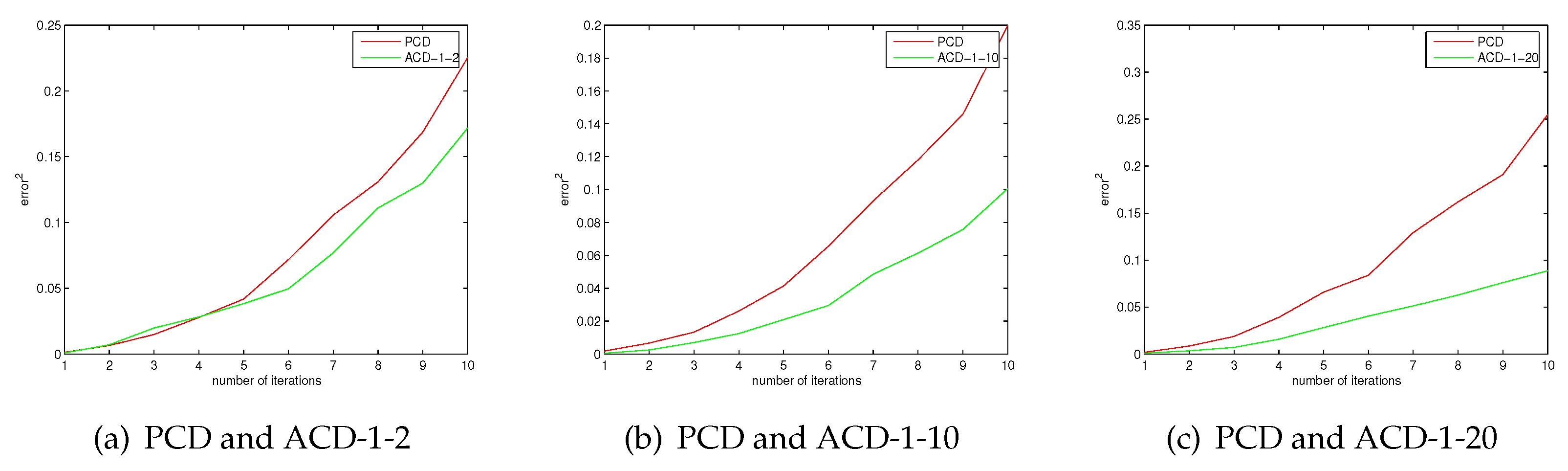
It is known that CD-k is closer to the log-likelihood gradient as k is larger. In the case of the same number of iterations, ACD-1-k and CD-k have same computational complexity. We give the results of 10 iterations. More iterations can be considered, which will require more training time. However, 10 iterations is enough to illustrate the approximation error of these algorithms. Figure 1 shows the approximation error of ACD and CD. The results show that the approximation error of ACD is smaller than that of CD. We can see that ACD is a better approximation of the log-gradient than CD from Figure 1, the experimental results are consistent with the conclusion of Theorem 5. In the case of the same number of iterations, the computational complexity of CD-20 is greater than ACD-1-10; however, Figure 1 shows that the approximation error of ACD-1-10 is smaller than CD-20, even if ACD-1-2 has a smaller approximation error than CD-20. One may find that the approximation error is very small as the number of iterations is small. The reason is that all algorithms are tested under exactly the same conditions. The initialized values of the parameters are the same. Figure 2 shows the approximation errors of ACD and PCD. There are similar experiment results about PCD and ACD. The results show that ACD has smaller approximation errors than PCD.

Figure 1. The approximation errors of average contrastive divergence (ACD) and CD.

Figure 1. The approximation errors of average contrastive divergence (ACD) and CD.

Figure 2. The approximation errors of ACD and persistent contrastive divergence (PCD).

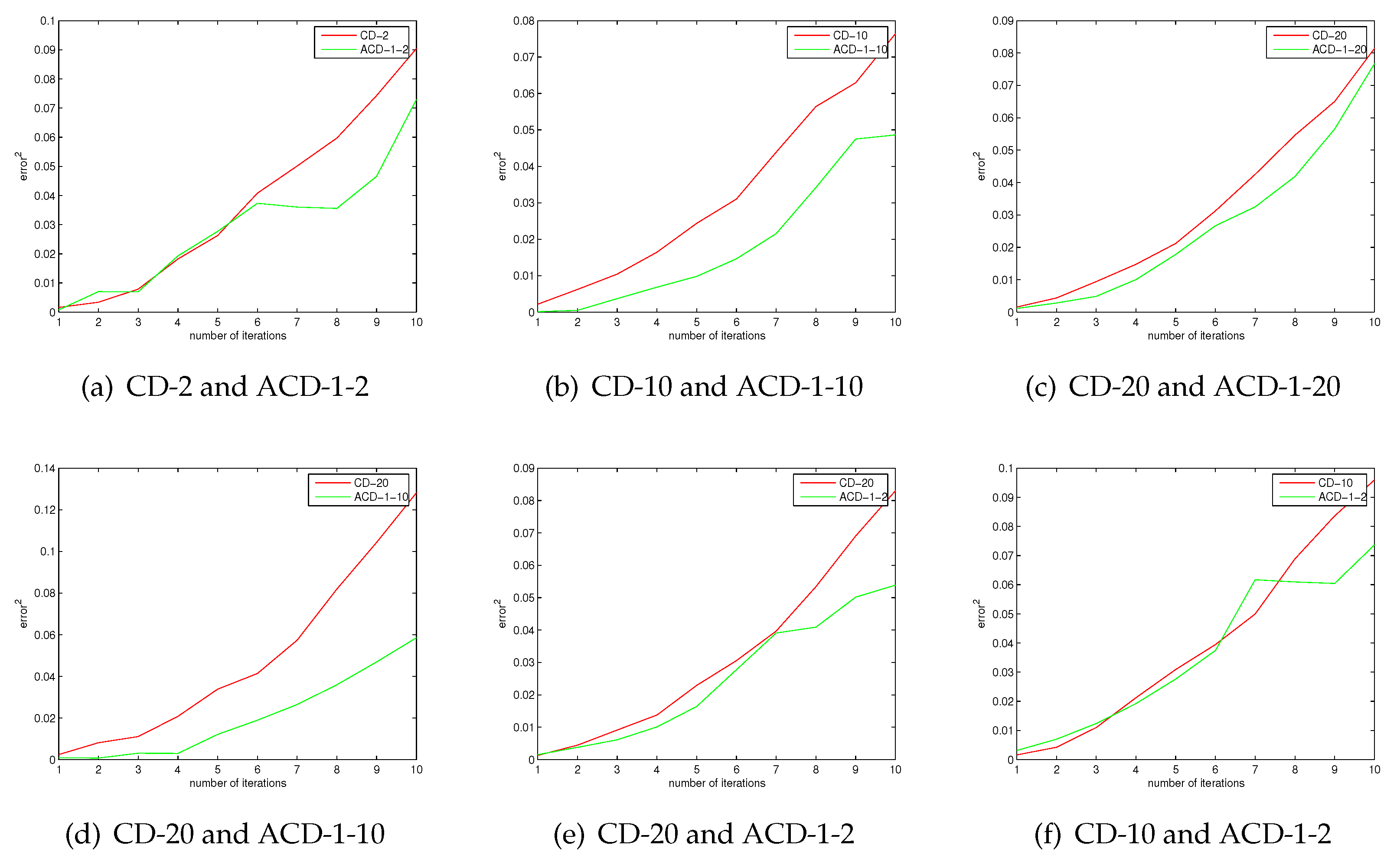
Figure 2. The approximation errors of ACD and persistent contrastive divergence (PCD).

4.2. The MNIST Task

The dataset is the MNIST dataset of handwritten digital images [20]. The images are 28 by 28 pixels, and the dataset consists of 60,000 training cases and 10,000 test cases. We use the mini-batch strategy for learning by only using a small number of training cases for each gradient estimate. We used 100 training points in each mini-batch for most datasets. Following [14,18,21,22], we set the number of hidden units to 500 in our experiments. One of the evaluations is how well the learned RBM models the test data, i.e., log-likelihood. This is intractable for a regular size of RBMs, because the time complexity of that computation is exponential in the size of the smallest layer (visible and hidden). Salakhutdinov and Murray [23] showed that a Monte Carlo-based method, annealed importance sampling (AIS), can be used to efficiently estimate the normalization constant Z of RBMs [16,23,24,25,26]. We adopt AIS in our experiment, as well.

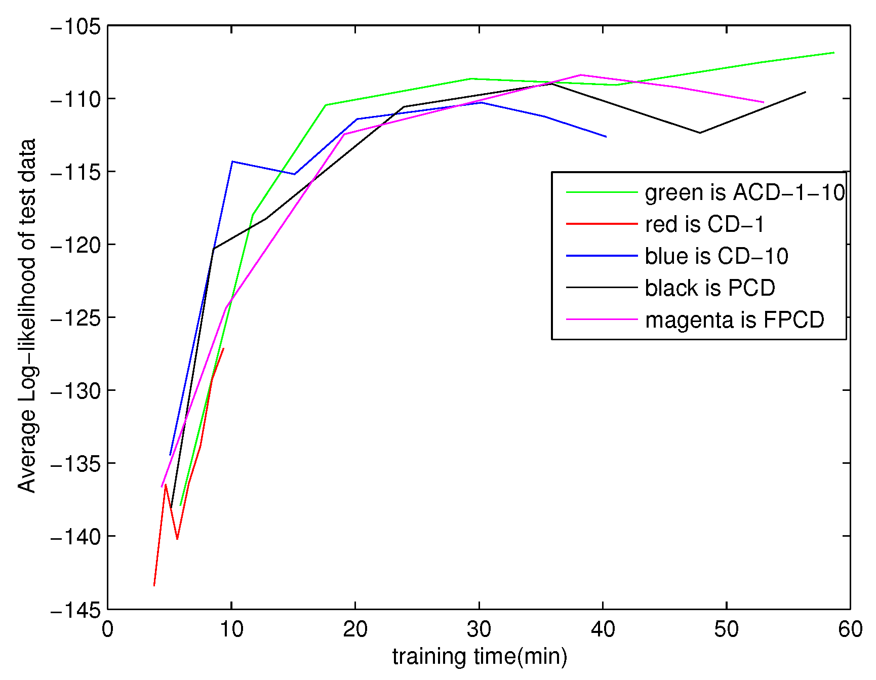
The CD algorithm and the PCD algorithm have become two popular methods for training RBMs. Tieliman and Hinton proposed an improved PCD algorithm called fast PCD (FPCD) [15]. The FPCD algorithm attempts to improve upon PCD’s mixing properties by introducing a group of additional parameters called fast parameters that are only used for sampling. FPCD tries to get out of any single mode of the distribution by these fast learning parameters and achieves better results in approximating the RBMs’ gradient. We consider the CD-1 algorithm, the CD-10 algorithm, the PCD algorithm, the FPCD algorithm and the ACD-1-10 algorithm for the MNIST task. The results on the MNIST task are shown in Figure 3. Figure 3 gives the average log-likelihood on the test dataset. The lower the average log-likelihood on the test dataset is, the more the contribution of the approximation of the gradient is. It is clear that ACD-1-10 outperforms CD-1, CD-10, PCD and FPCD. In the initial stages of training, the result of ACD-1-10 is close to the other algorithms. ACD-1-10 has better performance than the other algorithms with the increase of training time.

Figure 3. Modeling MNIST data with 500 hidden units (approximation log-likelihood).

Figure 3. Modeling MNIST data with 500 hidden units (approximation log-likelihood).

5. Conclusions

In this paper, we studied the CD algorithm and proposed a new algorithm for training RBMs. We have given the bias between the CD algorithm and the log-likelihood gradient method. We generalized the conclusions of Bengio and Delalleau; we can obtain their conclusions from our theorems; hence, we gave new proofs and interpretations of their results. Meanwhile, we proposed the ACD algorithm for training RBMs. We gave the bias between the ACD algorithm and the log-likelihood gradient. We experimentally studied the ACD algorithm; the results show that the ACD algorithm is a better approximation of the log-likelihood gradient method than the standard CD and PCD. The ACD algorithm outperforms the other learning algorithms.

Much work still remains. In order to evaluate the learned RBMs, we considered the log-likelihood. We used annealed importance sampling (AIS) to calculate the log-likelihood, but its reliability has not been researched extensively. An effective algorithm is needed. Furthermore, the amount of training time used in our experiments is insufficient to find the asymptotic performance. In Figure 3, one can see, for example, that ACD clearly profits from more training time. It is future work to find out what its performance would be with more training time.

References

- Hinton, G.E. Training products of experts by minimizing Contrastive Divergence. Neural Comput. 2002, 14, 1771–1800. [Google Scholar] [CrossRef] [PubMed]
- Hinton, G.E. Learning multiple layers of representation. Trends Cognit. Sci. 2007, 11, 428–434. [Google Scholar] [CrossRef] [PubMed]
- Hinton, G.E.; Osindero, S.; Teh, Y.W. A Fast Learning Algorithm for Deep Belief Nets. Neural Comput. 2006, 18, 1527–1554. [Google Scholar] [CrossRef] [PubMed]
- Feng, F.; Li, R.; Wang, X. Deep correspondence restricted Boltzmann machine for cross-modalretrieval. Neurocomputing 2015, 154, 50–60. [Google Scholar] [CrossRef]
- Bengio, Y.; Lamblin, P.; Popovici, D.; Larochelle, H. Greedy layewise training of deep networks. In Advances in Neural Information Processing (NIPS19); Schoőlkopf, B., Platt, J., Hoffman, T., Eds.; MIT Press: Cambridge, MA, USA, 2007; pp. 153–160. [Google Scholar]
- Bengio, Y.; Delalleau, O. Justifying and generalizing contrastive divergence. Neural Comput. 2009, 21, 1601–1621. [Google Scholar] [CrossRef] [PubMed]
- Fischer, A.; Igel, C. An Introduction to Restricted Boltzmann Machines; CIARP2012; Springer: Berlin, Germany, 2012; pp. 14–36. [Google Scholar]
- Akaho, S.; Takabatake, K. Information Geometry of Contrastive Divergence; ITSL2008; CSREA Press: Las Vegas, NV, USA, 2008; pp. 3–9. [Google Scholar]
- Sutskever, I.; Tieleman, T. On the convergence properties of Contrastive Divergence. J. Mach. Learn. Res. Proc. Track 2010, 9, 789–795. [Google Scholar]
- Yuille, A. The convergence of contrastive divergence. In Advances in Neural Processing Systems, NIPS17; Saul, L., Weiss, Y., Bottou, L., Eds.; MIT Press: Cambridge, MA, USA, 2005; pp. 1593–1600. [Google Scholar]
- Carreira-Perpinán, M.Á.; Hinton, G.E. On contrastive divergence learning. In Proceedings of the 10th International Workshop on Artificial Intelligence and Statistics (AISTATS), The Society for Artificial Intelligence and Statistics, The Savannah Hotel, Barbados, 6–8 January 2005; pp. 59–66.
- Ma, X.; Wang, X. Convergence analysis of contrastive divergence algorithm based on gradient method with errors. Math. Probl. Eng. 2015, 2015, 350102. [Google Scholar] [CrossRef]
- Fischer, A.; Igel, C. Bounding the bias of contrastive divergence learning. Neural Comput. 2011, 23, 664–673. [Google Scholar] [CrossRef] [PubMed]
- Tieleman, T. Training restricted Boltzmann machines using approximations to the likelihood gradient. In Proceedings of the International Conference on Machine learning (ICML), Helsinki, Finland, 5–9 July 2008; Cohen, W.W., McCallum, A., Roweis, S.T., Eds.; ACM: New York, NY, USA, 2008; pp. 1064–1071. [Google Scholar]
- Tieleman, T.; Hinton, G.E. Using fast weights to improve persistent contrastive divergence. In Proceedings of the International Conference on Machine Learning (ICML), Montreal, QC, Canada, 14–18 June 2009; Pohoreckyj Danyluk, A., Bottou, L., Littman, M.L., Eds.; ACM: New York, NY, USA, 2009; pp. 1033–1040. [Google Scholar]
- Cho, K.; Raiko, T.; Ilin, A. Parallel tempering is efficient for learning restricted Boltzmann machines. In Proceedings of the International Joint Conference on Neural Networks (IJCNN), Barcelona, Spain, 18–23 July 2010; IEEE Press: âĂŐPiscataway, NJ, USA, 2010; pp. 3246–3253. [Google Scholar]
- Cho, K.; Raiko, T.; Ilin, A. Enhanced Gradient for Training Restricted Boltzmann Machines. Neural Comput. 2013, 25, 805–831. [Google Scholar] [CrossRef] [PubMed]
- Desjardins, U.; Courville, A.; Bengio, Y.; Vincent, P.; Delalleau, O. Tempered Markov Chain Monte Carlo for Training of Restricted Boltzmann Machines; AISTATS: Sardinia, Italy, 2010; pp. 145–152. [Google Scholar]
- Younes, L. Parametric inference for imperfectly observed gibbsian fields. Probab.Theory Relat. Fields 1989, 82, 625–645. [Google Scholar] [CrossRef]
- LeCun, Y.; Cortes, C.; Burges, C. The MNIST database of handwritten digits. Available online: http://yann.lecun.com/exdb/mnist/ (accessed on 2 November 2013).
- Xu, J.; Li, H.; Zhou, S. Improving mixing rate with tempered transition for learning restricted Boltzmann machines. Neurcomputing 2014, 139, 328–335. [Google Scholar] [CrossRef]
- Fischer, A.; Igel, C. Training restricted Boltzmann machines: An introduction. Pattern Recognit. 2014, 47, 25–39. [Google Scholar] [CrossRef]
- Salakhutdinov, R.; Murray, I. On the quantitative analysis of deep belief networks. In Proceedings of the International Conference on Machine Learning, Helsinki, Finland, 5–9 July 2008; pp. 872–879.
- Salakhutdinov, R.; Larochelle, H. Efficient Learning of Deep Boltzmann Machines; AISTATS: Sardinia, Italy, 2010; pp. 693–670. [Google Scholar]
- Salakhutdinov, R. Learning Deep Boltzmann Machines Using Adaptive MCMC; ICML2010, Omnipress: Madison, WI, USA, 2010; pp. 943–950. [Google Scholar]
- Salakhutdinov, R.; Hinton, G.E. An efficient learning procedure for deep Boltzmann machines. Neural Comput. 2012, 24, 1967–2006. [Google Scholar] [CrossRef] [PubMed]
© 2016 by the authors; licensee MDPI, Basel, Switzerland. This article is an open access article distributed under the terms and conditions of the Creative Commons by Attribution (CC-BY) license (http://creativecommons.org/licenses/by/4.0/).
Share and Cite
MDPI and ACS Style
Ma, X.; Wang, X. Average Contrastive Divergence for Training Restricted Boltzmann Machines. Entropy 2016, 18, 35. https://doi.org/10.3390/e18010035
AMA Style
Ma X, Wang X. Average Contrastive Divergence for Training Restricted Boltzmann Machines. Entropy. 2016; 18(1):35. https://doi.org/10.3390/e18010035
Chicago/Turabian StyleMa, Xuesi, and Xiaojie Wang. 2016. "Average Contrastive Divergence for Training Restricted Boltzmann Machines" Entropy 18, no. 1: 35. https://doi.org/10.3390/e18010035
Note that from the first issue of 2016, this journal uses article numbers instead of page numbers. See further details here.