A Lattice Gas Automata Model for the Coupled Heat Transfer and Chemical Reaction of Gas Flow Around and Through a Porous Circular Cylinder

Abstract

Coupled heat transfer and chemical reaction of fluid flow in complex boundaries are explored by introducing two additional properties, i.e. particle type and energy state into the Lattice gas automata (LGA) Frisch–Hasslacher–Pomeau (FHP-II) model. A mix-redistribute of energy and type of particles is also applied on top of collision rules to ensure randomness while maintaining the conservation of mass, momentum and energy. Simulations of heat transfer and heterogeneous reaction of gas flow passing a circular porous cylinder in a channel are presented. The effects of porosity of cylinder, gas inlet velocity, and reaction probability on the reaction process are further analyzed with respect to the characteristics of solid morphology, product concentration, and temperature profile. Numerical results indicate that the reaction rate increases with increasing reaction probability as well as gas inlet velocity. Cylinders with a higher value of porosity and more homogeneous structure also react with gas particles faster. These results agree well with the basic theories of gas–solid reactions, indicating the present model provides a method for describing gas–solid reactions in complex boundaries at mesoscopic level.

1. Introduction

The simulation of heat transfer and chemical reaction of fluid flow in porous media is of considerable importance in many practical applications such as combustion chambers, heat exchangers, food processing, catalytic reactors, refrigeration, air cooling and thermal energy storage devices. Simulation results can be found for porous catalyst particles, packed catalyst beds, and arranged pipes. Among these studies, methods based on conventional partial differential equations such as volume-averaging theory [1] and Darcy models [2,3,4], or discrete methods, e.g., lattice Boltzmann methods (LBM) [5,6,7,8] have been the major approaches. However, to the best of our knowledge, the porous media reported in the literature are relatively simple and usually consist of regular arranged solid cylinders. Few studies have been carried out to investigate the characteristics of heat transfer coupling by chemical reaction in porous media. Additionally, the conventional methods based on nonlinear partial differential equations (PDEs) also suffer difficulties such as truncation error and high sensitivity to boundary conditions, making it difficult to describe the detailed structure of porous media or simulate complex processes in porous media.

Lattice gas automata (LGA) is a mesoscopic simulation method from the viewpoint that fluids consist of a large number of particles that “live” on regular lattices with interactions conserving mass and momentum [9]. It is a “bottom-up” and “equation-free” method capturing both macroscopic and mesoscopic characteristics of complex/multi-scale systems, quite distinctive from molecular dynamics (MD), kinetic theory of gases and other methods based on the discretization of partial differential equations. Although LGA suffers drawbacks like statistical noise, the lake of Galilean invariance and velocity-dependent pressure, LGA preserves the particle nature and numerical stability compared with lattice Boltzmann methods [10]. More detailed microscopic interaction among particles or between particles and walls can be obtained when using LGA. Thus, various investigations on flow past obstacles or reaction using lattice gas automata have been carried out, such as flow over cylinders or plat plate [11,12,13], reaction and diffusion systems [14,15,16], first order reactions [17], motivation phenomena of atom and molecule [18,19], kinetically and thermodynamically controlled reactions [20,21,22], and Lindemann theory [23,24]. However, investigations on flow, heat transfer and chemical reaction around a porous cylinder using LGA were rarely reported.

Therefore, in this paper, we intend to explore the application of a LGA method to the heat transfer and chemical reaction of fluid flow around and through a porous circular cylinder in a channel. An algorithm based on the Frisch–Hasslacher–Pomeau (FHP-II) LGA model was developed to deal with the coupled heat transfer and chemical reaction. Quartet structure generation set (QSGS) was used to construct the porous circular cylinder. The influences of porous structure, i.e. porosity, pore size and homogeneity, as well as that of reaction probability and flow velocity were further discussed.

2. Simulation Method

2.1. Lattice Gas Automata Model for Heat Transfer and Chemical Reaction

In FHP-II, particles interact with each other according to a number of pre-defined collision and propagation rules detailed by Frish et al. [25], as shown in Figure 1. Based on these simple rules, LGA is capable of displaying complex fluid flow behavior, and consequently, it can be used as a simulation tool for describing physical phenomena. The mass and momentum conservation can be written as below, respectively,

$${\displaystyle \sum _i{n}_i(t+1,r+c_i)}={\displaystyle \sum _i{n}_i(t,r)}$$

(1)

$${\displaystyle \sum _i{c}_i{n}_i(t+1,r+c_i)}={\displaystyle \sum _i{c}_i{n}_i(t,r)}$$

(2)

where $n_i(t,r)$ is the occupation state of the cell in i-th direction at time $t$ and place $r$ if the cell is empty, its value is 0, otherwise, its value is 1. $c_i$ is the lattice velocity in i-th direction, and

$$c_i\text{=}\{\begin{array}{l}\left(\text{cos}\frac{\pi }{\text{3}}i,\sin \frac{\pi }{\text{3}}i\right),i=1,\dots ,6\\ 0,i=0\end{array}$$

Figure 1. Evolution process of FHP-II, where arrows denote moving particles and points represent static particles: (a) node at (t, r); (b) initialization; (c) after collision; and (d) after propagation.

Figure 1. Evolution process of FHP-II, where arrows denote moving particles and points represent static particles: (a) node at (t, r); (b) initialization; (c) after collision; and (d) after propagation.

In the conventional LGA model, particles in the system are of same mass (assumed as 1) and velocity scale (assumed as |$c_i$| = 1), in other words, they are indistinguishable. In order to describe problems involving heat transfer and chemical reactions, the particles should be distinguishable on temperature and substance type. In current model, every particle is at either of the two energy states [26] $e_i$, i.e., 0 or 1, which represent low (minimum) and high (maximum) temperatures, respectively. Particularly, if the cell is empty, $e_i$ is fixed as 0. Particles are also marked by finite kinds of substance types $s_i$, and in this paper, $s_i$ is equal to 0 or 1, representing reactant and product, respectively. Besides mass and momentum, extra conservations are also taken into account with respect to energy state and substance type, given as

$${\displaystyle \sum _i{n}_i^{\alpha ,\beta }(t+1,r)}={\displaystyle \sum _i{n}_i^{\alpha ,\beta }(t,r)}$$

(3)

where α and β are the substance type and energy state of the cell in i-th direction, respectively. To ensure the conservation of the number of particles with different energy states and substance types at each node during the collision step of FHP-II model, the substance type and energy state need to follow Equations (4) and (5), respectively, known as component conservations

$${\displaystyle \sum _i{s}_i^{\alpha }(t+1,r)}={\displaystyle \sum _i{s}_i^{\alpha }(t,r)},\alpha =1or0$$

(4)

$${\displaystyle \sum _i{e}_i^{\beta }(t+1,r)}={\displaystyle \sum _i{e}_i^{\beta }(t,r)},\beta =1or0$$

(5)

Afterwards, the energy states and substance types of each node are mixed and re-distributed. In fact, the energy states and substance types will be arbitrarily attached to the particles at the node after collision. The overall conservations of mass and momentum will still follow Equations (1) and (2). However, for the propagation process, the particle will move with energy state and substance type, which is described as Equation (6). The evolution process of this model is illustrated in Figure 2.

$$n_i^{s_i(t+1,r+c_i),e_i(t+1,r+c_i)}(t+1,r+c_i)=n_i^{s_i(t,r),e_i(t,r)}(t,r)$$

(6)

Figure 2. Evolution process of present model, where red represents particles with high energy state, black represents particles with low energy state, and double arrows mean product particles and single arrows denote reactant particles: (a) initialization; (b) after collision; and (c) after propagation.

Figure 2. Evolution process of present model, where red represents particles with high energy state, black represents particles with low energy state, and double arrows mean product particles and single arrows denote reactant particles: (a) initialization; (b) after collision; and (c) after propagation.

In FHP-II, the density and momentum are defined as

$$\rho (t,r)={\displaystyle \sum _{i=0}^6{n}_i(t,r)}$$

(7)

$$\rho u={\displaystyle \sum _{i=0}^6{c}_i{n}_i(t,r)}$$

(8)

The temperature and product concentration at a node are described as the proportion of particles with high energy state (β = 1) and the proportion of product particles (α = 1), respectively, as the following dimensionless forms:

$$T=\frac{{\displaystyle \sum _i{n}_i^{\alpha ,1}(t,r)}}{{\displaystyle \sum _{i,\beta }{n}_i^{\alpha ,\beta }(t,r)}}$$

(9)

$$C=\frac{{\displaystyle \sum _i{n}_i^{1,\beta }(t,r)}}{{\displaystyle \sum _{i,\alpha }{n}_i^{\alpha ,\beta }(t,r)}}$$

(10)

2.2. Chemical Reaction Scheme

The scheme of chemical reaction is based on the algorithm proposed by Bresolin and Oliveira [27] to simulate unimolecular and bimolecular reactions. For first-order reactions considering unimolecular collision, the rate constant, $k$, is described as

$$k={\displaystyle {\int }_0^{\infty }v(E)P(E)dE}$$

(11)

where $v(E)$ is the frequency of collisions with energy $E$ above the minimum energy $E^{*}$, $P(E)$ is the energy distribution of the molecules, which is given by the Maxwell–Boltzmann distribution, and for a molecule with n classic energy states, the fraction of molecules with energy states $E_1$,$E_2$,…,$E_n$ can be written as

$$P(E_1,E_2,\dots E_n)=\frac{e^{\frac{-(E_1+E_2+\dots E_n)}{RT}}}{RT}=\frac{e^{\frac{-E}{RT}}}{RT}$$

(12)

Integrating Equation (12) over all energy values yields:

$$P(E)={\left(\frac{E}{RT}\right)}^{n-1}\frac{e^{\frac{-E}{RT}}}{(n-1)!RT}$$

(13)

According to Rice–Ramsperger–Kassel (RRK) model [28,29,30], the frequency of collisions $v(E)$ is suggested to be the formula as follows:

$$\{\begin{array}{l}\overline{v(E)}=0ifE<E^{*}\\ \overline{v(E)}=C(1-\frac{E^{*}}{E}{)}^{n-1}ifE\ge E^{*}\end{array}$$

(14)

where C is a constant. For the simulation of chemical reaction in LGA, the collisions between molecules can be interpreted as taking place among particles at a node.

In this paper, each reactant particle propagates with an associated probability r deciding it reacts and converts to a product particle or not, generally described as the probability of effective collision. This probability is determined by a probability distribution function and a threshold for reaction. Herein, for simplification, the standard Gaussian distribution was used as the probability distribution function instead of Maxwell–Boltzmann distribution, a threshold K^* was used instead of E^* to decide the critical energy state of a reactant particle. During the collision step of LGA, a random number K following the probability distribution function is generated and compared to K^*; if K > K^*, the reaction is consider to be able to take place, otherwise, no reaction occurs.

Moreover, the frequency of collisions in LGA is supposed to be 1.0 per iteration when K > K^*, otherwise its value is 0, similar to Equation (14). Thus, the specific reaction constant equals to the integration of energy distribution function above K^* according to Equation (11). Therefore, reaction probability r is equal to the proportion of the particles with energy above K^*, as well as the specific reaction constant. As shown in Figure 3, the curve represents the probability distribution function (PDF), and K^* is a threshold for reaction, the shaded area (beyond K^*) represents the frequency of collisions of hot populations, i.e., reaction probability r. For a given K^*, reaction probability is obtained, and vice versa. In this work, K^* was determined by a given reaction probability from the inverse of normal distribution [31]. The applications of the chemical reaction scheme will be further discussed.

Figure 3. Standard Gaussian distribution function for determining the probability of chemical reaction.

Figure 3. Standard Gaussian distribution function for determining the probability of chemical reaction.

3. Results and Discussion

3.1. Validation of the Chemical Reaction Scheme

The chemical reaction scheme was applied to irreversible first-order reaction $A\to B$ and reversible first-order reaction $A\rightleftharpoons B$, such as nuclear decay and transformation of isomers. The reactions take place in a square enclosure with area 200 × 200 (lattice units). Every site was initially filled with six A-type particles and bounce-back type boundary condition was employed to all walls, where the momentum of particle is directly reversed while the substance state keeps unchanged during the collision process. Additionally, no heat transfer was taken into consideration in these two cases.

Molecules collide and react at random. Nevertheless, the time evolution of macroscopic amounts or concentrations of molecules is usually quite reproducible due to the reproducibility of experimental conditions. Such laws are called deterministic. More detailed introduction can be found in reference [32]. 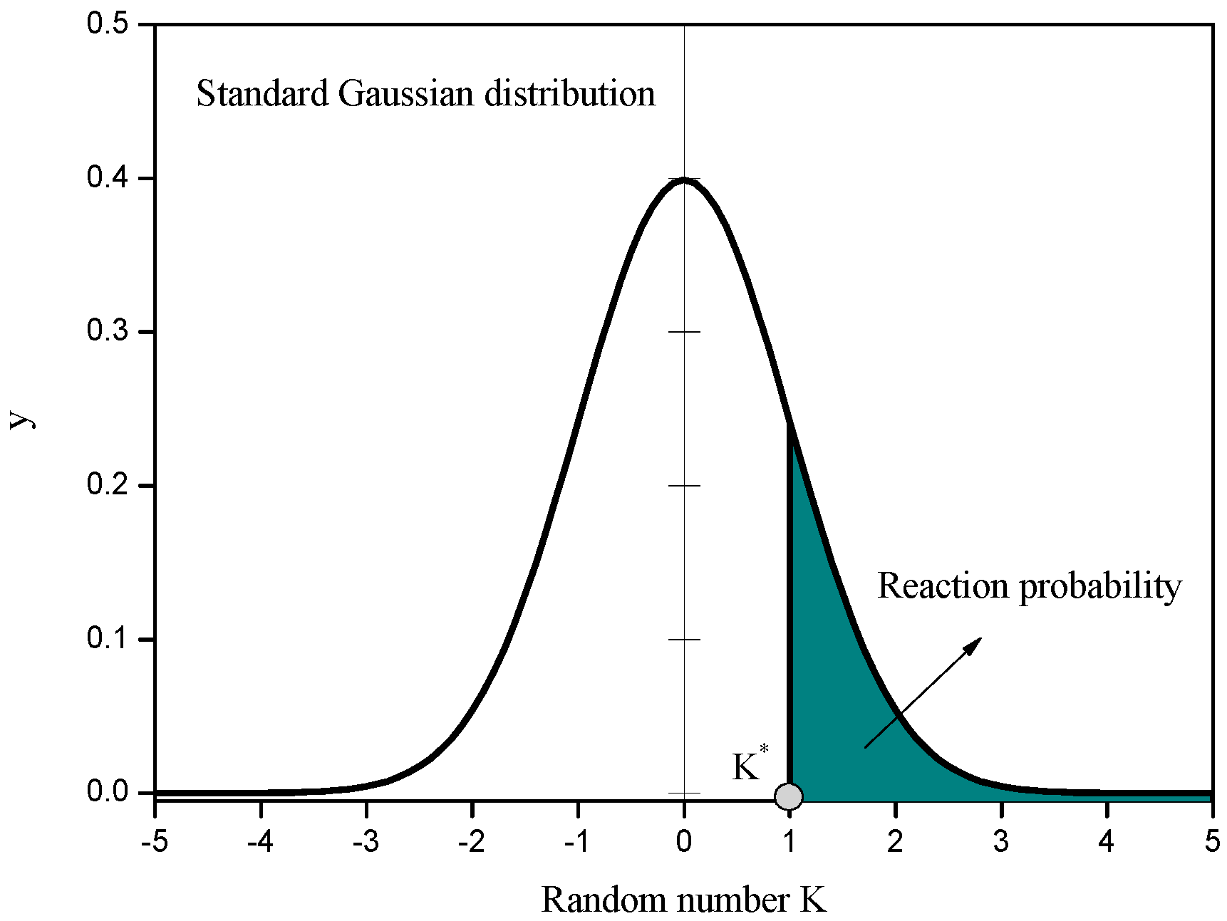For reaction $A\to B$, the deterministic half-life period can be obtained by $t_{1/2}=\ln 2/R$, where r represents the probability of one A-type particle changes to one B-type particle at each time, while the half-life period means the iterations needed for reducing the number of A-type particle by half during the simulation process. The reaction probability, r, from A to B was set to be 0.03, 0.04 and 0.05, and K^* was determined as 1.88, 1.75 and 1.65, respectively. 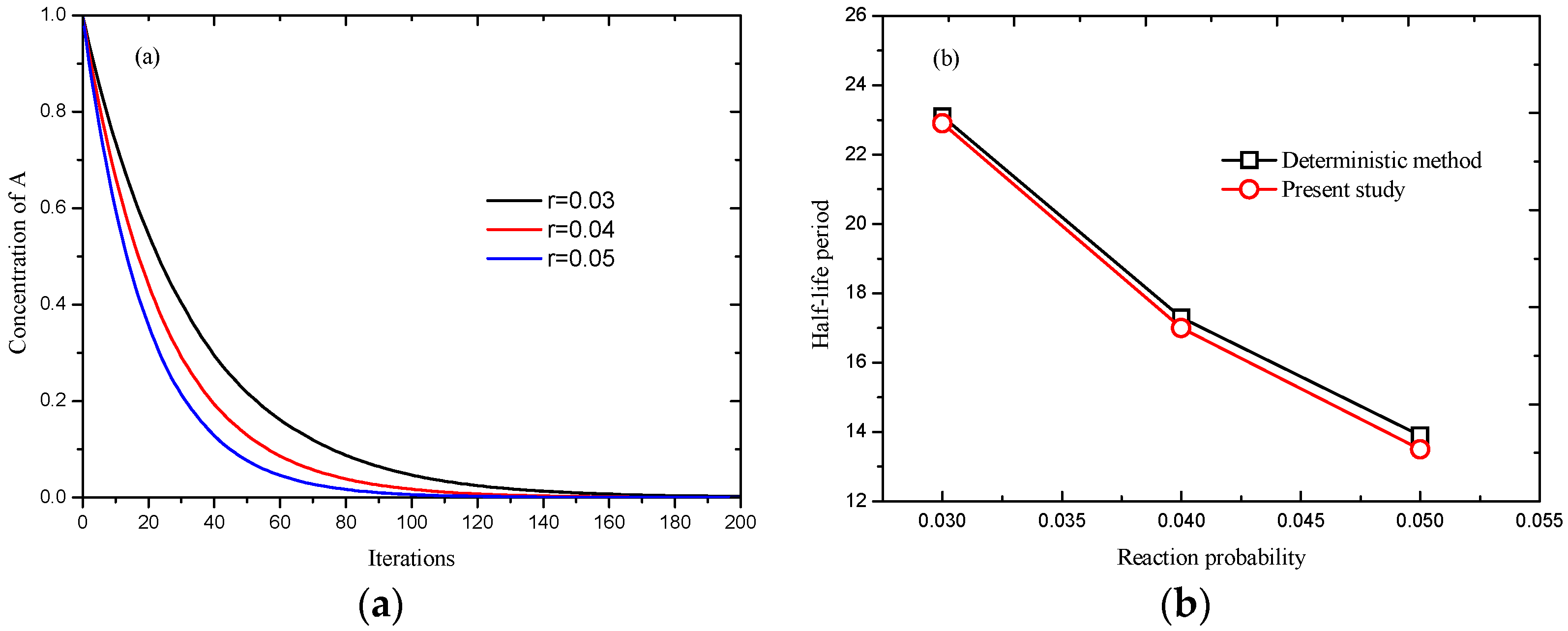During the collision process, a normal distributed random number was generated to compare with K^* to decide to react or not. As shown in Figure 4, it can be observed that the concentration of particle A, obtained by Equation (10), decreases with increasing reaction time, and the reaction rate, i.e., the slope of curve in Figure 4a, increases as reaction probability increases. Figure 4b shows reasonable agreement has been achieved between deterministic method and present simulation. Additionally, for a system with 100 × 100, and reduction probability r = 0.001, the deterministic half-life period is 693.1 iterations, Seybold et al. [17] reported 688.3 ± 9.7 iterations, and 691 iterations using present model, which also indicates the feasibility of present model in reaction systems.

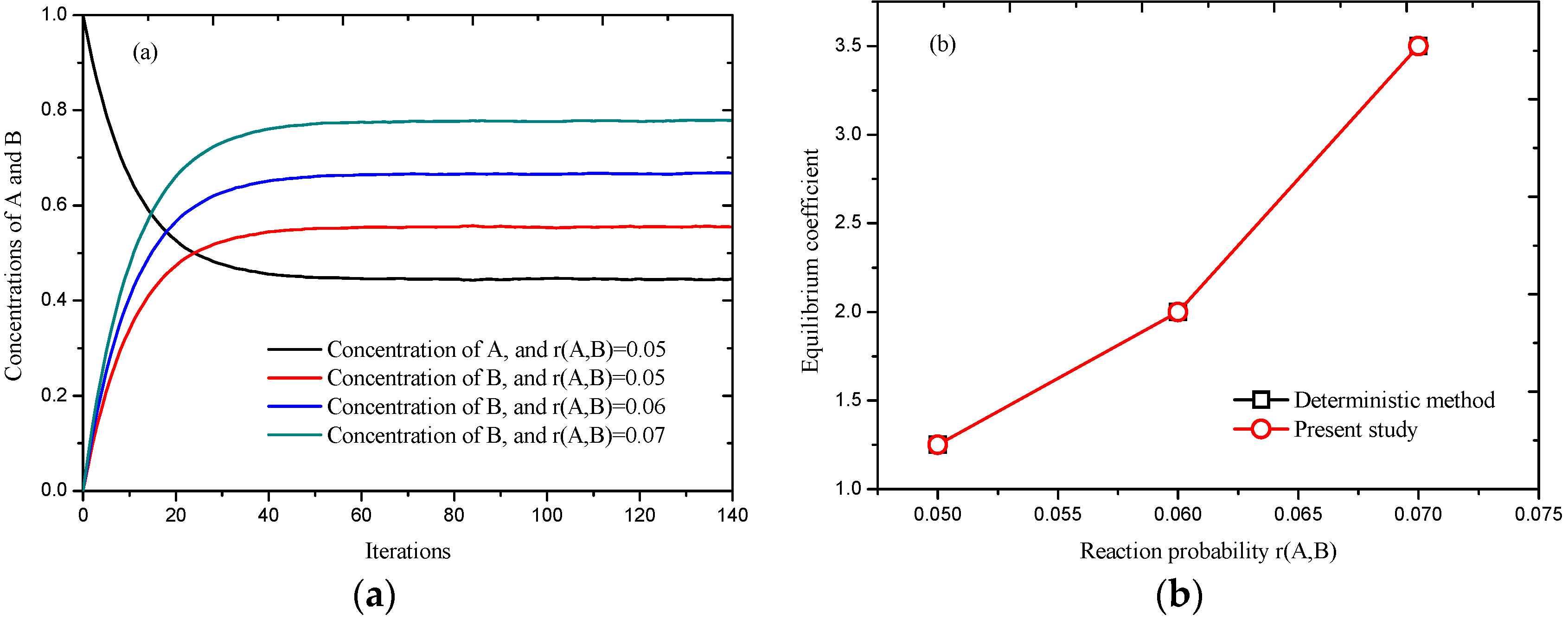
While $A\underset{k_2}{\overset{k_1}{\rightleftharpoons }}B$ is an equilibrium system, from the law of mass action, the deterministic equilibrium coefficient is defined as $K_{eq}=k_1/k_2=R(A,B)/R(B,A)$, and the equilibrium coefficient can be obtained by the ratio of the final concentration of B and A as $K_{eq}=[B]/[A]$ in a stochastic system, like simulations using lattice gas automata. The reaction probability from A to B was set as 0.05, 0.06, and 0.07, corresponding to the reaction probability from B to A 0.04, 0.03, and 0.02, and for reaction probability of 0.02 and 0.07, K^* is 2.05 and 1.48, respectively. Similar results are obtained compared to $A\to B$, as shown in Figure 5, however, Figure 5a presents a platform as time advances, meaning an equilibrium state has been reached. Figure 5b indicates that good agreement has been achieved between the stochastic method and deterministic method. The chemical reaction scheme will be further used for the simulations of gas–solid reaction described latter.

Figure 4. Simulation of $A\to B$, (a) processes at different reaction probabilities; and (b) comparison of results obtained by deterministic method and present model.

Figure 4. Simulation of $A\to B$, (a) processes at different reaction probabilities; and (b) comparison of results obtained by deterministic method and present model.

Figure 5. Simulation of $A\rightleftharpoons B$, (a) processes at different reaction probabilities; and (b) comparison of results obtained by deterministic method and present model.

Figure 5. Simulation of $A\rightleftharpoons B$, (a) processes at different reaction probabilities; and (b) comparison of results obtained by deterministic method and present model.

3.2. Heat Transfer and Reaction across a Porous Circular Cylinder

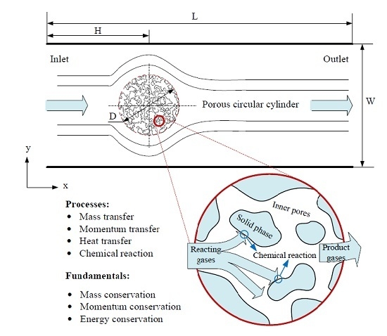
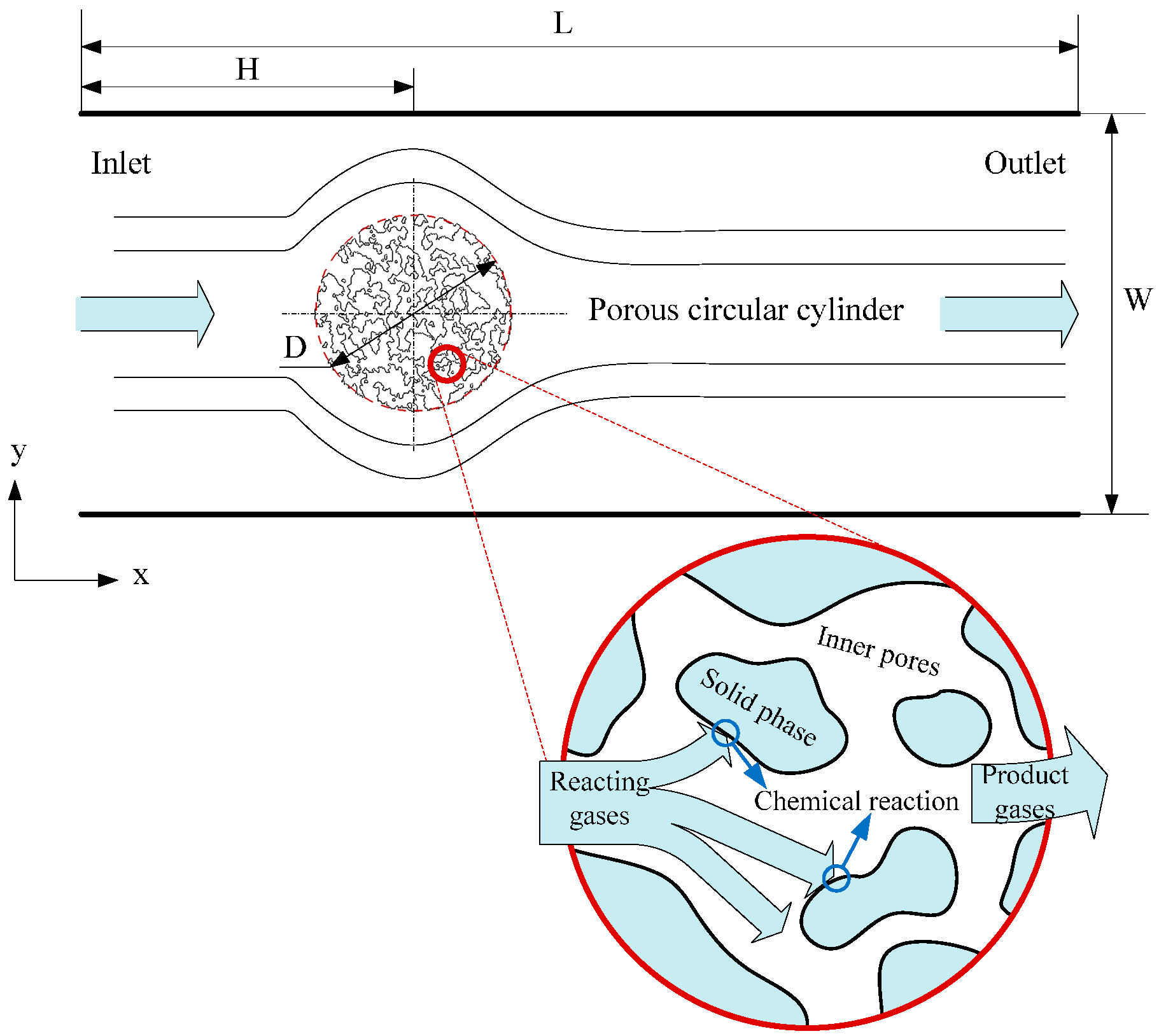
The characteristics of the flow and heat transfer over a solid circular cylinder in a square enclosure and a rectangular channel have been investigated by us using this model previously, showing reasonable feasibility and reliability of the application of this model to the problems of flow and heat transfer, details can be found in reference [33]. Herein, simulations of flow, heat transfer and reaction around and through a porous circular cylinder in a channel were carried out. The schematic diagram of the simulated system is shown as Figure 6, where a porous circular cylinder with diameter D = 1/4W is placed at the coordinates (x = 1/3L, y = 1/2W) of a channel with width W = 400 and length L = 1200 (lattice unit). Reactant gas entering from the inlet at a velocity u, flows around and through and react with the porous cylinder. The effects of porous structure, reaction probability and gas velocity at inlet on the characteristics of the system will be further discussed in detail.

The porous media investigated were generated by a comprehensive approach termed as quartet structure generation set (QSGS) [34,35], which has been demonstrated capable of generating morphological features close to many real porous media [34]. Following the steps illustrated by Wang et al. [23], a porous two-dimensional cylinder can be generated with a set of three construction parameters, including (i) growing phase (fluid) distribution probability, C_d, which decides initial number of fluid seeds in the system; (ii) directional growth probability of fluid, D_i, which is considered the same for all directions in this work; and (iii) fluid volume fraction P.

Figure 6. Schematic diagram of the processes happened in the circular cylinder with porous media structure.

Figure 6. Schematic diagram of the processes happened in the circular cylinder with porous media structure.

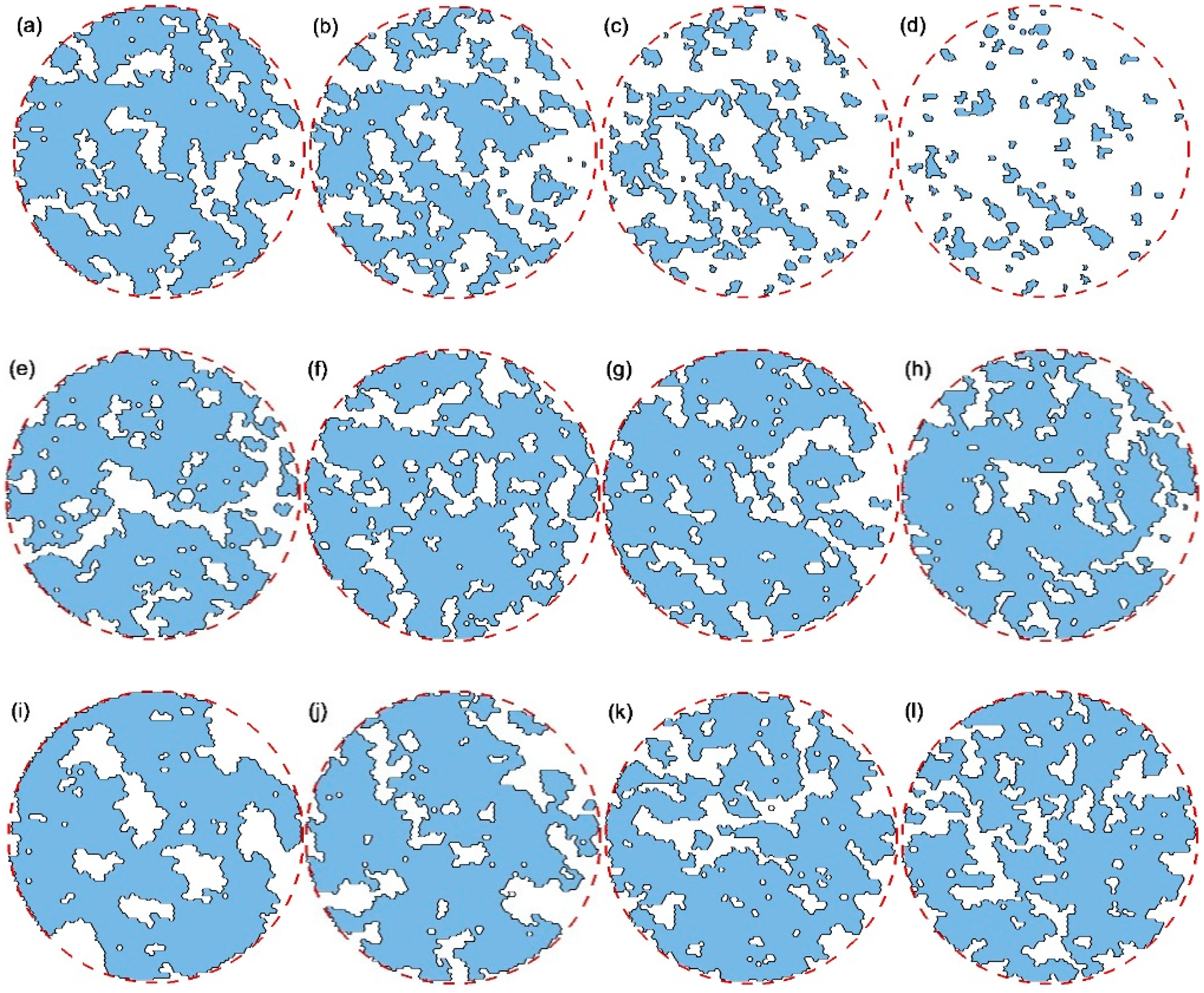
Figure 7 presents the inner morphology of the porous circular cylinders of diameter D = 100 (lattice unit) resulted from different combinations of construction parameters, where shaded area is solid phase and the rest to be pores. As can be seen in Figure 7a–d, the solid phase disappears homogenously with increasing porosity, leading to larger pore sizes; and for Figure 7e–h, more agglomeration of solid phase, i.e., less surface area and bigger pore size, appeared for larger directional growth probability; on the contrary, for Figure 7i–l, more homogenous structure as well as smaller pore size of porous media can be obtained as the distribution probability increases, as a result, more react-able surface area is generated. Porous cylinders of different porosity, pore size, and surface area could be obtained by adjusting the three parameters (C_d, D_i, P), for the purpose of comparison.

Figure 7. Porous cylinder generated with different construction parameter. (a–d) Effect of porosity on the morphology of cylinder, where C_d = 0.02, D_i = 0.2 and (a) P = 0.2, (b) P = 0.4, (c) P = 0.6, and (d) P = 0.8. (e–h) Effect of directional growth probability on the morphology of cylinder, where C_d = 0.02, P = 0.2 and (e) D_i = 0.05, (f) D_i = 0.15, (g) D_i = 0.25, and (h) D_i = 0.35. (i–l) Effect of distribution probability on the morphology of cylinder, where D_i = 0.2, P = 0.2 and (i) C_d = 0.005, (j) C_d = 0.015, (k) C_d = 0.025, and (l) C_d = 0.035.

Figure 7. Porous cylinder generated with different construction parameter. (a–d) Effect of porosity on the morphology of cylinder, where C_d = 0.02, D_i = 0.2 and (a) P = 0.2, (b) P = 0.4, (c) P = 0.6, and (d) P = 0.8. (e–h) Effect of directional growth probability on the morphology of cylinder, where C_d = 0.02, P = 0.2 and (e) D_i = 0.05, (f) D_i = 0.15, (g) D_i = 0.25, and (h) D_i = 0.35. (i–l) Effect of distribution probability on the morphology of cylinder, where D_i = 0.2, P = 0.2 and (i) C_d = 0.005, (j) C_d = 0.015, (k) C_d = 0.025, and (l) C_d = 0.035.

Table 1 lists the simulation cases with different parameter sets, with Cases 1 to 4 selected from Figure 7 to investigate the influence of the parameters of QSGS algorithm on the reaction process, Cases 1, 5 and 6 to study the effect of reaction probability, and Cases 1, 7 and 8 are used to investigate the inlet velocity.

Table 1. Parameter sets for simulation cases.

Case No.	Parameters of QSGS			r	u
	Cd	Di	P
1	0.02	0.2	0.2	0.1587	1.0
2	0.02	0.2	0.4	0.1587	1.0
3	0.035	0.2	0.2	0.1587	1.0
4	0.02	0.35	0.2	0.1587	1.0
5	0.02	0.2	0.2	0.0668	1.0
6	0.02	0.2	0.2	0.3085	1.0
7	0.02	0.2	0.2	0.1587	0.5
8	0.02	0.2	0.2	0.1587	0.8

Table 1. Parameter sets for simulation cases.

Case No.	Parameters of QSGS			r	u
	Cd	Di	P
1	0.02	0.2	0.2	0.1587	1.0
2	0.02	0.2	0.4	0.1587	1.0
3	0.035	0.2	0.2	0.1587	1.0
4	0.02	0.35	0.2	0.1587	1.0
5	0.02	0.2	0.2	0.0668	1.0
6	0.02	0.2	0.2	0.3085	1.0
7	0.02	0.2	0.2	0.1587	0.5
8	0.02	0.2	0.2	0.1587	0.8

A conceptual first order heterogeneous reaction between the reaction gas and the porous cylinder illustrated in Equation (10) is considered in this research, with A being the inlet reactant gas, B the porous solid material, and C as the product gas.

$$A(g)+B(s)\to C(g)$$

(15)

This reaction happens at the solid surface and is simply interpreted as one reactant gas particle reacting with one solid site and generating one product gas particle at mesoscopic level, where the (microscopic level) inner structures or properties of the gas particle or solid site are ignored. The conversion of solid phase B can be defined by the ratio of the number of reacted solid sites to the initial number of solid sites, and a formula as follows is defined

$$X=1-\frac{N_t}{N_0}$$

(16)

where N_t is the number of solid sites at time t, and N₀ is the initial number of solid sites. Thus, the reaction rate can be further obtained from the time derivative of Equation (11) as $dX/dt$.

Instead of heat generated during the reaction process, a simplified heat transfer case is considered, where solid sites are set as hot heat source with constant temperature (i.e. 1.0). Gaseous particles will be enhanced to high energy state at impact with solid surface. The gas particles initially entering the channel are of constant low temperature state as 0.

Bounce-back and adiabatic boundary conditions are applied to the channel walls except the outlet which is a free boundary where all particles are released. Solid sites are set as bounce-back boundaries, where gaseous particles will also decide to reaction with according to the chemical reaction scheme.

The simulation carried out in such an order that reaction is not considered in the first 2000 iterations to test the coupling of flow and heat transfer only, also to ensure that the reaction takes place at a stable flow field. Reaction is introduced thereafter to investigate its effect to the flow and heat transfer.

The statistical result of temperature, component concentration, and solid phase conversion are obtained from the simulation by space average. It is noted that the statistics level has impacts on the detail of macroscopic picture. This effect is, however, not discussed in this work. Instead, to ensure consistency, the space averaged results in every 2 × 2 grids are presented for all cases.

3.2.1. Effect of Inner Porous Structure

As discussed in the previous part, the inner porous structure will be influenced by the parameters of QSGS. In this section, the influence of inner structure on the behavior of flow, heat transfer and chemical reaction around and through the cylinder will be investigated. The inlet velocity is constant as 1.0 with a site density ρ = 1.0, and based on FHP-II model, Re = 158.2 using D as the characteristics parameter.

Figure 8 shows the temperature contours around and inside the porous cylinder before chemical reaction takes place at t = 2000 iterations. A large number of fluid particles are activated to high energy state when they flow over and in the porous circular cylinder, forming a high temperature zone at surrounding and inside the porous structure. As time elapses, the high temperature zone extends to the neighboring field gradually, and no clear eddies have developed behind the cylinder. The field of gas velocity also appeared to have impacts on the profile of temperature.

Figure 8. Temperature contour before reaction with different inner structures, t = 2000 iterations.

Figure 8. Temperature contour before reaction with different inner structures, t = 2000 iterations.

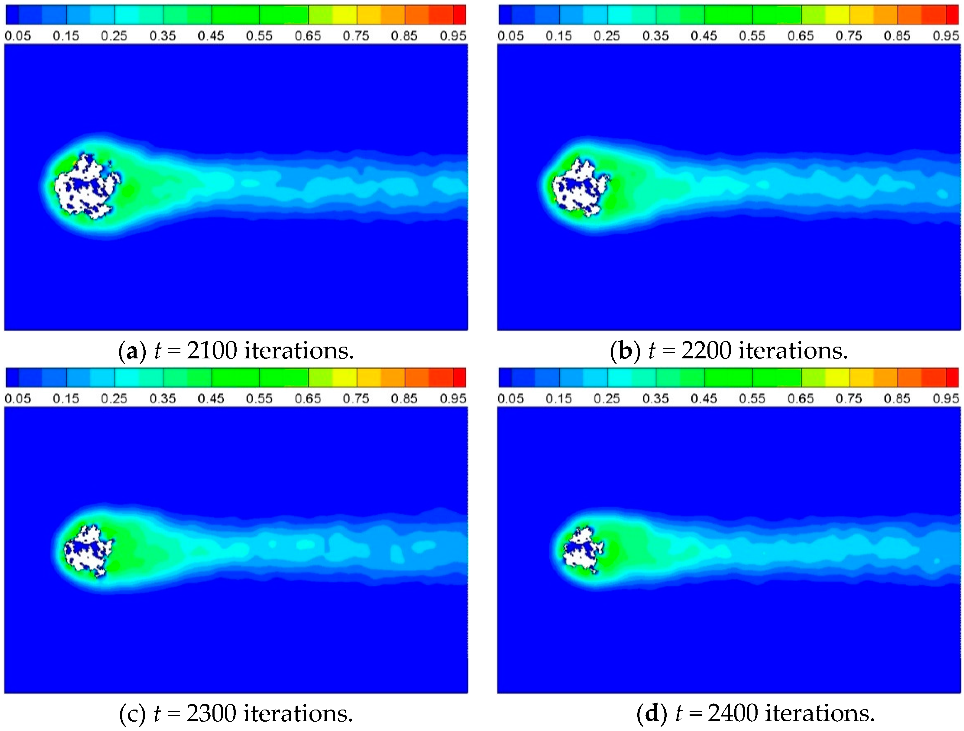
The heterogeneous reaction is started after 2000 iterations. A product zone is then formed as fluid particles flow over and through the porous cylinder and react with the solid sites according to the reaction scheme. Figure 9 shows the product concentration around the solid cylinder at different times for Case 4. The solid sites disappear gradually as time goes on. It can be observed that the product emerges mainly at some hot points, and distributes homogeneously around the cylinder at the beginning, and then diffuses off from the reaction interface to the surrounding. Figure 10 shows the corresponding temperature contour around the cylinder for Figure 9. The structure of cylinder changes with time, thus the heat transfer characteristics changes as a result.

Figure 9. Product concentration at different times for Case 4, where C_d = 0.02, D_i = 0.35, and P = 0.2.

Figure 9. Product concentration at different times for Case 4, where C_d = 0.02, D_i = 0.35, and P = 0.2.

Figure 10. Temperature contour at different times for Case 4, where C_d = 0.02, D_i = 0.35, and P = 0.2.

Figure 10. Temperature contour at different times for Case 4, where C_d = 0.02, D_i = 0.35, and P = 0.2.

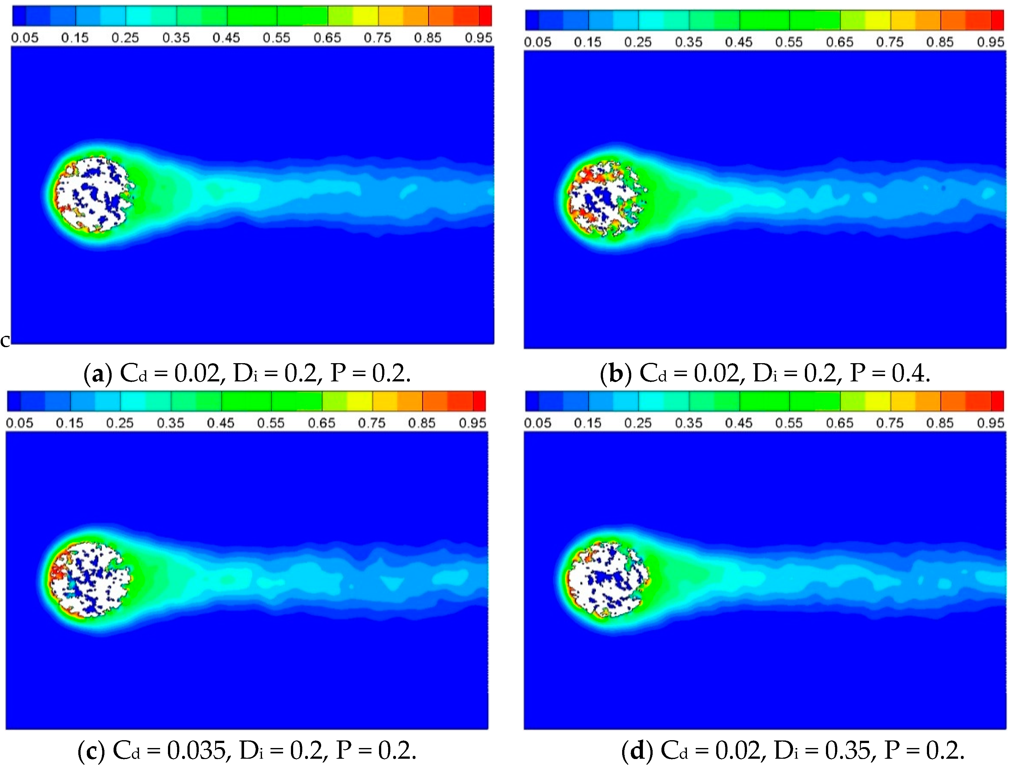
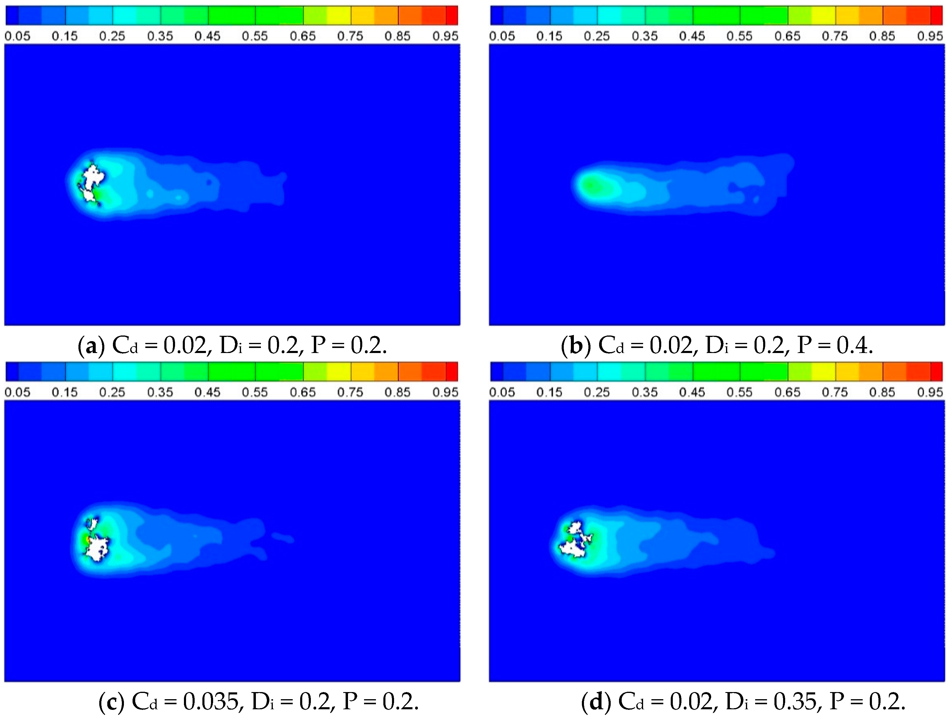
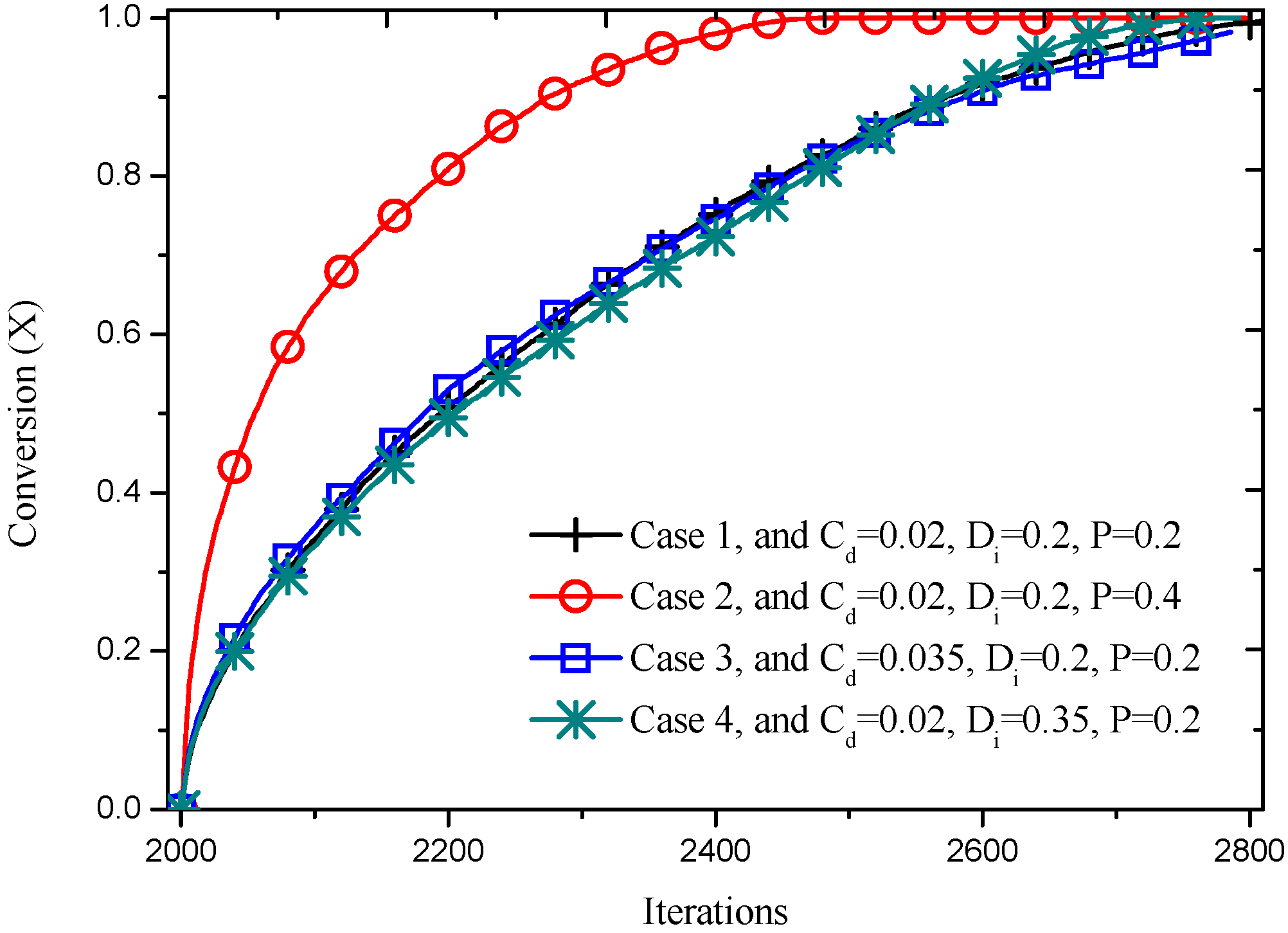
In order to compare the reaction characteristics of computational cases with porous inner structure, contours of product concentration are shown as Figure 11, for t = 2500. It can be observed that the solid cylinder has disappeared completely at t = 2500 for Case 2 which has higher porosity than the other three cases. Figure 12 shows the conversion of porous cylinders with different inner structure, as a function of time. It is also notable that solid conversion of higher porosity (Case 2) is faster. This is considered due to the less amount of solid phase, as well as the larger pore size, which facilitates the diffusion of reactant and product. The other three cases with same porosity of 0.2 proceed similarly, but it can still be noted that Case 3 with larger distribution probability progress faster than the other two cases for the former part of time, about 2500 iterations. This can be attributed to the higher homogeneity resulting from larger distribution probability, leading to a larger surface area (reacting sites) to mass ratio. However, this improvement on reaction speed is limited by the relatively smaller pore size slowing down the gas diffusion. Knowing this, it is understandable that Case 4, with larger solid agglomeration and bigger pore size due to higher value of directional growth probability, has the exact opposite performance compare to Case 2.

Figure 11. Product concentration with different inner structures, t = 2500.

Figure 11. Product concentration with different inner structures, t = 2500.

Figure 12. Dependence of conversion on reacting time for cylinders with different inner structure.

Figure 12. Dependence of conversion on reacting time for cylinders with different inner structure.

3.2.2. Effect of Reaction Probability

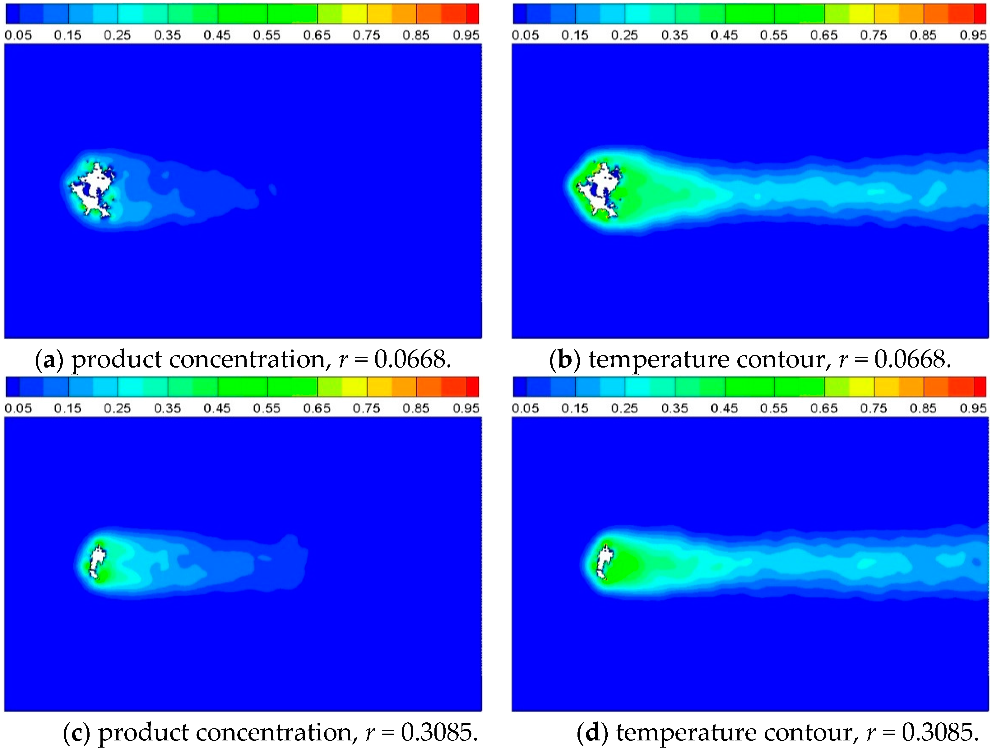
In order to obtain the influence of reaction probability on the process evolution, the value of K^* was set to be 0.5 and 1.5, and the reaction probability was determined as 0.3085 and 0.0668 according to the normal distribution function. The reaction probability decides the reaction velocity, as Equation (9). The product concentration and temperature contour around the cylinder at t = 2500 are shown as Figure 13. 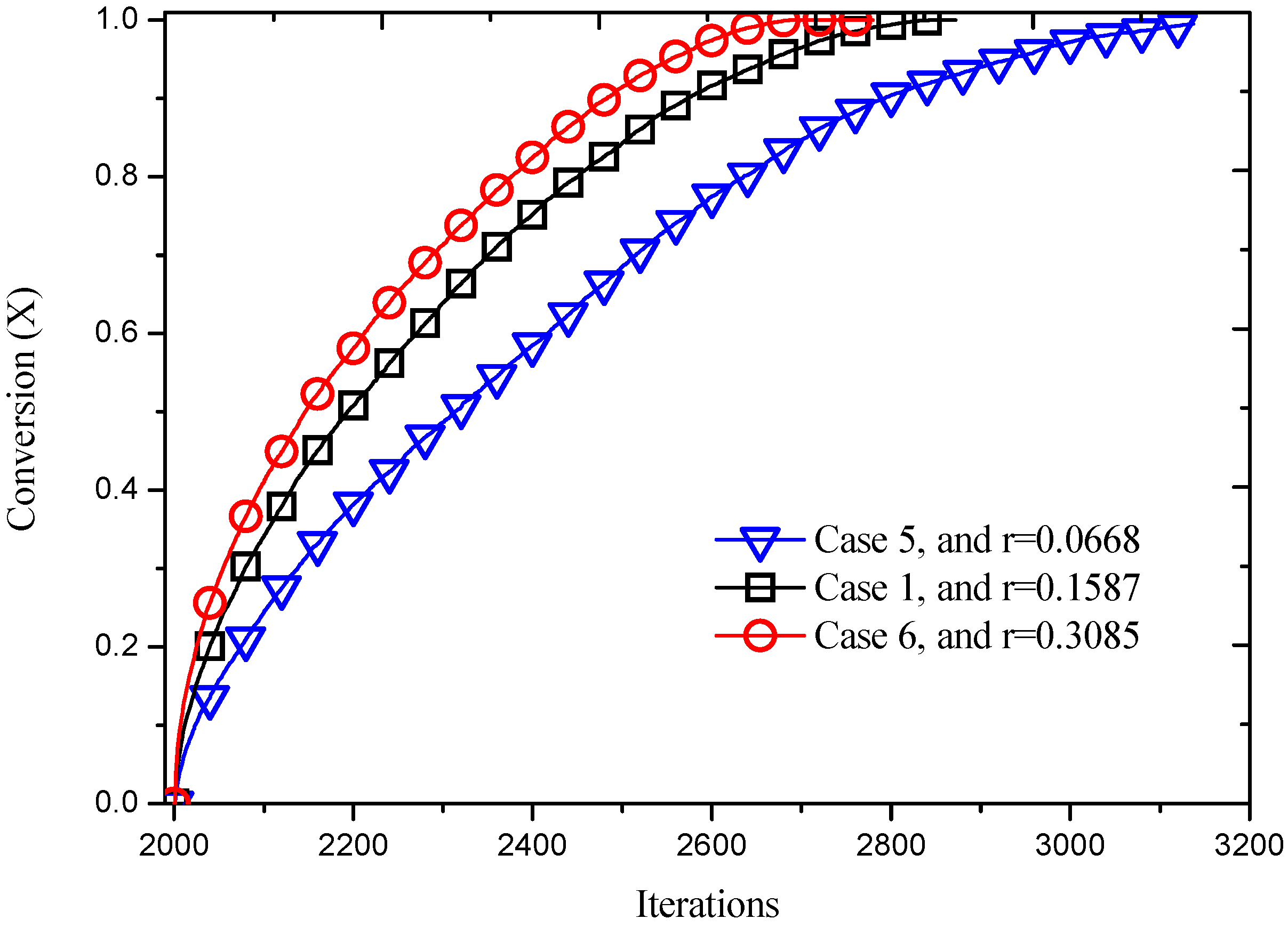It can be obviously noted that the reaction processes faster with a higher value of probability, which also can be seen from Figure 14. The conversion increases as reacting time advances and reaction probability increases. For instance, the complete reaction time increases from 696 iterations to 1140 iterations when the reaction probability decreases from 0.3085 to 0.0668.

Figure 13. Product concentration and temperature contour of Case 5 and Case 6, where reaction probability is 0.0668 and 0.3085, respectively, and t = 2500.

Figure 13. Product concentration and temperature contour of Case 5 and Case 6, where reaction probability is 0.0668 and 0.3085, respectively, and t = 2500.

Figure 14. Reaction processes with different reaction probabilities.

Figure 14. Reaction processes with different reaction probabilities.

3.2.3. Effect of Inlet Gas Velocity

The equilibrium mean occupation numbers are calculated by Fermi–Dirac distribution, as follows

$$n_i^{eq}=\frac{1}{1+\exp (h+q\mathbf{·}{c}_i)}$$

(17)

where h is a real number and $q$ is a D-dimensional vector. The two parameters are termed as Lagrange multipliers. For simplification, the Lagrange multipliers of the equilibrium distributions for lattice gas automata can be obtain by the algebra formula [9]

$$n_i(u)=d+2d{c}_i\mathbf{·}u+2d\frac{1-2d}{1-d}{c}_{i\alpha }^2{u}_{\alpha }^2-d\frac{1-2d}{1-d}{u}^2$$

(18)

where d is equal to $\rho /7$ for FHP-II, and $u$ is the node velocity. Thus, the variable $n_i$ at the inlet nodes can be initialized by Equation (18) with a given particle density d and a node velocity $u$.

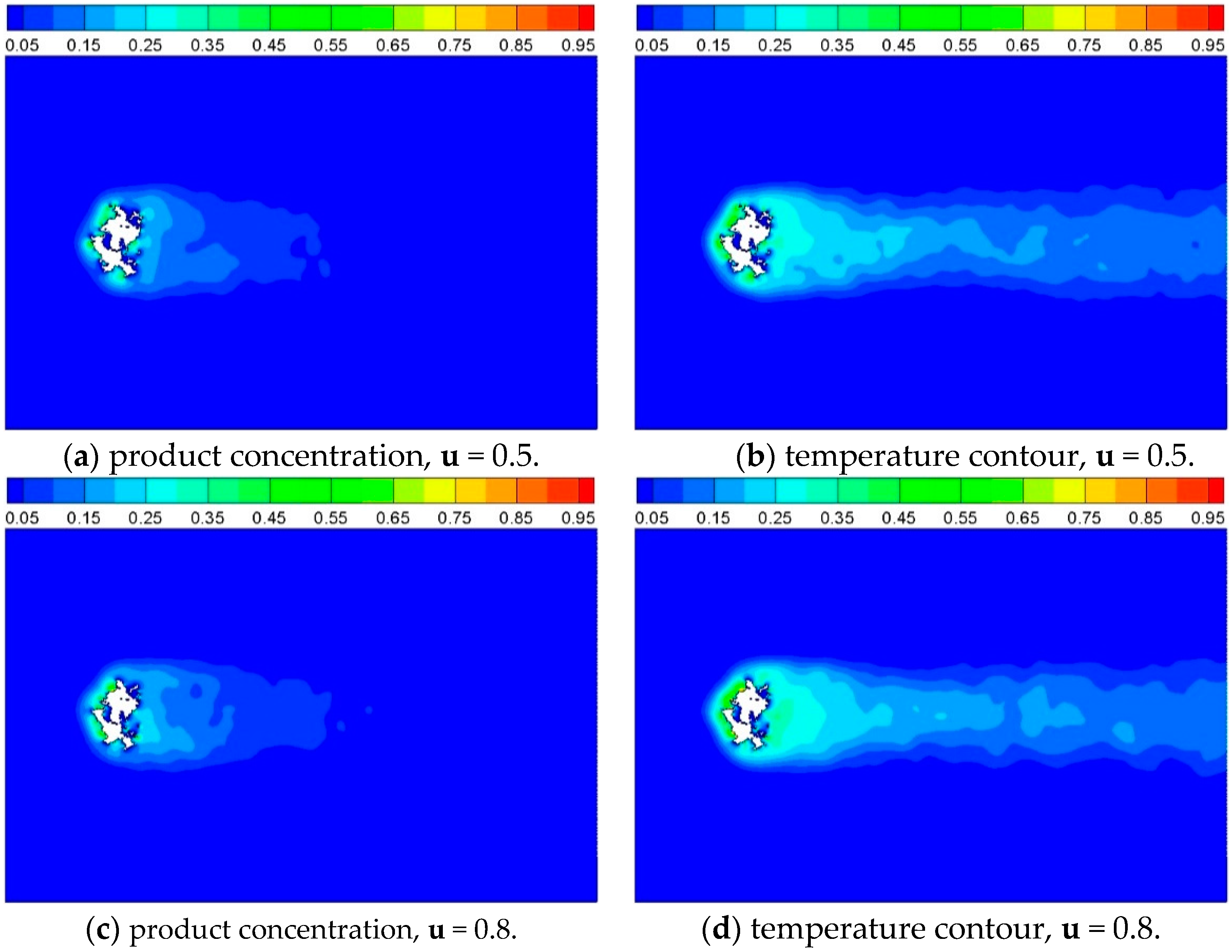
For this section, the effect of velocity at inlet on the reaction process is discussed, and the parameters are listed in Table 1, as Cases 1, 7 and 8. Particle density ρ is fixed as 1.0 for all numerical computation cases, thus d is equal to 1/7. 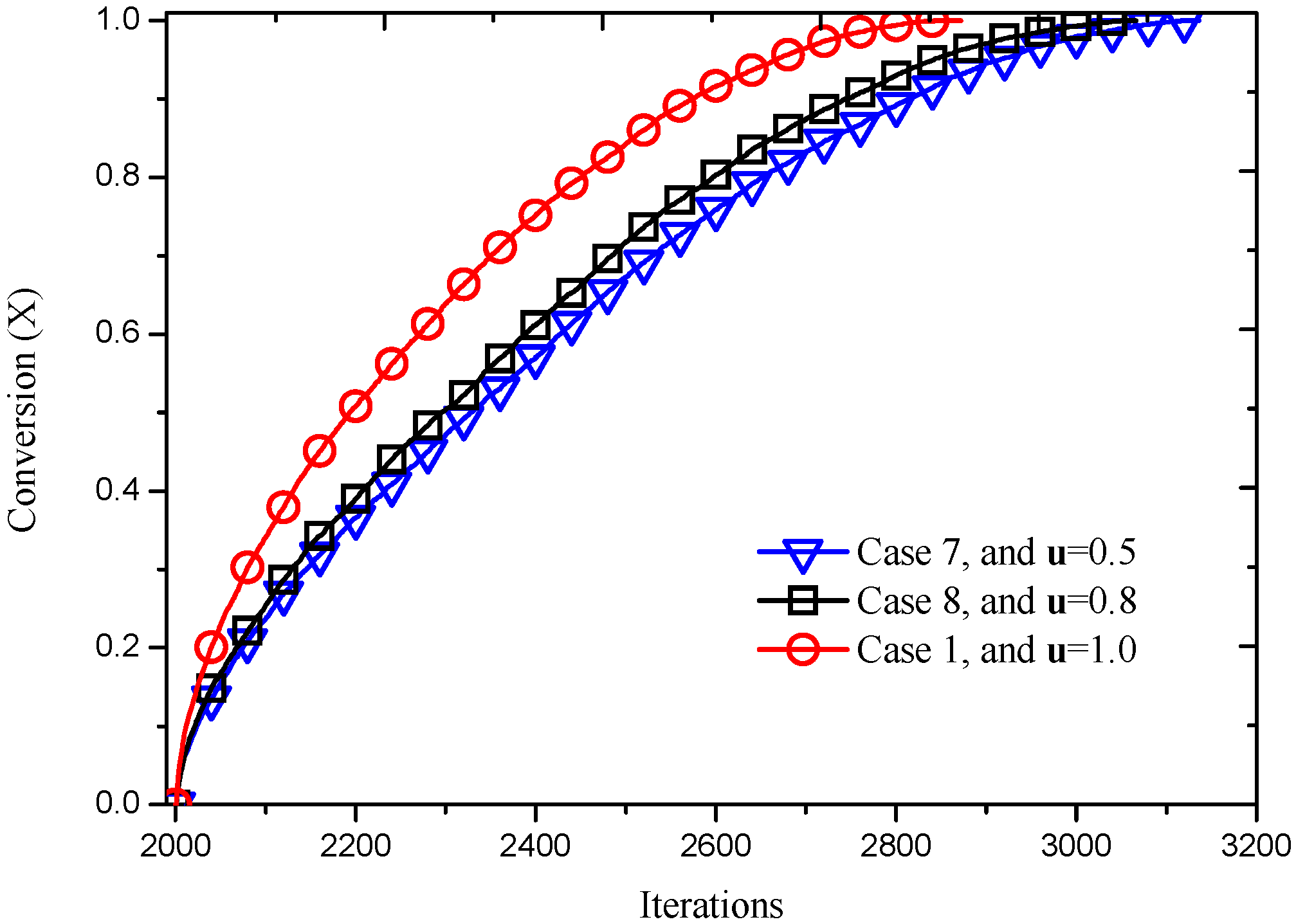The product and temperature contour of cases with different inlet velocities are shown as Figure 15, it can be seen that Case 8 reacts faster than Case 7 and slower than Case 1 compared with Figure 11a, indicating that the reaction velocity increases as the velocity at inlet increases. This information can also be obtained from the dependence of conversion on the reacting time, as shown in Figure 16, which shows that the extent of conversion increases with increasing reacting time, as well as inlet velocity. This agrees well with the theories of surface reaction in gas–solid systems, such as unreacted shrinking core model [36] and pore model [37], which indicate that the increase of gas velocity promotes the collision between gas particles as well as between gas particles and solid sites, facilitating the diffusion and external dispersion of reactant and product.

Figure 15. Product concentration and temperature contour of Case 7 and Case 8, where inlet gas velocity is 0.5 and 0.8, respectively, and t = 2500 iterations.

Figure 15. Product concentration and temperature contour of Case 7 and Case 8, where inlet gas velocity is 0.5 and 0.8, respectively, and t = 2500 iterations.

Figure 16. Reaction processes at different inlet velocities.

Figure 16. Reaction processes at different inlet velocities.

4. Conclusions

A two-dimensional lattice gas automata model is developed to simulate the flow, heat transfer and chemical reaction around and through porous cylinders constructed by QSGS algorithm. In this model, two additional particle properties, i.e., particle type and energy state, are introduced to account for involved chemical species and fluid temperature, respectively. Heat transfer on the interface of gas–solid is then simulated by the change of gas particle energy state at impact. A chemical reaction scheme based on collision theory is developed, where chemical reaction is also interpreted as the change of particle type according to the probability of reaction.

By controlling the construction parameters of the QSGS method, porous cylinders of different pore sizes, solid agglomeration, porosity and surface to mass ratio are generated for the investigation. Their effects, together with that of reaction probability and inlet fluid velocity on the profiles of temperature, solid conversion rate, and reaction product concentration, are discussed. Numerical results indicate that cylinders with a higher porosity, larger pore size, and more surface area to mass ratio react with gas particles faster. Moreover, the reaction velocity increases with increasing reaction probability as well as gas velocity at inlet. These results agree well with the basic theories of the gas dispersion, pore diffusion, and solid surface reaction. The proposed LGA model is therefore believed to provide a prospective modeling strategy for describing gas–solid chemical reaction occurring at complex boundaries from the viewpoint of mesoscopic level.

References

1. Yang, C.; Thovert, J.-F.; Debenest, G. Upscaling of mass and thermal transports in porous media with heterogeneous combustion reactions. Int. J. Heat Mass Transf. 2015, 84, 862–875. [Google Scholar]
2. Mahmud, S.; Fraser, R.A. Free convection and irreversibility analysis inside a circular porous enclosure. Entropy 2003, 5, 358–365. [Google Scholar] [CrossRef]
3. Liu, H.; Patil, P.R.; Narusawa, U. On Darcy-Brinkman equation: Viscous flow between two parallel plates packed with regular square arrays of cylinders. Entropy 2007, 9, 118–131. [Google Scholar] [CrossRef]
4. Makinde, O.D.; Eegunjobi, A.S. Entropy generation in a couple stress fluid flow through a vertical channel filled with saturated porous media. Entropy 2013, 15, 4589–4606. [Google Scholar] [CrossRef]
5. Li, M.; Wu, Y.; Zhao, Z. Effect of endothermic reaction mechanisms on the coupled heat and mass transfers in a porous packed bed with Soret and Dufour effects. Int. J. Heat Mass Transf. 2013, 67, 164–172. [Google Scholar] [CrossRef]
6. Li, X.; Cai, J.; Xin, F.; Huai, X.; Guo, J. Lattice Boltzmann simulation of endothermal catalytic reaction in catalyst porous media. Appl. Therm. Eng. 2013, 50, 1194–1200. [Google Scholar] [CrossRef]
7. Machado, R. Numerical simulations of surface reaction in porous media with lattice Boltzmann. Chem. Eng. Sci. 2012, 69, 628–643. [Google Scholar] [CrossRef]
8. Xin, F.; Li, X.-F.; Xu, M.; Huai, X.-L.; Cai, J.; Guo, Z.-X. Simulation of gas exothermic chemical reaction in porous media reactor with lattice Boltzmann method. J. Therm. Sci. 2013, 22, 42–47. [Google Scholar] [CrossRef]
9. Wolf-Gladrow, D.A. Lattice-Gas Cellular Automata and Lattice Boltzmann Models; Springer: Berlin/Heidelberg, Germany, 2000. [Google Scholar]
10. McNamara, G.R.; Garcia, A.L.; Alder, B.J. Stabilization of thermal lattice Boltzmann models. J. Statist. Phys. 1995, 81, 395–408. [Google Scholar] [CrossRef]
11. McCarthy, J.F. Flow through arrays of cylinders: Lattice gas cellular automata simulations. Phys. Fluids 1994, 6, 435–437. [Google Scholar] [CrossRef]
12. Vogeler, A.; Wolf-Gladrow, D.A. Pair interaction lattice gas simulations: Flow past obstacles in two and three dimensions. J. Statist. Phys. 1993, 71, 163–190. [Google Scholar] [CrossRef]
13. Eissler, W.; Drtina, P.; Frohn, A. Cellular automata simulation of flow around chains of cylinders. Int. J. Numer. Methods Eng. 1992, 34, 773–791. [Google Scholar] [CrossRef]
14. Dab, D.; Lawniczak, A.; Boon, J.-P.; Kapral, R. Cellular-automaton model for reactive systems. Phys. Rev. Lett. 1990, 64, 2462–2465. [Google Scholar] [CrossRef] [PubMed]
15. Boon, J.P.; Dab, D.; Kapral, R.; Lawniczak, A. Lattice gas automata for reactive systems. Phys. Rep. 1996, 273, 55–147. [Google Scholar] [CrossRef]
16. Weimar, J.R. Cellular automata for reaction-diffusion systems. Parallel Comput. 1997, 23, 1699–1715. [Google Scholar] [CrossRef]
17. Seybold, P.G.; Kier, L.B.; Cheng, C.-K. Simulation of first-order chemical kinetics using cellular automata. J. Chem. Inf. Comput. Sci. 1997, 37, 386–391. [Google Scholar] [CrossRef]
18. Seybold, P.G.; Kier, L.B.; Cheng, C.-K. Stochastic cellular automata models of molecular excited-state dynamics. J. Phys. Chem. A 1998, 102, 886–891. [Google Scholar] [CrossRef]
19. Seybold, P.G.; Kier, L.B.; Cheng, C.-K. Aurora borealis: Stochastic cellular automata simulations of the excited-state dynamics of oxygen atoms. Int. J. Quantum Chem. 1999, 75, 751–756. [Google Scholar] [CrossRef]
20. Neuforth, A.; Seybold, P.G.; Kier, L.B.; Cheng, C.-K. Cellular automata models of kinetically and thermodynamically controlled reactions. Int. J. Chem. Kinet. 2000, 32, 529–534. [Google Scholar] [CrossRef]
21. Roberts, J.D.; Caserio, M.C. Basic Principles of Organic Chemistry, 2nd ed.; WA Benjamin: Menlo Park, CA, USA, 1977. [Google Scholar]
22. Lin, K.-C. Understanding product optimization: Kinetic versus thermodynamic control. J. Chem. Educ. 1988, 65, 857–860. [Google Scholar] [CrossRef]
23. Hollingsworth, C.A.; Seybold, P.G.; Kier, L.B.; Cheng, C.-K. First-order stochastic cellular automata simulations of the Lindemann mechanism. Int. J. Chem. Kinet. 2004, 36, 230–237. [Google Scholar] [CrossRef]
24. Lindemann, F.A.; Arrhenius, S.; Langmuir, I.; Dhar, N.R.; Perrin, J.; McC. Lewis, W.C. Discussion on “the radiation theory of chemical action”. Trans. Faraday Soc. 1922, 17, 598–606. [Google Scholar] [CrossRef]
25. Frisch, U.; d’Humières, D.; Hasslacher, B.; Lallemand, P.; Pomeau, Y.; Rivet, J.-P. Lattice gas hydrodynamics in two and three dimensions. Complex Syst. 1987, 1, 649–707. [Google Scholar]
26. Zheng, Z.; Gao, X. Lattice gas automata method for modeling fluid flow and heat transfer in metallurgical porous media. Acta Met. Sin. 2000, 36, 433–437. [Google Scholar]
27. Bresolin, C.S.; Oliveira, A.A.M. An algorithm based on collision theory for the lattice Boltzmann simulation of isothermal mass diffusion with chemical reaction. Comput. Phys. Commun. 2012, 183, 2542–2549. [Google Scholar] [CrossRef]
28. Baercor, T.; Mayer, P.M. Statistical Rice–Ramsperger–Kassel–Marcus quasiequilibrium theory calculations in mass spectrometry. J. Am. Soc. Mass Spectrom. 1997, 8, 103–115. [Google Scholar] [CrossRef]
29. Moon, J.H.; Oh, J.Y.; Kim, M.S. A systematic and efficient method to estimate the vibrational frequencies of linear peptide and protein ions with any amino acid sequence for the calculation of Rice–Ramsperger–Kassel–Marcus rate constant. J. Am. Soc. Mass Spectrom. 2006, 17, 1749–1757. [Google Scholar] [CrossRef] [PubMed]
30. Moon, J.H.; Sun, M.; Kim, M.S. Efficient and reliable calculation of Rice–Ramsperger–Kassel–Marcus unimolecular reaction rate constants for biopolymers: Modification of Beyer–Swinehart algorithm for degenerate vibrations. J. Am. Soc. Mass Spectrom. 2007, 18, 1063–1069. [Google Scholar] [CrossRef] [PubMed]
31. Wichura, M.J. Algorithm as 241: The percentage points of the normal distribution. J. R. Stat. Soc. 1988, 37, 477–484. [Google Scholar] [CrossRef]
32. Lecca, P.; Laurenzi, I.; Jord, F. Deterministic Versus Stochastic Modelling in Biochemistry and Systems Biology; Woodhead Publishing: Cambridge, UK, 2013. [Google Scholar]
33. Chen, H.; Zheng, Z.; Chen, Z.; Bi, X.T. Simulation of flow and heat transfer around a heated stationary circular cylinder by lattice gas automata. Powder Technol. 2015. [Google Scholar] [CrossRef]
34. Wang, M.; Wang, J.; Pan, N.; Chen, S. Mesoscopic predictions of the effective thermal conductivity for microscale random porous media. Phys. Rev. E 2007, 75, 036702. [Google Scholar] [CrossRef] [PubMed]
35. Chen, L.; Wu, G.; Holby, E.F.; Zelenay, P.; Tao, W.-Q.; Kang, Q. Lattice Boltzmann pore-scale investigation of coupled physical-electrochemical processes in C/Pt and non-precious metal cathode catalyst layers in proton exchange membrane fuel cells. Electrochim. Acta 2015, 158, 175–186. [Google Scholar] [CrossRef]
36. Homma, S.; Ogata, S.; Koga, J.; Matsumoto, S. Gas–solid reaction model for a shrinking spherical particle with unreacted shrinking core. Chem. Eng. Sci. 2005, 60, 4971–4980. [Google Scholar] [CrossRef]
37. Petersen, E.E. Reaction of porous solids. AIChE J. 1957, 3, 443–448. [Google Scholar] [CrossRef]