Proportionate Minimum Error Entropy Algorithm for Sparse System Identification

Abstract

Sparse system identification has received a great deal of attention due to its broad applicability. The proportionate normalized least mean square (PNLMS) algorithm, as a popular tool, achieves excellent performance for sparse system identification. In previous studies, most of the cost functions used in proportionate-type sparse adaptive algorithms are based on the mean square error (MSE) criterion, which is optimal only when the measurement noise is Gaussian. However, this condition does not hold in most real-world environments. In this work, we use the minimum error entropy (MEE) criterion, an alternative to the conventional MSE criterion, to develop the proportionate minimum error entropy (PMEE) algorithm for sparse system identification, which may achieve much better performance than the MSE based methods especially in heavy-tailed non-Gaussian situations. Moreover, we analyze the convergence of the proposed algorithm and derive a sufficient condition that ensures the mean square convergence. Simulation results confirm the excellent performance of the new algorithm.

1. Introduction

Sparse system identification is an active research area at present, which finds various real-world applications in network echo cancelation, wireless multipath channels, underwater acoustic communications, and so on [1,2]. A system is qualitatively classified as a sparse system if only a small percentage of coefficients are active, while other coefficients are insignificant (i.e., equal or close to zero). It is worth noting that in compressive sensing and sparse coding, the term “sparse vector” usually means that most of the elements are exactly zero. In system identification and adaptive filtering, however, the term “sparse system (or filter)” in general means that most of the coefficients are equal or close to zero. For a sparse system, classic adaptive filtering algorithms like least mean square (LMS) and normalized LMS (NLMS) [3] may perform poorly in terms of steady state excess mean square error and convergence speed due to not using the a priori knowledge, especially in applications with long sparse systems. As a new scheme, the proportionate normalized least mean square (PNLMS) [4], which updates each filter coefficient in proportion to the magnitude of its estimate, has recently received a great deal of attention, and can perform much better than the conventional NLMS in the identification of sparse systems. Several improvements of the PNLMS algorithm have been proposed [5,6,7,8]. Moreover, several proportionate-type affine projection algorithms (APAs) were also developed [9,10,11,12].

Most of the existing proportionate-type adaptive algorithms (such as PNLMS) are developed based on the well-known mean square error (MSE) criterion. The MSE is computationally simple and mathematically tractable, and optimal when data are Gaussian. However, when the data are non-Gaussian (especially when data are disturbed by impulsive noises or containing large outliers), the MSE may be a poor descriptor of optimality. Man-made low frequency atmospheric noises and lighting spikes in natural phenomena can be described more accurately using non-Gaussian noise models [13,14]. From a statistical point of view, MSE only takes into account the second-order statistics, which is insufficient to capture all possible information from data. As a result, in non-Gaussian situations, the proportionate-type NLMS algorithms may perform poorly especially in the presence of impulsive noises.

Information theoretic learning (ITL) provides an appropriate framework for dealing with non-Gaussian signal processing [15,16]. In ITL, the quadratic Renyi’s entropy of the error was proposed as an alternative to MSE. With nonparametric Parzen window approach, the entropy can be easily estimated from the samples. Under the minimum error entropy (MEE) criterion, an adaptive system can be trained such that the error entropy between the model and unknown system is minimized [17,18,19,20,21,22,23,24,25]. Since entropy can capture higher-order statistics and information content of signals rather than simply their energy, the MEE based adaptive algorithms may achieve significant performance improvements in non-Gaussian situations. In this work, we propose a novel proportionate algorithm for sparse system identification, called the proportionate minimum error entropy (PMEE) algorithm. Instead of using the MSE criterion, the new algorithm is derived based on the MEE criterion. The PMEE algorithm may perform much better than the PNLMS when identifying a sparse system with non-Gaussian noises. In a recent paper [26], we proposed three sparse adaptive filtering algorithms under MEE criterion, namely ZAMEE, RZAMEE, and CIMMEE, which are derived by incorporating a sparsity penalty term into the MEE criterion. These algorithms also perform well for sparse system identification with non-Gaussian noises. However, simulation results in this work show that PMEE can outperform them.

The rest of the paper is organized as follows. In Section 2, after briefly introducing the MEE criterion, we derive the PMEE algorithm. In Section 3, we carry out the mean square convergence analysis. In Section 4, we present simulation results to confirm the excellent performance of the PMEE. Finally, In Section 5, we give the conclusion.

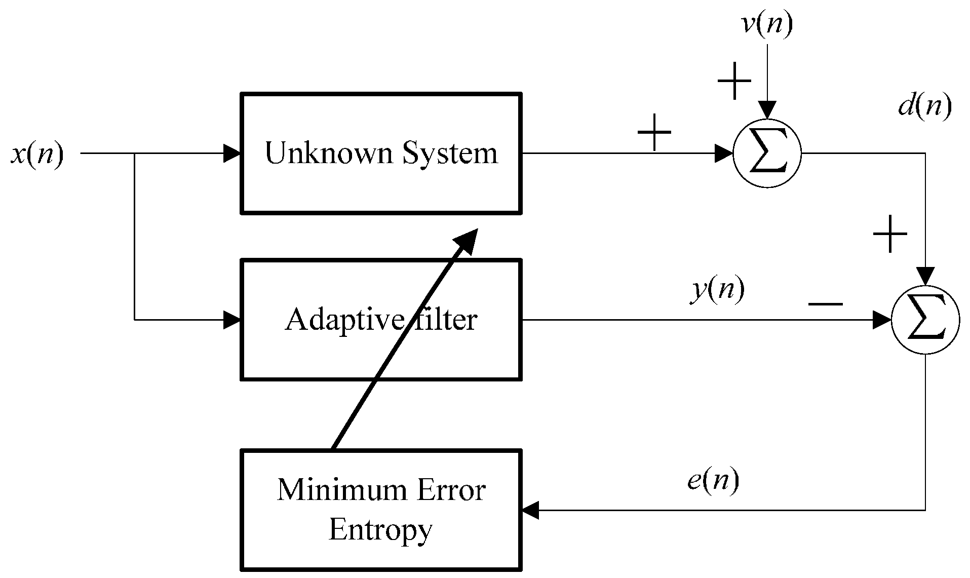
2. Proportionate Minimum Error Entropy Algorithm

2.1. Minimum Error Entropy Criterion

Figure 1 depicts an adaptive filtering scheme under MEE criterion. According to Figure 1, the adaptive filtering can be formulated as minimizing the error entropy between the filter output and the desired response. Since entropy quantifies the average uncertainty or dispersion of a random variable, its minimization makes the error concentrated. Consider a linear system where the desired signal is generated by:

$$d(n)=W^{*T}X(n)+v(n)$$

(1)

where $X(n)={\left[x_{n-M+1},\cdots ,x_{n-1},x_n)\right]}^T$ denotes the input vector at instant $n$, $W^{*}={[w_1^{*},w_2^{*},\cdots ,w_M^{*}]}^T$ denotes the weight (parameter) vector of an finite impulse response (FIR) channel with $M$ being the memory size, ${\rm T}$ denotes the transpose operator, and $v(n)$ stands for the interference or measurement noise. Assume that the adaptive filter is also an FIR filter with weight vector $W(n)={[w_1(n),w_2(n),\cdots ,w_M(n)]}^T$. Then the filtering error is:

$$e(n)=d(n)-y(n)=d(n)-W^T(n)X(n)$$

(2)

where $y(n)$ is the output of the adaptive filter at instant $n$. Let the filtering error be a random variable with probability density function (PDF) $p_e(.)$. The quadratic Renyi’s entropy of error is:

$$H_{R2}(e)=-\log {\displaystyle \int p_e^2(\text{ξ})d\text{ξ}}\text{=}-\log V(e)$$

(3)

where $V(e)={\displaystyle \int p_e^2(\text{ξ})d\text{ξ}}$ is named the quadratic information potential (QIP) [17,18]. In practical applications, however, an analytical expression of the error entropy is not available in general; one has to estimate it directly from the error samples. By the Parzen window approach, the error PDF can be estimated as:

$$p_e(e)=\frac{1}{N}{\displaystyle \sum _{i=1}^N{\kappa }_{\mathbf{\text{σ}}}(e-e(i))}$$

(4)

where $N$ is the samples number, ${\kappa }_{\mathbf{\text{σ}}}$ denotes a kernel function with bandwidth $\text{σ}$, satisfying ${\kappa }_{\text{σ}}(x)\ge 0$, and ${\displaystyle \int {\kappa }_{\text{σ}}(x)dx}=1$. The most popular kernel function used in ITL is the Gaussian kernel:

$${\kappa }_{\text{σ}}(x)=\frac{1}{\mathbf{\text{σ}}\sqrt{2\pi }}\exp (-\frac{x^2}{2{\mathbf{\text{σ}}}^2})$$

(5)

Figure 1. Adaptive filtering under MEE criterion.

Figure 1. Adaptive filtering under MEE criterion.

In the rest of the paper, unless mentioned otherwise, we will use the Gaussian kernel. Combining Equations (3) and (4) yields:

$$\begin{array}{l}{H}_{R2}(e)\approx -\log {\displaystyle \int (\frac{1}{N}{\displaystyle \sum _{i=1}^N{\kappa }_{\text{σ}}(e-e(i))}{)}^{2}de}\\ \text{ =}-\log \frac{1}{N^2}{\displaystyle \sum _{i=1}^N{\displaystyle \sum _{j=1}^N{\displaystyle \int {\kappa }_{\text{σ}}(e-e(i)){\kappa }_{\text{σ}}(e-e(j))d}e}}\\ \text{ =}-\log \frac{1}{N^2}{\displaystyle \sum _{i=1}^N{\displaystyle \sum _{j=1}^N{\kappa }_{\text{σ}\sqrt{2}}(e(i)-e(j))}}\end{array}$$

(6)

One can easily obtain:

$$V(e)\approx \frac{1}{N^2}{\displaystyle \sum _{i=1}^N{\displaystyle \sum _{j=1}^N{\kappa }_{\text{σ}\sqrt{2}}(e(i)-e(j))}}$$

(7)

Obviously, minimizing the quadratic Renyi entropy is equivalent to maximizing the QIP. Thus, the optimal weight vector under MEE can be formulated as:

$$W_{opt}=\underset{W}{\arg \max }V(e)$$

(8)

2.2. Proportionate Minimum Error Entropy

Before presenting the PMEE algorithm, a general form of the PNLMS-type algorithms is revisited. Generally, the weight update equation of the PNLMS-type algorithms can be expressed as [4,8]:

$$W(n+1)=W(n)+\frac{\text{μ}G(n)e(n)X(n)}{X^T(n)G(n)X(n)+\text{δ}}$$

(9)

where $\text{μ}$ is a step size parameter, $\text{δ}>0$ is a regularization parameter that prevents division by zero in Equation (9) and stabilizes the solution, $G(n)$ is a diagonal matrix that modifies the step size of each tap according to a specific rule. In general, the matrix $G(n)$ is given by:

$$G(n)=diag(g_1(n),g_2(n),\cdots ,g_M(n))$$

(10)

where:

$$g_l(n)=\frac{{\varpi }_l(n)}{{\displaystyle \sum _{i=1}^M{\varpi }_i(n)}}1\le l\le M$$

(11)

$${\varpi }_l(n)=\max \left[\text{ε}\max \left\{\varphi ,\left|w_1(n)\right|,\cdots \left|w_M(n)\right|\right\},\left|w_l(n)\right|\right]$$

(12)

The parameter $\text{ε}$ prevents the coefficients from stalling when they are much smaller than the largest one. The parameter $\varphi$ is an initialization parameter that helps to prevent stalling of the weight updating at the initial stage when all the taps are initialized to zero.

To develop the PMEE algorithm for sparse system identification, we use the error entropy instead of the squared error as the adaptation cost. According to Equation (8), a steepest ascent algorithm for estimating the weight vector can be derived as:

$$W(n+1)=W(n)+\text{μ}\nabla V(e(n))$$

(13)

where $\nabla V(e(n))$ denotes the gradient of the QIP with respect to the weight vector, given by:

$$\begin{array}{l}\nabla V(e(n))=\frac{\partial V(e(n))}{\partial W(n)}=\frac{\partial }{\partial W(n)}\left(\frac{1}{L^2}{\displaystyle \sum _{i=n-L+1}^n{\displaystyle \sum _{j=n-L+1}^n{\kappa }_{\text{σ}\sqrt{2}}(\text{Δ}e(i,j))}}\right)\\ \text{ =}\frac{1}{2L^2{\text{σ}}^2}{\displaystyle \sum _{i=n-L+1}^n{\displaystyle \sum _{j=n-L+1}^n\left[{\kappa }_{\text{σ}\sqrt{2}}(\text{Δ}e(i,j))(\text{Δ}e(i,j))\left(\frac{\partial y(i)}{\partial W(n)}-\frac{\partial y(j)}{\partial W(n)}\right)\right]}}\\ \text{ =}\frac{1}{2L^2{\text{σ}}^2}{\displaystyle \sum _{i=n-L+1}^n{\displaystyle \sum _{j=n-L+1}^n\left[{\kappa }_{\text{σ}\sqrt{2}}(\text{Δ}e(i,j))(\text{Δ}e(i,j))\left(X(i)-X(j)\right)\right]}}\end{array}$$

(14)

where $\text{Δ}e(i,j)=e(i)-e(j)$, and $L$ denotes the sliding data length. Hence, inspired by the PNLMS-type algorithms, we propose the following weight update equation:

$$\begin{array}{ll}W(n+1)& =W(n)+\text{μ}G(n)\nabla V(e(n))\\ & =W(n)+G(n)\frac{\text{μ}}{2L^2{\text{σ}}^2}{\displaystyle \sum _{i=n-L+1}^n{\displaystyle \sum _{j=n-L+1}^n\left[{\kappa }_{\text{σ}\sqrt{2}}(\text{Δ}e(i,j))(\text{Δ}e(i,j))\left(X(i)-X(j)\right)\right]}}\end{array}$$

(15)

where $G(n)$ is determined by Equations (10)–(12). This algorithm is referred to as the PMEE algorithm.

Remark 1. 

Obviously, one can also propose a normalized version of PMEE by dividing the term $X^T(n)G(n)X(n)+\text{δ}$, just like Equation (9). However, our simulation results indicate that the normalized PMEE performs well only when the underlying system is extremely sparse. Thus, in this work, we don’t consider the normalized PMEE. Maybe other updating laws may exist that can provide possibly better result, but this is beyond the scope of this work.

3. Mean Square Convergence Analysis

3.1. Energy Conservation Relation

We rewrite Equation (2) in a form of block data:

$$\overrightarrow{e}(n)=\overrightarrow{d}(n)-\overrightarrow{y}(n)=\overrightarrow{d}(n)-\text{χ}(n)W(n)$$

(16)

where $\overrightarrow{e}(n)={[e(n-L+1),\cdots ,e(n)]}^T$, $\overrightarrow{d}(n)={[d(n-L+1),\cdots ,d(n)]}^T$, $\overrightarrow{y}(n)={[y(n-L+1),\cdots ,y(n)]}^T$, and $\text{χ}(n)={[X(n-L+1),X(n-L+2),\cdots ,X(n)]}^T$ stands for an $L\times M$ input matrix. Define the a priori error vector ${\overrightarrow{e}}_a(\text{n})$ and a posteriori error vector ${\overrightarrow{e}}_p(\text{n})$ as follows:

$$\{\begin{array}{c}{\overrightarrow{e}}_a(n)={[e_a(n-L+1),\cdots ,e_a(n)]}^T=\text{χ}(n)\tilde{W}(n)\\ {\overrightarrow{e}}_p(n)={[e_p(n-L+1),\cdots ,e_p(n)]}^T=\text{χ}(n)\tilde{W}(n+1)\end{array}$$

(17)

where $\tilde{W}(n)=W^{*}-W(n)$ is the weight error vector. Then, ${\overrightarrow{e}}_a(\text{n})$ and ${\overrightarrow{e}}_p(\text{n})$ satisfies:

$${\overrightarrow{e}}_p(n)={\overrightarrow{e}}_a(n)+\text{χ}(n)(\tilde{W}(n+1)-\tilde{W}(n))={\overrightarrow{e}}_a(n)-\text{χ}(n)(W(n+1)-W(n))$$

(18)

Now Equation (15) can be rewritten as:

$$W(n+1)=W(n)+\text{μ}G(n){\text{χ}}^T(n)\overrightarrow{h}(\overrightarrow{e}(n))$$

(19)

where $\overrightarrow{h}(\overrightarrow{e}(n))={[h_1(\overrightarrow{e}(n)),h_2(\overrightarrow{e}(n)),\cdots ,h_L(\overrightarrow{e}(n))]}^T$, in which:

$$h_i(\overrightarrow{e}(n))=\frac{\partial J_{MEE}(\overrightarrow{e}(n))}{\partial e(n-L+i)}$$

(20)

To simplify the analysis, below we assume $L=M$. Combining Equations (18) and (19), one can derive:

$$\begin{array}{l}{\overrightarrow{e}}_p(n)={\overrightarrow{e}}_a(n)-\text{μχ}(n)G(n){\text{χ}}^T(n)\overrightarrow{h}(\overrightarrow{e}(n))\\ \Rightarrow {\overrightarrow{e}}_p(n)-{\overrightarrow{e}}_a(n)=-\text{μχ}(n)G^{\ast }(n){(\text{χ}(n)G^{\ast }(n))}^T\overrightarrow{h}(\overrightarrow{e}(n))\\ \Rightarrow {\overrightarrow{e}}_p(n)-{\overrightarrow{e}}_a(n)=-\text{μ}{\rm H}(n){{\rm H}}^T(n)\overrightarrow{h}(\overrightarrow{e}(n))\\ \Rightarrow {\text{R}}^{-1}(n)({\overrightarrow{e}}_p(n)-{\overrightarrow{e}}_a(n))=-\text{μ}\overrightarrow{h}(\overrightarrow{e}(n))\\ \Rightarrow G(n){\text{χ}}^T(n){\text{R}}^{-1}(n)({\overrightarrow{e}}_p(n)-{\overrightarrow{e}}_a(n))=-(W(n+1)-W(n))\\ \Rightarrow G(n){\text{χ}}^T(n){\text{R}}^{-1}(n)({\overrightarrow{e}}_p(n)-{\overrightarrow{e}}_a(n))=\tilde{W}(n+1)-\tilde{W}(n)\end{array}$$

(21)

where $G^{\ast }(n)=diag(\sqrt{g_1(n)},\sqrt{g_2(n)},\cdots ,\sqrt{g_M(n)})$, ${\rm H}(n)=\text{χ}(n)G^{\ast }(n)$, and $\text{R}(n)={\rm H}(n){{\rm H}}^T(n)$ is an $L\times L$-dimensional symmetric matrix. Assume that $\text{R}(n)$ is invertible. Then we obtain:

$$\tilde{W}(n+1)=\tilde{W}(n)+G(n){\text{χ}}^T(n){\text{R}}^{-1}(n)({\overrightarrow{e}}_p(n)-{\overrightarrow{e}}_a(n))$$

(22)

Squaring both sides of Equation (22), we have:

$$\begin{array}{l}{\tilde{W}}^T(n+1)\tilde{W}(n+1)={[\tilde{W}(n)+G(n){\text{χ}}^T(n){\text{R}}^{-1}(n)({\overrightarrow{e}}_p(n)-{\overrightarrow{e}}_a(n))]}^T\\ \times [\tilde{W}(n)+G(n){\text{χ}}^T(n){\text{R}}^{-1}(n)({\overrightarrow{e}}_p(n)-{\overrightarrow{e}}_a(n))]\end{array}$$

(23)

After some simple manipulations, we derive:

$${\Vert \tilde{W}(n+1)\Vert }^2+{\Vert {\overrightarrow{e}}_a(n)\Vert }_{{\Re }^{-1}(n)}^2={\Vert \tilde{W}(n)\Vert }^2+{\Vert {\overrightarrow{e}}_p(n)\Vert }_{{\Re }^{-1}(n)}^2$$

(24)

where $\Re (n)=\chi (n){\chi }^T(n)$, ${\Vert \tilde{W}(n)\Vert }^2={\tilde{W}}^T(n)\tilde{W}(n)$, ${\Vert {\overrightarrow{e}}_a(n)\Vert }_{{\Re }^{-1}(n)}^2={\overrightarrow{e}}_a^T(n){\Re }^{-1}(n){\overrightarrow{e}}_a(n)$, and ${\Vert {\overrightarrow{e}}_p(n)\Vert }_{{\Re }^{-1}(n)}^2={\overrightarrow{e}}_p^T(n){\Re }^{-1}(n){\overrightarrow{e}}_p(n)$. Taking the expectations of the both sides of Equation (24) leads to the energy conservation relation [19,23,26]:

$$E\left[{\Vert \tilde{W}(n+1)\Vert }^2\right]+E\left[{\Vert {\overrightarrow{e}}_a(n)\Vert }_{{\Re }^{-1}(n)}^2\right]=E\left[{\Vert \tilde{W}(n)\Vert }^2\right]+E\left[{\Vert {\overrightarrow{e}}_p(n)\Vert }_{{\Re }^{-1}(n)}^2\right]$$

(25)

where $E\left[{\Vert \tilde{W}(n)\Vert }^2\right]$ is called the weight error power (WEP) at iteration $n$.

3.2. Sufficient Condition for Mean Square Convergence

Based on the energy conservation relation Equation (25), a sufficient condition that guarantees the mean square convergence (i.e., the monotonic decrease of the WEP) can be easily derived. Substituting ${\overrightarrow{e}}_p(n)={\overrightarrow{e}}_a(n)-\text{μχ}(n)G(n){\text{χ}}^T(n)\overrightarrow{h}(\overrightarrow{e}(n))$ into Equation (25), we have:

$$\begin{array}{l}E\left[{\Vert \tilde{W}(n+1)\Vert }^2\right]=E\left[{\Vert \tilde{W}(n)\Vert }^2\right]-2\text{μ}E\left[{\overrightarrow{e}}_a^T(n){\Re }^{-1}(n)\text{χ}(n)G(n){\text{χ}}^T(n)\overrightarrow{h}(\overrightarrow{e}(n))\right]\\ +{\text{μ}}^{2}E\left[{\overrightarrow{h}}^T(\overrightarrow{e}(n)){\text{χ}}^T(n)G(n)\text{χ}(n){\Re }^{-1}(n)\text{χ}(n)G(n){\text{χ}}^T(n)\overrightarrow{h}(\overrightarrow{e}(n))\right]\end{array}$$

(26)

It follows that:

$$\begin{array}{l}E\left[{\Vert \tilde{W}(n+1)\Vert }^2\right]\le E\left[{\Vert \tilde{W}(n)\Vert }^2\right]\\ \iff {\text{ μ}}^{2}E\left[{\overrightarrow{h}}^T(\overrightarrow{e}(n)){\text{χ}}^T(n)G(n)\text{χ}(n){\Re }^{-1}(n)\text{χ}(n)G(n){\text{χ}}^T(n)\overrightarrow{h}(\overrightarrow{e}(n))\right]\\ \le 2\text{μ}E\left[{\overrightarrow{e}}_a^T(n){\Re }^{-1}(n)\text{χ}(n)G(n){\text{χ}}^T(n)\overrightarrow{h}(\overrightarrow{e}(n))\right]\\ \iff \text{ μ}\le \frac{2E\left[\text{ϒ}\right]}{E\left[\text{Θ}\right]}\end{array}$$

(27)

where

$$\text{ϒ}={\overrightarrow{e}}_a^T(n){\Re }^{-1}(n)\text{χ}(n)G(n){\text{χ}}^T(n)\overrightarrow{h}(\overrightarrow{e}(n)),$$

$$\text{Θ}={\overrightarrow{h}}^T(\overrightarrow{e}(n)){\text{χ}}^T(n)G(n)\text{χ}(n){\Re }^{-1}(n)\text{χ}(n)G(n){\text{χ}}^T(n)\overrightarrow{h}(\overrightarrow{e}(n)).$$

Since $\text{μ}\ge 0$, a sufficient condition for the mean square convergence will be:

$$\{\begin{array}{c}E\left[\text{ϒ}\right]>0\\ 0<\text{μ}\le \frac{2E\left[\text{ϒ}\right]}{E\left[\text{Θ}\right]}\end{array}$$

(28)

The above sufficient condition ensures that the WEP will be monotonically decreasing (hence the algorithm will not diverge).

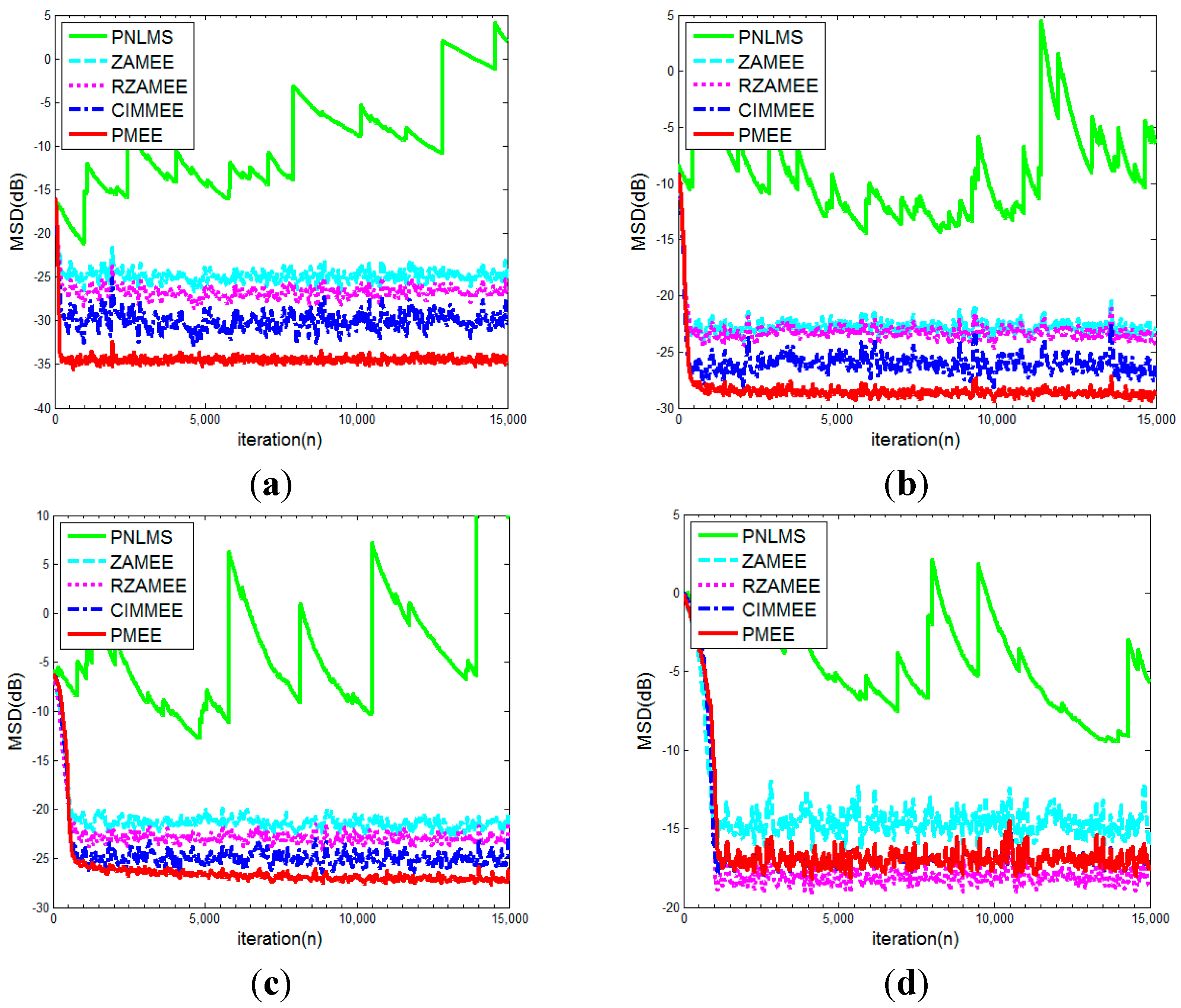
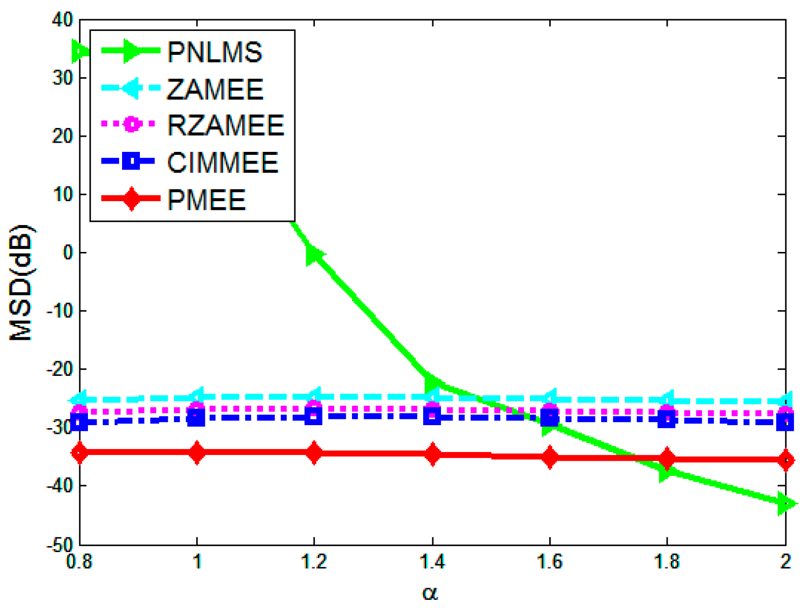
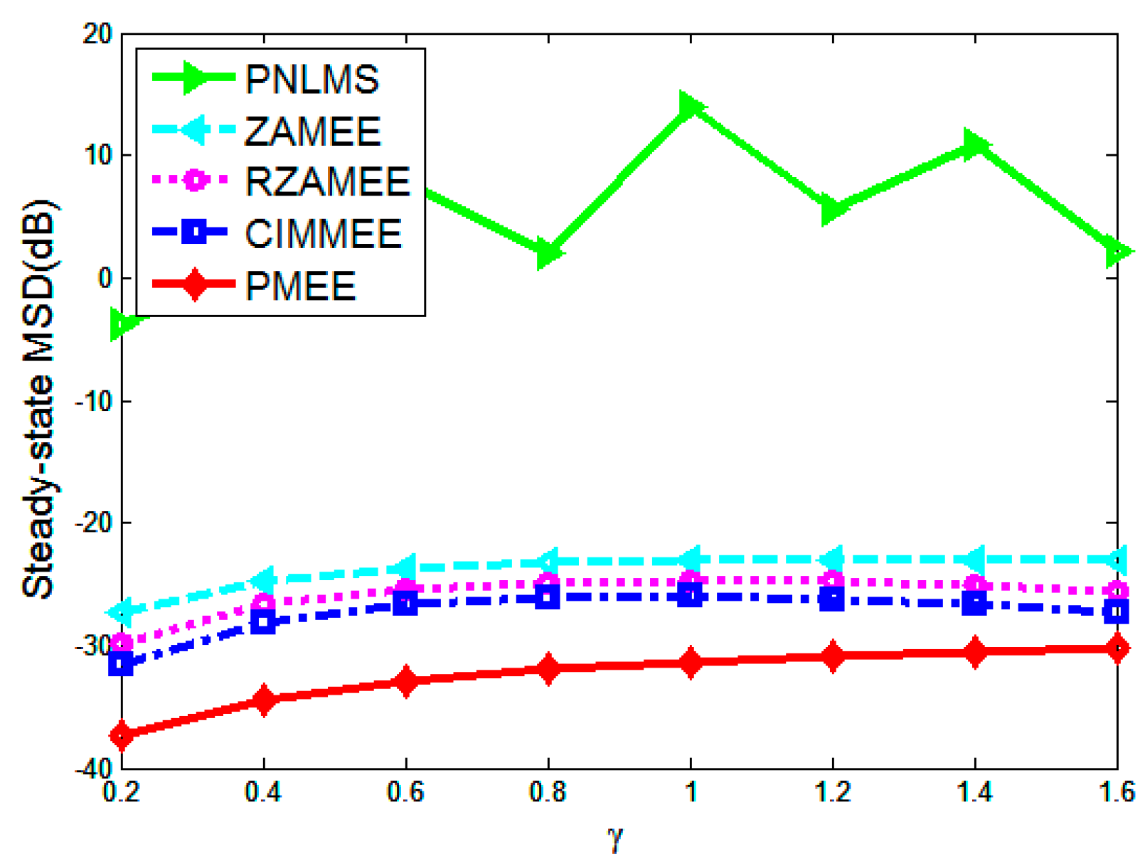
4. Simulation Results

Now we present simulation results about sparse system identification to demonstrate the performance of the PMEE, compared with ZAMEE, RZAMEE, CIMMEE [26] and PNLMS. The mean square deviation (MSD) is used as the performance index, calculated by:

$$\text{MSD=}E\left[{\Vert W^{*}-W(n)\Vert }^2\right]$$

(29)

In order to show the performance of the algorithms in impulsive noise environments, we adopt the alpha-stable distribution [27,28] to generate the disturbance noise, whose characteristic function is:

$$f(t)=\exp \{\text{jδ}t-\text{γ}|t{|}^{\alpha }[1+\text{jβ}\mathrm{sgn}(t)\text{S}(t,\text{α})]\}$$

(30)

in which:

$$\text{S}(t,\text{α})=\{\begin{array}{cc}\tan \frac{\text{απ}}{2},& \text{if α}\ne 1\\ \frac{2}{\text{π}}\log \left|t\right|,& \text{if α}=1\end{array}$$

(31)

where $\text{α}\in (0,2]$ is the characteristic factor, $-\infty <\text{δ}<+\infty$ is the location parameter, $\text{β}\in [-1,1]$; is the symmetry parameter, and $\text{γ}>0$ is the dispersion parameter. This distribution is called a symmetric alpha-stable ($S\text{α}S$) distribution when $\text{β}=0$. We define the parameter vector $V=(\text{α},\text{β},\text{γ},\text{δ})$. In addition, we consider four unknown channels with different parameter vectors:

(a) 

Channel 1:

$$W^{*}=[0,0,0,0,0,0,0,0,1,0,0,0,0,0,0,0,0,0,0,0,0,0,0,0,0,0,0,0,0,0,0,0,0,0,0,0,0,0,0,0]$$

(b) 

Channel 2:

$$W^{*}=[0,0,0,0,0,0,0,1,0,0,0,0,0,0,0,1,0,0,0,0,0,0,0,1,0,0,0,0,0,0,0,1,0,0,0,0,0,0,0,1]$$

(c) 

Channel 3:

$$W^{*}=[0,0,0,1,0,0,0,1,0,0,0,1,0,0,0,1,0,0,0,1,0,0,0,1,0,0,0,1,0,0,0,1,0,0,0,1,0,0,0,1]$$

(d) 

Channel 4:

$$W^{*}=[1,-1,1,-1,1,-1,1,-1,1,-1,1,-1,1,-1,1,-1,1,-1,1,-1,1,-1,1,-1,1,-1,1,-1,1,-1,1,-1,1,-1,1,-1,1,-1,1,-1]$$

Clearly, the four channels (with memory size 40) have different sparsity ratio (1/40, 1/8, 1/4, 1). In all the simulations below, the input signal is a white Gaussian process with zero mean and unit variance. The parameters $\text{ε}$ and $\varphi$ are set at 1/40 and 0.001, respectively. The sliding data length is $L=20$. Simulation results are averaged over 200 independent Monte Carlo runs, and each run has 15,000 iterations.

In the first simulation, the parameter vector $V$ is set at $(1.2,0,0.4,0)$, the kernel width $\text{σ}$ is 1.0, and the step sizes are chosen such that all the algorithms have almost the same initial convergence rate. Figure 2 illustrates the convergence curves for different channels. One can observe: (i) when the system is very sparse (e.g., channel 1 and 2), the PMEE achieves much lower steady-state MSDs than other algorithms; (ii) when the channel is less sparse (e.g., channel 3), the steady-state MSDs of PMEE is still the lowest although there is a little loss in performance; (iii) when the system is completely non-sparse (e.g., channel 4), the performance of PMEE is comparable with CIMMEE. Note that in all the cases, the PNLMS algorithm cannot work since it is very sensitive to impulsive noises.

In the second simulation, we show the performance of the algorithms with different noise parameters (assume that the unknown system is the channel 1). The steady-state MSDs with different $\text{α}$ (0.8,1.0,1.2,1.4,1.6,1.8,2.0) and different $\text{γ}$ (0.2,0.4,0.6,0.8,1.0,1.2,1.4,1.6) are shown in Figure 3 and Figure 4, respectively. Evidently, the PMEE performs very well and achieves the lowest MSDs compared with ZAMEE, RZAMEE, and CIMMEE. The PNLMS performs well (even better than PMEE) only when $\text{α}$ is very close to 2.0. The main reason for this is that, when $\text{α}$ comes near to 2.0, the noise will be approximately Gaussian. Simulation results confirm that the PMEE can effectively identify a sparse system in a non-Gaussian impulsive noise environment.

Figure 2. Convergence curves for different channels: (a) channel 1; (b) channel 2; (c) channel 3; (d) channel 4.

Figure 2. Convergence curves for different channels: (a) channel 1; (b) channel 2; (c) channel 3; (d) channel 4.

In the third simulation, we investigate how the kernel width affects the convergence performance. The noise parameters are set at $V=(1.2,0,0.4,0)$. Simulation results are shown in Figure 5, from which one can see that the kernel width has significant influence on the convergence performance. When the kernel width is too large or too small, the performance will become poor. In a practical application, the kernel width can be manually selected or optimized by trial and error.

Figure 3. Steady-state MSDs with different $\text{α}$ ($\text{γ}=0.4$).

Figure 3. Steady-state MSDs with different $\text{α}$ ($\text{γ}=0.4$).

Figure 4. Steady-state MSDs with different $\text{γ}$ ($\text{α}=1.2$).

Figure 4. Steady-state MSDs with different $\text{γ}$ ($\text{α}=1.2$).

Figure 5. Convergence curves with different kernel widths.

Figure 5. Convergence curves with different kernel widths.

5. Conclusions

In this work, the proportionate minimum error entropy (PMEE) algorithm has been developed to identify a sparse system. Different from the existing proportionate-type adaptive filtering algorithms, such as the proportionate normalized least mean square (PNLMS), PMEE is derived by using the minimum error entropy (MEE) instead of the traditional mean square error (MSE) as the adaptation criterion. Convergence analysis based on energy conservation relation has been carried out, and a sufficient condition for ensuring the mean square stability is obtained. Simulation results have demonstrated the superior performance of the proposed algorithm especially in impulsive non-Gaussian situations.

References

1. Huang, Y.; Benesty, J.; Chen, J. Acoustic MIMO Signal Processing; Springer: New York, NY, USA, 2006. [Google Scholar]
2. Paleologu, C.; Benesty, J.; Ciochina, S. Sparse Adaptive Filters for Echo Cancellation; Morgan and Claypool: San Rafael, CA, USA, 2010. [Google Scholar]
3. Sayed, A.H. Fundamentals of Adaptive Filtering; Wiley: Hoboken, NJ, USA, 2003. [Google Scholar]
4. Duttweiler, D. Proportionate normalized least-mean-squares adaptation in echo cancellers. IEEE Trans. Speech Audio Process. 2000, 8, 508–518. [Google Scholar] [CrossRef]
5. Deng, H.; Doroslovacki, M. Improving convergence of the PNLMS algorithm for sparse impulse response identification. IEEE Signal Process. Lett. 2005, 12, 181–184. [Google Scholar] [CrossRef]
6. Laska, B.N.M.; Goubran, R.A.; Bolic, M. Improved proportionate subband NLMS for acoustic echo cancellation in changing environments. IEEE Signal Process. Lett. 2008, 15, 337–340. [Google Scholar] [CrossRef]
7. Das Chagas de Souza, F.; Seara, R.; Morgan, D.R. An enhanced IAF-PNLMS adaptive algorithm for sparse impulse response identification. IEEE Trans. Signal Process. 2012, 60, 3301–3307. [Google Scholar] [CrossRef]
8. Deng, H.; Doroslovacki, M. Proportionate adaptive algorithms for network echo cancellation. IEEE Trans. Signal Process. 2006, 54, 1794–1803. [Google Scholar] [CrossRef]
9. Paleologu, C.; Ciochină, S.; Benesty, J. An efficient proportionate affine projection algorithm for echo cancellation. IEEE Signal Process. Lett. 2010, 17, 165–168. [Google Scholar] [CrossRef]
10. Yang, J.; Sobelman, G.E. Efficient μ-law improved proportionate affine projection algorithm for echo cancellation. Electron. Lett. 2010, 47, 73–74. [Google Scholar] [CrossRef]
11. Yang, Z.; Zheng, Y.R.; Grant, S.L. Proportionate affine projection sign algorithms for network echo cancellation. IEEE Trans. Audio Speech Lang. Process. 2011, 19, 2273–2284. [Google Scholar] [CrossRef]
12. Zhao, H.; Yu, Y.; Gao, S.; Zeng, X.; He, Z. Memory proportionate APA with individual activation factors for acoustic echo cancellation. IEEE Trans. Audio Speech Lang. Process. 2014, 22, 1047–1055. [Google Scholar] [CrossRef]
13. Plataniotis, K.N.; Androutsos, D.; Venetsanopoulos, A.N. Nonlinear filtering of non-Gaussian noise. J. Intell. Robot. Syst. 1997, 19, 207–231. [Google Scholar] [CrossRef]
14. Weng, B.; Barner, K.E. Nonlinear system identification in impulsive environments. IEEE Trans. Signal Process. 2005, 53, 2588–2594. [Google Scholar] [CrossRef]
15. Principe, J.C. Information Theoretic Learning: Renyi’s Entropy and Kernel Perspectives; Springer: New York, NY, USA, 2010. [Google Scholar]
16. Chen, B.; Zhu, Y.; Hu, J.C.; Jose Principe, J.C. System Parameter Identification: Information Criteria and Algorithms; Elsevier: Amsterdam, The Netherlands, 2013. [Google Scholar]
17. Erdogmus, D.; Principe, J.C. An error-entropy minimization for supervised training of nonlinear adaptive systems. IEEE Trans. Signal Process. 2002, 50, 1780–1786. [Google Scholar] [CrossRef]
18. Erdogmus, D.; Principe, J.C. Convergence properties and data efficiency of the minimum error entropy criterion in adaline training. IEEE Trans. Signal Process. 2003, 51, 1966–1978. [Google Scholar] [CrossRef]
19. Chen, B.; Zhu, Y.; Hu, J. Mean-square convergence analysis of ADALINE training with minimum error entropy criterion. IEEE Trans. Neural Netw. 2010, 21, 1168–1179. [Google Scholar] [CrossRef] [PubMed]
20. Chen, B.; Hu, J.; Pu, L.; Sun, Z. Stochastic gradient algorithm under (h, phi)-entropy criterion. Circuit Syst. Signal Process. 2007, 26, 941–960. [Google Scholar] [CrossRef]
21. Li, C.; Shen, P.; Liu, Y.; Zhang, Z. Diffusion information theoretic learning for distributed estimation over network. IEEE Trans. Signal Process. 2013, 61, 4011–4024. [Google Scholar] [CrossRef]
22. Wolsztynski, E.; Thierry, E.; Pronzato, L. Minimum-entropy estimation in semi-parametric models. Signal Process. 2005, 85, 937–949. [Google Scholar] [CrossRef]
23. Al-Naffouri, T.Y.; Sayed, A.H. Adaptive filters with error nonlinearities: Mean-square analysis and optimum design. EURASIP J. Appl. Signal Process. 2001, 4, 192–205. [Google Scholar] [CrossRef]
24. Chen, B.; Principe, J.C. Some further results on the minimum error entropy estimation. Entropy 2012, 14, 966–977. [Google Scholar] [CrossRef]
25. Chen, B.; Principe, J.C. On the Smoothed Minimum Error Entropy Criterion. Entropy 2012, 14, 2311–2323. [Google Scholar] [CrossRef]
26. Wu, Z.; Peng, S.; Ma, W.; Chen, B.; Principe, J.C. Minimum Error Entropy Algorithm with Sparsity Penalty Constraints. Entropy 2015, 17, 3419–3437. [Google Scholar] [CrossRef]
27. Weng, B.; Barner, K.E. Nonlinear system identification in impulsive environments. IEEE Trans. Signal Process. 2005, 53, 2588–2594. [Google Scholar] [CrossRef]
28. Wang, J.; Kuruoglu, E.E.; Zhou, T. Alpha-stable channel capacity. IEEE Commun. Lett. 2011, 15, 1107–1109. [Google Scholar] [CrossRef]