Information-Theoretic Characterization and Undersampling Ratio Determination for Compressive Radar Imaging in a Simulated Environment

Abstract

Assuming sparsity or compressibility of the underlying signals, compressed sensing or compressive sampling (CS) exploits the informational efficiency of under-sampled measurements for increased efficiency yet acceptable accuracy in information gathering, transmission and processing, though it often incurs extra computational cost in signal reconstruction. Shannon information quantities and theorems, such as source rate-distortion, trans-information and rate distortion theorem concerning lossy data compression, provide a coherent framework, which is complementary to classic CS theory, for analyzing informational quantities and for determining the necessary number of measurements in CS. While there exists some information-theoretic research in the past on CS in general and compressive radar imaging in particular, systematic research is needed to handle issues related to scene description in cluttered environments and trans-information quantification in complex sparsity-clutter-sampling-noise settings. The novelty of this paper lies in furnishing a general strategy for information-theoretic analysis of scene compressibility, trans-information of radar echo data about the scene and the targets of interest, respectively, and limits to undersampling ratios necessary for scene reconstruction subject to distortion given sparsity-clutter-noise constraints. A computational experiment was performed to demonstrate informational analysis regarding the scene-sampling-reconstruction process and to generate phase transition diagrams showing relations between undersampling ratios and sparsity-clutter-noise-distortion constraints. The strategy proposed in this paper is valuable for information-theoretic analysis and undersampling theorem developments in compressive radar imaging and other computational imaging applications.

1. Introduction

Unlike the traditional practice of sampling followed by compression, CS provides a framework for directly acquiring data in compressed form, thus promoting sub-Nyqusit sampling that is more efficient than what is required by the Shannon-Nyquist sampling theorem [1,2,3]. It has been applied to various fields including optical and radar remote sensing [4,5,6,7,8,9,10,11,12,13]. In addition to the assumption made of the sparsity of the scene being sensed and imaged, the working of a CS-radar system relies also on the informational transferability of the measurement matrices in capturing the amount of mutual information in the measurements about the underlying scene and the targets of interest, in particular, and algorithms that can reconstruct the sparse signal from undersampled but information-laden data [8,14,15].

Classic information theory as introduced by Shannon provides the mathematics for the design of transmitter and receiver in a communication system to efficiently and reliably transmit the information from the source to the destination given the characteristics of the source and the channel, and can be applied to address issues, such as data compression, in a wide variety of fields [16,17,18,19]. As this paper focuses on information-theoretic analyses in CS-radar, a brief description of some of the basic concepts in information theory is provided here. The entropy of a source is a lower bound on the average length of the shortest description about it, implying that a description about it can be constructed with average length within 1 bit of the entropy [17]. Relaxing the constraints of recovering the source perfectly, rate distortion function quantifies the amount of information rate required to describe it up to a specific distortion measure, providing the trade-offs between information rates and distortion tolerance. In other words, a rate distortion function quantifies the minimum rate description required to achieve a particular distortion [17]. While entropy and rate distortion are both used to quantify the compressibility of a source, the concept of mutual information is useful for quantification of the amount of information transmitted through measurements concerning the underlying source. By definition, mutual information is the difference between the entropy of a random variable (RV) and its conditional entropy given the knowledge of another conditioning RV. It reflects the reduction in the uncertainty of a RV say a radar scene due to knowledge provided by another RV say a set of radar echo data acquired of the scene. In this paper, mutual information is used interchangeably with trans-information, although there are some conventional differences regarding their phrasing.

There was research carried out on information-theoretic analysis of radar systems before the advent of CS and CS-radar [20,21,22]. Information theory is fundamental to the understanding and analysis of CS and CS-radar (e.g., compressive radar imaging) [6,8], as well as conventional radar [20,22,23,24]. In particular, information theory provides theoretic explanations of CS mechanisms because “information” rather than “data” is the essence of CS. For example, based on informational analysis, we can examine source sparsity or compressibility in terms of entropy (see Orlitsky et al. [18] for discussion about pattern entropy) and rate-distortion, measurement matrices and resultant linear measurements in terms of trans-information, signal reconstruction in terms of lossless or lossy data compression and other elements in a CS context [15,17,25].

Information-theoretic principles can be applied to demarcating performance limits of a CS-based system better than otherwise, as shown by Wu and Verdú [26]. For instance, necessary conditions on sampling rates in CS, which are termed undersampling ratios because of their sub-Nyquist nature [9,27], can be discussed in the light of information theory. For undersampling theorem developments, Fano inequality, rate-distortion and channel coding theorem are often applied [28,29]. Statistical analysis of the signal reconstruction process is also important, because it is often necessary to address the issue of signal description and error probability bounds in signal reconstruction [30]. Clearly, information theory and related statistical methods constitute a theoretical strategy for characterization and sampling rate determination in CS-radar. For example, phase transition diagrams [9,27], in which inter-dependences between scene reconstruction and scene-sampling-noise configurations are described in graphics, may be created based on informational analysis [15].

Existing literature and research are lacking in several aspects. Firstly, the assumption of signal sparsity or compressibility in CS often leads to the use of simplified and non-realistic signal models (such as Bernoulli and spike sequences [31]) for computing and analysis of source entropy and rate-distortion trade-offs. This implies that CS is often oriented for sparse support recovery only. When continuous signals do get accommodated in the signal models (such as Bernoulli-Gaussian models [31]), zero or sufficiently small amplitude levels are often implicitly assumed in subsets of signals not belonging to sparse supports [30] again for ease of analysis. However, for radar target detection and estimation, we should consider background reflectivities (i.e., clutters) [32,33,34] in scene modeling and quantify properly the combined effects of interference of clutter and measurement noise upon effective trans-information. In other words, sparsity-clutter constraints should be clarified for objective evaluation of rate-distortion, while effective trans-information should be quantified properly concerning the scene and targets of interest, respectively. This will allow for determination of necessary number of measurements in CS-radar for scene reconstruction and estimation of targets of interest in a cluttered environment, depending on scene characteristics.

Secondly, the majority of published work on CS sampling and informational analysis is based on assuming randomness of measurement matrix ensembles with particular distributions (e.g., independent and identically distributed (i.i.d.) and Gaussian) [29,30,35,36,37,38]. However, those involved in radar are often deterministic because they are prescribed by the specific filters involved, as will be described in the next section. This implies limited transferability of the published results about CS sampling rates to CS-radar. Aeron et al. [39] describes how necessary CS sampling conditions may be derived in situations when deterministic measurement matrices are employed. However, their results are not directly applicable for radar imaging due to the generally non-standardized form of radar measurement matrices, as discussed by Zhang et al. [15]. Although deterministic and non-standard measurement matrices are addressed in [15], the existence of clutter interferences common in radar applications suggests merit in extending their results to situations where not only the scene as a whole, but also the targets of interest should be explicitly treated with respect to trans-information quantification.

Lastly, as mentioned previously, phase transition diagrams provide visual tools to guide undersampling by showing the relations between sampling rates and scene-noise-distortion constraints. By the computational approaches, we can simulate scenes of differing sparsity, generate linear measurements of different sensing capacity and signal-to-noise ratios (SNRs), obtain reconstructed scenes under different distortion thresholds and analyze the information chain of scene-sampling-reconstruction to create phase transition diagrams [27]. Such computationally derived phase transitions in the context of accurate and approximate signal reconstruction were discussed by Donoho and Tanner [27] and Zhang et al. [9], respectively. The other school is theoretical approaches, as exemplified by Donoho et al. [38] and Zhang et al. [15]. Donoho et al. [38] presented a formula that characterizes the allowed undersampling of generalized sparse objects and applies to approximate message passing (AMP) algorithms for CS. They proved this formula from state evolution and presented numerical results in a wide range of settings. However, entries of measurement matrices employed in their analyses need to be i.i.d. standard Gaussian, as is also the case with Wu and Verdú [26], precluding the formula’s use in applications whereby non-random measurement matrices are involved. Zhang et al. [15] proposed an information-theoretic strategy to map phase transitions, with scene-sampling-distortion trade-offs described in graphics. The phase diagrams derived are rendered for a specific distortion threshold, but they can only be interpreted in terms of scene reconstruction as a whole, not necessarily the targets of interest. It would be more useful to be able to generate phase diagrams at different distortion thresholds and make them useful not only for scene imaging as a whole but also target detection/estimation in a cluttered environment.

This paper seeks to describe, analyze and interpret information dynamics in compressive radar imaging from the perspective of information theory, which is complementary to and enriches the classic CS theory for CS-radar sampling design and performance evaluation, as informational quantities demarcate performance limits in CS better than otherwise. The proposed informational analysis will focus on information-theoretic description and analysis of the source (scene), through the channel (measurements), to the destination (radar imaging). Specifically, the studies concern: (1) information-theoretic characterization of compressibility of radar scenes, (2) trans-information quantification of radar measurements about the underlying scene and about the targets of interest against a cluttered background, respectively, and (3) derivation of necessary sampling ratios for signal reconstruction at a range of distortion tolerances. A synthetic experiment implemented aims to illustrate theoretical derivations and their use through computer-generated graphics visualizing scene-sampling-distortion inter-relations with an informational centrality. To summarize, major contributions and novelty of the paper are as follows:

(1)

Use of Gaussian mixture models is clarified for both strictly and approximately sparse radar scenes where the targets to detect and estimate are in small number but possess relatively strong reflectivity, with rate-distortion described, which is related to scene sparsity and target-to-background variance ratios (termed TBRs in this paper);

(2)

A generalized approach is proposed for quantifying trans-information between noisy measurements and the underlying scene as a whole and between the measurements and targets of interest against clutter interference, in particular, with the latter providing a more contingent benchmark for sparse target detection and hence estimation; this is accomplished through derivation of undersampled data’s joint differential entropy and trans-information in the context of deterministic measurement matrices, which are common in remote sensing applications;

(3)

General formulas and numerical methods are devised for determining necessary under-sampling ratios for strictly sparse scenes, where clutter interference is absent or negligibly weak relative to targets of interest, and approximately sparse (or compressible) ones, where clutter needs to be taken into account, with the former being a special case of the latter, in line with the way trans-information is estimated;

(4)

Phase diagrams showing relations between necessary undersampling ratios and sparsity-clutter-noise constraints are produced; they are conditional to a specified measurement matrix, specific to given distortion thresholds, able to accommodate a range of TBRs and are well suited for undersampling design and performance evaluation.

After a description of a few radar fundamentals, compressible radar scenes are modeled via Gaussian mixture distributions, and their rate distortion functions are discussed. This is followed by a description of the methods for determining mutual information measures (upper bounds, to be exact): (1) between measurements and the underlying scene, which measures the amounts of information conveyed by measurements about the scene as a whole, and (2) between measurements and the targets of interest excluding clutter, which measures the amounts of information conveyed by measurements about the targets of interest against a background of clutter. Necessary undersampling ratios are determined by requiring rate distortion not exceeding the amounts of trans-information of measurements about the scene and the targets of interest, respectively. Based on descriptions of models and methods, an experiment in a hypothetic scene-sampling environment is then reported, with results, which are conditional to the measurement matrix simulated, discussed. Lastly, some concluding remarks are given.

2. Models and Methods

2.1. Radar Measurements and Imaging: towards a Compressive Strategy

Synthetic aperture radar (SAR) systems can generate images of high spatial resolution by synthesizing the coherent pulses during integration time. A stripmap mode SAR with a single channel is considered here. For a stripmap SAR, with the platform moving in the azimuth direction (i.e., slow time direction), the antenna illuminates the scene with a transmitted signal and receives the echoes reflected from therein.

Suppose a chirp signal is transmitted, as is usually the case [40]. We can formulate the chirp signal as:

$$TR(\tau )=rect(\tau /T_p)\exp \left\{J\pi K_r{\tau }^2\right\},\tau \in (-T_p/2,T_p/2]$$

(1)

where $TR$ represents the transmitted chirp signal, τ is the fast time, $T_p$ represents time duration of the chirp pulse, $K_r$ is the chirp rate, rect(.) stands for the rectangular function, and $J^2=-1$. The echo at slow time η and fast time τ, $Y(\eta ,\tau )$, can be written as:

$$\begin{array}{l}Y(\eta ,\tau )={\displaystyle {\iint }_{a,r}X(a,r)}{w}_a(\eta -a/v)\exp \{-J4\pi f_{0}RG(a,r,\eta )/c\}\\ TR(\tau -2RG(a,r,\eta )/c)dadr+N(\eta ,\tau )\end{array}$$

(2)

where $TR$ is specified in Equation (1), (a,r) indicates the azimuth and range position of a target, $X(a,r)$ is the backscattering coefficient at (a,r), $N(\eta ,\tau )$ is the thermal noise at $(\eta ,\tau )$ at the receiving terminal, $w_a$ is the azimuth weighting function, $f_0$ is the carrier frequency, $RG(a,r,\eta )$ is the slant range, v is the platform velocity relative to the ground, and c is the speed of light [9,15,40].

To discretize representations in Equation (2), we first simplify it as:

$$Y(\eta ,\tau )={\displaystyle {\iint }_{a,r}A(\eta ,\tau ,a,r)X(a,r)}dadr+N(\eta ,\tau )$$

(3)

where $A(\eta ,\tau ,a,r)=w_a(\eta -a/v)\exp \{-J4\pi f_{0}RG(a,r,\eta )/c\}TR(\tau -2RG(a,r,\eta )/c)$ is the convolution kernel. The discrete form of Equation (3) is:

$$Y(ia,ir)={\displaystyle \sum _{ja=1}^{na}{\displaystyle \sum _{jr=1}^{nr}A(ia,ir,ja,jr)X(ja,jr)}}+N(ia,ir)$$

(4)

where $Y(ia,ir)$ is the ir-th fast time sample of the ia-th slow time observation of the echo, $X(ja,jr)$ is the backscattering coefficient at the ja-th position along the azimuth direction and the jr-th position of the slant range, $N(ia,ir)$ is the additive noise term, na and nr represent the maximum numbers of grid nodes along azimuth and range directions, respectively [9].

For matrix-presentation of the convolution implied in Equation (4), elements $A(ia,ir,ja,jr)$ are denoted $A_{(ja,jr)}(ia,ir)$, which is also a discrete representation of $A(\eta ,\tau ,a,r)$ in Equation (3) but shows the convolution operation more clearly:

$$A_{(ja,jr)}(ia,ir)=w_a({\eta }_{ia}-a_{ja}/v)\exp \{-J4\pi f_{0}RG(a_{ja},r_{jr},{\eta }_{ia})/c\}TR({\tau }_{ir}-2RG(a_{ja},r_{jr},{\eta }_{ia})/c)$$

where ${\tau }_{ir}$ (ir = 1, …, L) and ${\eta }_{ia}$ (ia = 1, …, Q) are the sampling time indicators at range and azimuth directions, respectively; L and Q represent the maximum numbers of time samples at range and azimuth directions, respectively; ja and jr index grid positions along azimuth and range directions of the scene, respectively. {$A_{(ja,jr)}(ia,ir)$} can then be organized into a convolution matrix A:

$$A=\left(\begin{array}{c}{A}_{(1,1)}(1,1)\\ A_{(1,1)}(1,2)\\ ⋮\\ \begin{array}{c}{A}_{(1,1)}(1,L)\\ A_{(1,1)}(2,1)\\ \begin{array}{c}⋮\\ A_{(1,1)}(Q,L)\end{array}\end{array}\end{array}\begin{array}{c}\cdots \\ \cdots \\ \ddots \\ \begin{array}{c}\cdots \\ \cdots \\ \begin{array}{c}\ddots \\ \cdots \end{array}\end{array}\end{array}\begin{array}{c}{A}_{(na,nr)}(1,1)\\ A_{(na,nr)}(1,2)\\ ⋮\\ \begin{array}{c}{A}_{(na,nr)}(1,L)\\ A_{(na,nr)}(2,1)\\ \begin{array}{c}⋮\\ A_{(na,nr)}(Q,L)\end{array}\end{array}\end{array}\right)$$

(5)

where L, Q, na, and nr are defined as previously. Clearly, L and Q equal nr and na, respectively. After matrix-representation of convolution kernels in A, we can form column vectors $Y_{n\times 1}$, $X_{n\times 1}$, and $N_{n\times 1}$ (n = na × nr = Q × L) by row-stacking. For example, the first row of matrix-represented scene {X(ja,jr)} (ja = 1, .., na; jr = 1, …, nr) is transposed and becomes the top nr elements of $X_{n\times 1}$, and subsequent rows are transposed and placed underneath. Row-stacking for $Y_{n\times 1}$ and $N_{n\times 1}$ is done similarly. Thus, Equation (4) can be re-written:

$$Y_{n\times 1}=A_{n\times n}{X}_{n\times 1}+N_{n\times 1}$$

(6)

where $A_{n\times n}$ is a block circulant matrix as shown in (5). Without causing any confusion, we may use X, Y, N, and A for $Y_{n\times 1}$, $X_{n\times 1}$, $N_{n\times 1}$, and $A_{n\times n}$, respectively, by omitting the subscripts shown in Equation (6).

Radar imaging refers to the process by which radar reflectivity X is reconstructed from echo data Y. This can be accomplished using tailor-made algorithms, such as the so-called range-Doppler algorithm [40]. For a CS-based radar imaging system, the number of samples collected in the receiver can be reduced so the lengths of column vectors Y and N and number of rows of matrix A are denoted m (m <= n) below, while a full-rank measurement matrix A is employed for a conventional radar imaging scenario [15]. Thus, a set of compressive measurements can be written as:

$$Y_{m\times 1}=A_{m\times n}{X}_{n\times 1}+N_{m\times 1}$$

(7)

where, again, the subscripts to indicate dimensions of the vectors and matrix concerned may be omitted without causing any ambiguity. This leads to a typical linear CS system:

$$Y=AX+N$$

(8)

As mentioned previously, radar images are complex-valued and contain information not only in amplitude but also in phase [32,41]. To implement CS with radar imaging, we can use real representations for the complex-valued radar images [42] so that the CS techniques designed for real-valued signals can be employed, given the facts that real and imaginary parts of complex-valued radar images are i.i.d. Gaussian [32] and that analysis and algorithms for complex signals are not well-developed. Thus, complex-valued vectors Y, X, and $N$ and matrix A need to be decomposed into their real and imagery parts [15]:

$$\tilde{Y}=\left(\begin{array}{c}Re(Y)\\ Img(Y)\end{array}\right), \tilde{X}=\left(\begin{array}{c}Re(X)\\ Img(X)\end{array}\right), \tilde{N}=\left(\begin{array}{c}Re(N)\\ Img(N)\end{array}\right), \tilde{A}=\left(\begin{array}{cc}Re(A)& -Img(A)\\ Img(A)& Re(A)\end{array}\right)$$

(9)

where Re() and Img() represent the real and imagery parts of complex-valued quantities concerned, respectively. Note that the dimensions of real-represented vectors and matrix in (9) will be twice those implied in (8). Therefore, we can formulate a CS-radar measurement model:

$$\tilde{Y}=\tilde{A}\tilde{X}+\tilde{N}$$

(10)

CS-based radar imaging is formulated as:

$$\arg \underset{\tilde{X}}{\min }||\tilde{X}|{|}_0\text{ s.t. }||\tilde{Y}-\tilde{A}\tilde{X}|{|}_2\le \epsilon$$

(11)

where $\epsilon >0$. To simplify subsequent notations, we can keep using the typical model in Equation (8) in lieu of Equation (10), although they should be properly interpreted in terms of meanings and dimensionality. For solving (11), l_q-minimization algorithms, such as Orthogonal Matching Pursuit (OMP) [43] and compressive sampling matching pursuit (CoSaMP) [44], can be implemented [9,15], although detailed description of signal reconstruction algorithms is beyond the scope of the paper.

With linear measurement model established as in Equations (8) and (10), it is convenient to discuss CS-radar. As mentioned previously, there are typically three components in CS as implied in $Y=AX+N$: (1) sparse signals X (e.g., a radar scene dominated with a small number of targets with very strong reflectivity in contrast to a background of weak reflectivity), (2) an information sampling mechanism (i.e., an encoder) through a measurement matrix A to get compressive or undersampled measurements $Y =AX+N$, which should be reasonably efficient in conveying information in X, and (3) a signal reconstruction algorithm $\widehat{\chi }$ (i.e., a decoder) that can detect sparsity patterns and/or estimate significant coefficients $\widehat{X}$ from undersampled data Y ([4,6,8,45], as discussed also in Zhang et al. [15]. In Sections 2.2 through 2.4, we discuss the compressibility of X, trans-information of A and undersampling ratios, respectively.

2.2. Sparse Radar Scenes and Rate-Distortion Characterization

In this sub-section, we propose representing radar scenes by Gaussian mixture models (GMMs) and describe their rate distortion functions. The underlying scene X can be regarded as being discrete or continuous for the task of detection or estimation. We focus on the latter, noting that the former can be seen as a special case of the latter when sparsity support recovery is all we need. Radar reflectivity is usually represented as complex-valued RVs having i.i.d. real and imaginary parts that are modeled as Gaussian distribution of zero means and variance indicative of radar image intensity, due to the large number of sub-pixel targets and their incoherently interfering reflectivities [22,32].

There are two characteristics of radar scenes and their images, which are relevant to the discussion here: the noise-likeness and very high dynamic ranges. The former refers to speckle, which can be modeled as multiplicative exponential noise, and the white noise-like phase, which is uniformly distributed in $[-\pi ,\pi ]$) [32]. The latter is caused by the presence of a few bright targets in a scene [46]. Because of their noise-like properties and hence high entropy, complex-valued radar images are inherently difficult to compress efficiently. This means that they have limited compressibility in any dictionary. Despite these, sparsity can be justified for radar scenes where there are only a small number of point-like strongly reflecting scatters. Sparsity can also be assumed for radar surveillance applications whereby the interest is on a few dominant targets, such as vehicles, ships or airplanes [6,8,15].

Consider an image under study. We can denote the complex-valued image X$\in {ℂ}^{n\prime \times 1}$ (actually $\tilde{X}$ as in Equation (10)); alternatively, it can be denoted real-valued X$\in {ℝ}^{n\times 1}$ (n=2n’) for consistence with the previous vector dimension notations in Equation (8) without causing any ambiguity if we use real representations for real and imaginary parts of X as in Equation (10). The image X can be decomposed into two components: $X=X_1+X_0$, where $X_1$ represents the sparse bright targets (i.e., signal of interest) while $X_0$ indicates the background (i.e., clutter) [15,46].

When a scene is assumed to consist of homogeneous patches of different classes, each of which is assumed a Gaussian distribution with its own mean and variance, Gaussian mixture models can be used for modeling such a scene and its images [47,48]. Specifically, when the underlying scene consisting of sparse targets and clutter is represented as a vector X of length n, it can be modeled as a sequence of RVs {X(1), …, X(n)}, with each representing a grid cell of the imaged scene and drawn i.i.d. from a Gaussian two-component mixture distribution. Thus, we can describe the underlying scene via a Gaussian signal-clutter mixture distribution:

$$P_X\sim (1-\kappa ){\rm N}({\mu }_0,{\sigma }_0^2)+\kappa {\rm N}({\mu }_1,{\sigma }_1^2)$$

(12)

where $\kappa$ ≤ 1/2 indicates sparsity (i.e., $\kappa$ = k/n), ${\mu }_1={\mu }_0=0$, ${\sigma }_1>{\sigma }_0\ge 0$ [15,48,49,50]. In Equation (12), the signal refers actually to targets of interest. Clearly, $V_X=V_{X_1}+V_{X_0}=\kappa {\sigma }_1^2+(1-\kappa ){\sigma }_0^2$, where V_X stands for the variance of a RV X drawn from the vector X, and $V_{X_1}$ and $V_{X_0}$ represent variance of signal and clutter components, respectively. For strictly sparse signal, also known as spike, we have ${\sigma }_0=0$, $V_X=V_{X_1}=\kappa {\sigma }_1^2$. This means that the model in (12) is reduced to the Bernoulli-Gaussian model discussed by Weidmann and Vetterli [31].

As mentioned in the introductory section, the entropy H(X) for a RV X is its minimum descriptive complexity and sets its ultimate data compression if it were to be compressed and then decompressed without loss of information (see [51] for examples in hyperspectral image data transmission and classification). For lossy data compression as in compressive sampling-based radar imaging, a more useful quantity is rate distortion function [17]. The rate-distortion function of a scene comprised of a set of pixels generically denoted by X, R_X(D), measures the minimal amount of information (in numbers of bits per pixel), which should be communicated via echo data to allow for scene reconstruction at an average distortion no greater than a threshold D specified. The operational definition of R_X(D) is equivalent to the information rate distortion function $R_X^{(I)}(D)$:

$$R_X(D)=R_X^{(I)}(D)=\underset{p(\widehat{x}|x):E(d(x,\widehat{x}))\le D}{\min }I(X;\widehat{X})$$

(13)

where $\widehat{X}$ represents the reconstruction RV defined via the conditional probability mass (or density) function $p(\widehat{x}|x)$, $I(X;\widehat{X})$ the mutual information between X and $\widehat{X}$, $d(\widehat{x},x)$ the distortion measure and $E(d(x,\widehat{x}))$ the expected distortion obtained over the joint distribution of $p(x,\widehat{x})$ [17,31], as reviewed by Zhang et al. [15]. A mean squared error (MSE) measure is used for a continuous signal represented by a RV X, which is a generic element in the sequence X.

Reznic et al. [52] studied the rate distortion function for a mixture of two Gaussian sources and proposed relevant formulas. To reflect the impacts of TBRs on rate-distortion behaviors, we made some modifications. For a Gaussian mixture of two components (i.e., targets X₁ and the clutter X₀), assume that the values of target and background variance are ${\sigma }_1^2$ and ${\sigma }_0^2$, respectively. We can write ${\sigma }_1^2=TBR{\sigma }_0^2$. The adapted rate distortion function for this two-component Gaussian mixture can be written as:

$$\begin{array}{l}{R}_X(D)=\{\begin{array}{c}H(\kappa )+\frac{1-\kappa }{2}\log [{\sigma }_0^2/D]+\frac{\kappa }{2}\log [{\sigma }_1^2/D],\text{ if }D<{\sigma }_0^2\\ H(\kappa )+\frac{\kappa }{2}\log [\kappa {\sigma }_1^2/[D-(1-\kappa ){\sigma }_0^2]],\text{ if }{\sigma }_0^2<D\le (1-\kappa ){\sigma }_0^2+TBR\kappa {\sigma }_0^2\end{array}\\ =\{\begin{array}{c}H(\kappa )+\frac{1}{2}\log [{\sigma }_0^2/D]+\frac{\kappa }{2}\log [TBR],\text{ if }D<{\sigma }_0^2\\ H(\kappa )+\frac{\kappa }{2}\log [\kappa {\sigma }_0^2/[D-(1-\kappa ){\sigma }_0^2]]+\frac{\kappa }{2}\log [TBR],\text{ if }{\sigma }_0^2<D\le (1-\kappa ){\sigma }_0^2+TBR\kappa {\sigma }_0^2\end{array}\end{array}$$

(14)

where $H(\kappa )$ is binary entropy. For a strict sparse scene, we have ${\sigma }_0^2\to 0$, which means absence of clutter in a radar scene. We can simplify its rate distortion function [39]:

$$\begin{array}{l}{R}_X(D)=H(\kappa )+\frac{\kappa }{2}\log [\kappa {\sigma }_1^2/D],\text{ if 0}<D\le \kappa {\sigma }_1^2\\ =H(\kappa )+\frac{\kappa }{2}\log [\kappa {\sigma }_0^2/D]+\frac{\kappa }{2}\log [TBR],\text{ if 0}<D\le TBR\kappa {\sigma }_0^2\end{array}$$

(15)

meaning that the minimal rate needed for lossy compression of a strictly sparse radar scene is the sum needed for encoding sparse support, which is $H(\kappa )$ as in Equation (14), and i.i.d. Gaussian quantity X of variance $V_X=V_{X_1}=\kappa {\sigma }_1^2$ with a weight $\kappa$. Here, the underlying scene is represented as a sequence of i.i.d. generic RVs {X(1), …, X(n)}, with each modeled via GMMs, as mentioned previously.

2.3. Trans-information of Radar Measurements Concerning the Underlying Scene and the Targets of Interest

We consider mutual information conveyed by radar measurements Y (see Equation (8)) about the underlying scene X and the targets of interest X₁, respectively. We start with the former. Here, we have a deterministic matrix A$\in {ℝ}^{m\times n}$, whose rows are denoted A_i(i = 1, …, m), and the noise vector N consists of a sequence of i.i.d. Gaussian RVs with variance V_N. Instead of having each row restricted to a constant or unit l₂ norm, i.e., ${A_i}^{\text{T}}{A}_i=1$, as in the literature, row $A_i$ is not necessarily to have either an equal or unit l₂ norm, but is only subject to having finite l₂ norm [15].

By definition, conditional mutual information between X and Y:

$$I(X;Y|A)=h(Y|A)-h(N)$$

(16)

where h(Y|A) and h(N) represent joint differential entropy of the vector of measurements Y and the vector of noise N, respectively. The differential entropy, denoted by lower case h rather than upper case H, is the entropy of a continuous RV, while the joint differential entropy is defined for a set of continuous RVs and determined by their joint probability density. This notation (i.e., h()) will be used in the remainder of this paper.

Also, we can derive the inequality:

$$h(Y|A)\le h(Y)\le h(Y^{*})$$

(17)

where $Y^{*}=A{X}^{*}+N$ is a column vector of Gaussian RVs, and $X^{*}$ is a vector of i.i.d. Gaussian RVs having the same covariance as X. The inequality $h(Y)\le h(Y^{*})$ in (17) originates from the fact that Gaussian RVs maximize entropies of distributions with the same variance. Further, we can put an upper bound on joint entropy (differential entropy, to be exact, for continuous RVs) of $Y^{*}$:

$$h(Y^{*})\le h(Y_1^{*})+{\displaystyle \sum _{i=1}^{m-1}h(Y_{i+1}^{*}|Y_i^{*})}\le h(Y_1^{*})+{\displaystyle \sum _{i=1}^{m-1}h(Y_{i+1}^{*}-{\widehat{Y}}_{i+1}^{*})}$$

(18)

where ${\widehat{Y}}_{i+1}^{*}=b_i{Y}_i^{*}$ is the minimum mean squared error (MMSE) estimate for $Y_{i+1}^{*}$, with $b_i=\mathrm{cov}(Y_i^{*},Y_{i+1}^{*})/\mathrm{var}(Y_i^{*})$, where $\mathrm{cov}(Y_i^{*},Y_{i+1}^{*})={A_i}^{\text{T}}{A}_{i+1}{V}_X$ and $\mathrm{var}(Y_i^{*})={A_i}^{\text{T}}{A}_i{V}_X+V_N$, with V_N being the variance of i.i.d. noise elements in vector N [15,30].

The right most hand side of (18) can be evaluated as:

$$\begin{array}{l}h(Y_1^{*})+{\displaystyle \sum _{i=1}^{m-1}h(Y_{i+1}^{*}-{\widehat{Y}}_{i+1}^{*})}\\ =h{(Y^{*})}_{ub}\\ =\frac{1}{2}\log {\left(2\pi e\right)}^m+\frac{1}{2}\log \left(\mathrm{var}(Y_1^{*})\right)+\frac{1}{2}{\displaystyle \sum _{i=1}^{m-1}\log \left(\mathrm{var}(Y_{i+1}^{*}-{\widehat{Y}}_{i+1}^{*})\right)}\end{array}$$

(19)

where $\mathrm{var}(Y_{i+1}^{*}-{\widehat{Y}}_{i+1}^{*})$, the variance for the error of ${\widehat{Y}}_{i+1}^{*}$, is evaluated as: $\mathrm{var}(Y_{i+1}^{*}-{\widehat{Y}}_{i+1}^{*})={A_{i+1}}^{\text{T}}{A}_{i+1}{V}_X+V_N-\frac{{({A_i}^{\text{T}}{A}_{i+1}{V}_X)}^2}{{A_i}^{\text{T}}{A}_i{V}_X+V_N}$.

From Equations (16) and (19), we can quantify upper bound of mutual information between X and Y, as $I(X;Y|A)=h(Y|A)-h(N)\le h(Y^{*})-h(N)\le h{(Y^{*})}_{ub}-h(N)$. The upper bound of $I(X;Y|A)$ is evaluated as:

$$\begin{array}{l}I{(X;Y|A)}_{ub}=h{(Y^{*})}_{ub}-h(N)\\ =\frac{1}{2}\log ({A_1}^{\text{T}}{A}_{1}snr+1)+\frac{1}{2}{\displaystyle \sum _{i=1}^{m-1}\log [{A_{i+1}}^{\text{T}}{A}_{i+1}snr+1-\frac{{({A_i}^{\text{T}}{A}_{i+1}snr)}^2}{{A_i}^{\text{T}}{A}_{i}snr+1}]}\end{array}$$

(20)

where $I{(X;Y|A)}_{ub}$ represents the upper bound for $I(X;Y|A)$, and snr is the ratio of variance of X over that of noise N (i.e., snr = V_X/V_N). Note we can compute per-sample signal (plus clutter actually) to noise ratio: $S(C)NR=\frac{E[|\left|AX\right|{|}_2^2]}{E[|\left|N\right|{|}_2^2]}$, which can be reduced to the usual signal to noise ratio (SNR) when there is no clutter. This measure will be useful for simplified estimation of $I{(X;Y|A)}_{ub}$ assuming constant ${A_i}^{\text{T}}{A}_i$ and zero correlation between rows of A, as shown below. In deriving Equation (20), it is easy to see the formula for h(N): $h(N)=\frac{1}{2}\log {\left(2\pi e\right)}^m+\frac{1}{2}\log {\left(V_N\right)}^m$

As the scene (represented as vector X) is assumed to be consisting of the sum of sparse targets X₁ and background X₀, trans-information $I(X;Y|A)$ does not reflect the amount of effective information conveyed by Y about the sparse targets X₁, unless X₀ is zero-intensity or much weaker than X₁, as is usually assumed in compressive sampling and sparse recovery. For detection of targets X₁, clutter X₀ will interfere with accurate recovery of X₁ from target-clutter mixture X [33]. It is thus more objective to derive formulas for estimating trans-information of Y about X₁, with X₀ and N acting as clutter and noise, respectively. The remainder of this sub-section will describe how effective trans-information of Y about X₁ may be estimated from signal-clutter-noise configuration. The model in Equation (8) should be decomposed as:

$$Y=AX+N=A(X_1+X_0)+N=A{X}_1+(A{X}_0+N)=A{X}_1+CN$$

(21)

As shown in Equation (16), conditional mutual information between X₁ and Y can be written as:

$$I(X_1;Y|A)=h(Y|A)-h(Y|X_1,A)=h(Y|A)-h(CN|A)$$

(22)

As in (18) and (19), we can derive an upper bound for $h(Y|A)$: $h{(Y^{*})}_{ub}=\frac{1}{2}\log {\left(2\pi e\right)}^m+\frac{1}{2}\log \left(\mathrm{var}(Y_1^{*})\right)+\frac{1}{2}{\displaystyle \sum _{i=1}^{m-1}\log \left(\mathrm{var}(Y_{i+1}^{*}-{\widehat{Y}}_{i+1}^{*})\right)}$.

The joint entropy of clutter and noise $h(CN|A)$ can be similarly upper bounded by:

$$\begin{array}{l}h(CN|A)\le h(C{N}^{*})\le h(C{N}_1^{*})+{\displaystyle \sum _{i=1}^{m-1}h(C{N}_{i+1}^{*}|C{N}_i^{*})}\\ \le h(C{N}_1^{*})+{\displaystyle \sum _{i=1}^{m-1}h(C{N}_{i+1}^{*}-C{\widehat{N}}_{i+1}^{*})}=h{(CN)}_{ub}\end{array}$$

(23)

where $C{\widehat{N}}_{i+1}^{*}=\left(\mathrm{cov}(C{N}_i^{*},C{N}_{i+1}^{*})/\mathrm{var}(C{N}_i^{*})\right)C{N}_i^{*}$ is the minimum mean squared error (MMSE) estimate for $C{N}_{i+1}^{*}$. So, we can write the right most hand side of inequality in (23) as:

$$h{(CN)}_{UB}=\frac{1}{2}\log {\left(2\pi e\right)}^m+\frac{1}{2}\log \left(\mathrm{var}(C{N}_1^{*})\right)+\frac{1}{2}{\displaystyle \sum _{i=1}^{m-1}\log \left(\mathrm{var}(C{N}_{i+1}^{*}-C{\widehat{N}}_{i+1}^{*})\right)}$$

(24)

where $\mathrm{var}(C{N}_{i+1}^{*}-C{\widehat{N}}_{i+1}^{*})={A_{i+1}}^{\text{T}}{A}_{i+1}{V}_{X_0}+V_N-\frac{{({A_i}^{\text{T}}{A}_{i+1}{V}_{X_0})}^2}{{A_i}^{\text{T}}{A}_i{V}_{X_0}+V_N}$, and $V_{X_0}=(1-\kappa ){\sigma }_0^2$.

As $I(X_1;Y|A)=h(Y|A)-h(Y|X_1,A)\le h(Y^{*})-h(C{N}^{*})\le h{(Y^{*})}_{ub}-h{(C{N}^{*})}_{ub}$, from (19) and (24), we can quantify upper bound of mutual information between X₁ and Y$I{(X_1;Y|A)}_{ub}$ as:

$$\begin{array}{l}I{(X_1;Y|A)}_{ub}=h{(Y^{*})}_{ub}-h{(CN)}_{ub}\\ =\frac{1}{2}\log \left(\frac{{A_1}^{\text{T}}{A}_1{V}_X+V_N}{{A_1}^{\text{T}}{A}_1{V}_{X_0}+V_N}\right)+\frac{1}{2}{\displaystyle \sum _{i=1}^{m-1}\log \left(\frac{{A_{i+1}}^{\text{T}}{A}_{i+1}{V}_X+V_N-\frac{{({A_i}^{\text{T}}{A}_{i+1}{V}_X)}^2}{{A_i}^{\text{T}}{A}_i{V}_X+V_N}}{{A_{i+1}}^{\text{T}}{A}_{i+1}{V}_{X_0}+V_N-\frac{{({A_i}^{\text{T}}{A}_{i+1}{V}_{X_0})}^2}{{A_i}^{\text{T}}{A}_i{V}_{X_0}+V_N}}\right)}\\ =\frac{1}{2}\log \left(\frac{{A_1}^{\text{T}}{A}_1{V}_{X_0}\left(1+TBR\kappa /(1-\kappa )\right)+V_N}{{A_1}^{\text{T}}{A}_1{V}_{X_0}+V_N}\right)\\ +\frac{1}{2}{\displaystyle \sum _{i=1}^{m-1}\log \left(\frac{{A_{i+1}}^{\text{T}}{A}_{i+1}{V}_{X_0}\left(1+TBR\kappa /(1-\kappa )\right)+V_N-\frac{{\left({A_i}^{\text{T}}{A}_{i+1}{V}_{X_0}\left(1+TBR\kappa /(1-\kappa )\right)\right)}^2}{{A_i}^{\text{T}}{A}_i{V}_{X_0}\left(1+TBR\kappa /(1-\kappa )\right)+V_N}}{{A_{i+1}}^{\text{T}}{A}_{i+1}{V}_{X_0}+V_N-\frac{{({A_i}^{\text{T}}{A}_{i+1}{V}_{X_0})}^2}{{A_i}^{\text{T}}{A}_i{V}_{X_0}+V_N}}\right)}\end{array}$$

(25)

where $I{(X_1;Y|A)}_{ub}$ represents the upper bound for $I(X_1;Y|A)$. To make the link between $I{(X_1;Y|A)}_{ub}$ and TBRs explicit in Equation (25), $V_X$ is replaced by $V_{X_0}\left(1+TBR\kappa /(1-\kappa )\right)$. However, the upper bound (i.e., $I{(X_1;Y|A)}_{ub}$) evaluated in (25) is lower than what would be obtained if $h(Y|X_1,A)$, which is actually $h(CN|A)$, rather than $h{(C{N}^{*})}_{ub}$ were applied in derivation of (25). Thus, use of (25) will not imply too much overestimation of $I(X_1;Y|A)$, as overestimation implied in $h{(Y^{*})}_{ub}$ is offset to some extent by that in $h{(C{N}^{*})}_{ub}$.

Clearly, $I{(X_1;Y|A)}_{ub}$ will be less than $I{(X;Y|A)}_{ub}$, although both will be equal when X₀ is absent or assumed to be negligible in the mixture X. It is therefore more contingent to use (25) as a conservative measure of information content of Y about X₁, the targets to detect and reconstruct. Also, it is important to note that Equation (25) is a generalized form of Equation (20).

2.4. Undersampling Ratio Determination

We may derive an approximate bound on undersampling ratio m/n by requiring mutual information be no less than nR_X(D). We can do this but have to differentiate between the two scenarios discussed in Section 2.3. One is based on:

$$I{(X;Y|A)}_{ub}\ge n{R}_X(D)$$

(26)

and the other:

$$I{(X_1;Y|A)}_{ub}\ge n{R}_X(D)$$

(27)

In comparison, the undersampling ratio indicated in (26) will be an underestimate of that in (27). The former specifies the necessary sampling ratio required for approximate recovery of X as a whole regardless of whether it is the target of interest or the background, while the latter determines the necessary undersampling ratio required for approximate recovery of X₁ from noisy and clutter-interfering measurements. Thus, the latter is more conservative in determining the sampling necessity conditions than the former, and should be applied in the more challenging cases where detection and reconstruction of targets of interest have to deal with not only measurement noise but also clutter interference.

As m is generally implicit in (20), (25), (26), and (27), we need to use numerical methods to find critical values of m from such non-linear inequalities. To assist in analysis and interpretation, we can simplify them so that analytical expressions may be derived. To simplify use of (20) in combination with (26), we may derive an underestimated sampling ratio as:

$$m/n\ge 2R_X(D)/\log [1+S(C)NR]$$

(28)

where S(C)NR represents per-sample signal (plus clutter) to noise ratio and distortion D takes achievable values as indicated in Equation (14). S(C)NR is evaluated as the product of F and snr: S(C )NR = F ×snr, where F is the constant l₂ norm for each row of A (${A_i}^{\text{T}}{A}_i$) and snr = V_X/V_N, The underestimation implied in (28) originates from the assumption made in its derivation: zero correlation (implying maximized per-sample mutual information between Y and X) and constant l₂ norm for each row of A.

To use (25) and (27) in a way similar to that of (20) and (26), we can make similar assumption as above (i.e., zero correlation and constant l₂ norm for each row of A), and derive an approximate analytical expression for (27):

$$m/n\ge 2R_X(D)/\log \left(\frac{F{V}_X+V_N}{F{V}_{X_0}+V_N}\right)=2R_X(D)/\log \left(1+SCNR\right)$$

(29)

where F represents the constant l₂ norm for each row of A (i.e., ${A_i}^{\text{T}}{A}_i$), and the signal-to-clutter-plus-noise ratio (SCNR) is derived as: $SCNR=\frac{F{V}_{X_1}}{F{V}_{X_0}+V_N}=\frac{F{V}_{X_0}TBR\kappa /(1-\kappa )}{F{V}_{X_0}+V_N}$.

Mutual information I(X;Y|A) measures the amount of information conveyed by measurements Y about the scene X being estimated. Its upper bound quantified in (20) sets an upper limit to the trans-information of Y about X and hence the amount of information retained in image $\widehat{X}$ reconstructed from Y (i.e., I(X; $\widehat{X}$|A)). This follows the well-known data processing theorem in information theory, which states that I(X; $\widehat{X}$|A) ≤ I(X;Y|A) as X→Y→$\widehat{X}$ forms a Markov chain [17]. Therefore, in addition to its importance for determining necessary sampling ratios, the trans-information of compressive samples Y about X is also a valuable indicator as an informational limit for the resultant reconstructed image $\widehat{X}$ whether $\widehat{X}$ is derived from convex optimization-based CS algorithms or not [15]. Similarly, $I{(X_1;Y|A)}_{ub}$ quantified in (25) sets an upper limit to the effective trans-information of Y about X₁, which is the signal of interest excluding clutter, and hence the amount of effective information about the targets of interest retained in image $\widehat{X}$ reconstructed from Y.

3. A Simulated Experiment

The simulated experiment began with simulation of hypothetic scenes X’s, noise N’s, and echo data Y’s; a convolution matrix A needs to be specified to facilitate simulation of Y, as shown below. We will describe the procedures to generate various information-theoretically derived graphics. They aim to show: (1) rate-distortion characteristics (i.e., R_X(D)) of compressible radar scenes, (2) trans-information of compressive radar measurements about the underlying scene X as a whole and the targets of interest X₁, respectively, and (3) necessary undersampling ratios (m/n) for scene reconstruction given scene sparsity, TBRs, SCNRs, and distortion thresholds. As will be shown, the computational experiments and related results are parallel to and based on the methods presented in Section 2.2, Section 2.3 and Section 2.4. These will be followed by some discussion.

3.1. Simulation of Sparse Scenes and Noisy Echo Data

This sub-section describes generation of hypothetic scenes X’s (each of 100 by 100 grid cells) with various sparsity and TBRs. This is followed by specification of radar parameters and generation of the corresponding convolution kernel matrix A. All results derived hereafter (except for simulated sparse scenes) will be conditional to A. Simulation of noisy radar echo data Y ($Y=AX+N$) is then carried out using matrix A and simulated scenes X, after zero-mean Gaussian noise N’s are simulated with various noise levels.

To generate a set of realized scenes X’s, we set up a series of sparsity (equally spaced in the interval 0.01 ~ 0.50, step = 0.005; we set 100 different sparsity measures in total), and TBRs (their square roots are equally spaced in the interval 2 ~ 51, at a step of 0.495, resulting in a total of 100 different TBR values. We set ${\sigma }_0^2=1$, so ${\sigma }_1^2=TBR\times {\sigma }_0^2=TBR$. After setting the range of scene parameters, complex-valued signal X was generated using the GMMs based sparsity model (i.e., Equation (12)). The simulation proceeded in two steps: (1) simulating locations of sparse targets according to a given sparsity level, while the rest being the background, and (2) simulating jointly the real and imaginary parts of complex reflectivities of individual target or background pixels according to their respective variance values (e.g., ${\sigma }_0^2$ and ${\sigma }_1^2$, if ${\sigma }_0^2$ and TBRs are pre-set), depending on whether the pixels being simulated belong to the targets or background. The first step may be adapted to generating a map of patterned sparse targets, whose locations are specified according to template, such as an existing sparse image. We have a total of 100 × 100 possible combinations of sparsities and TBRs.

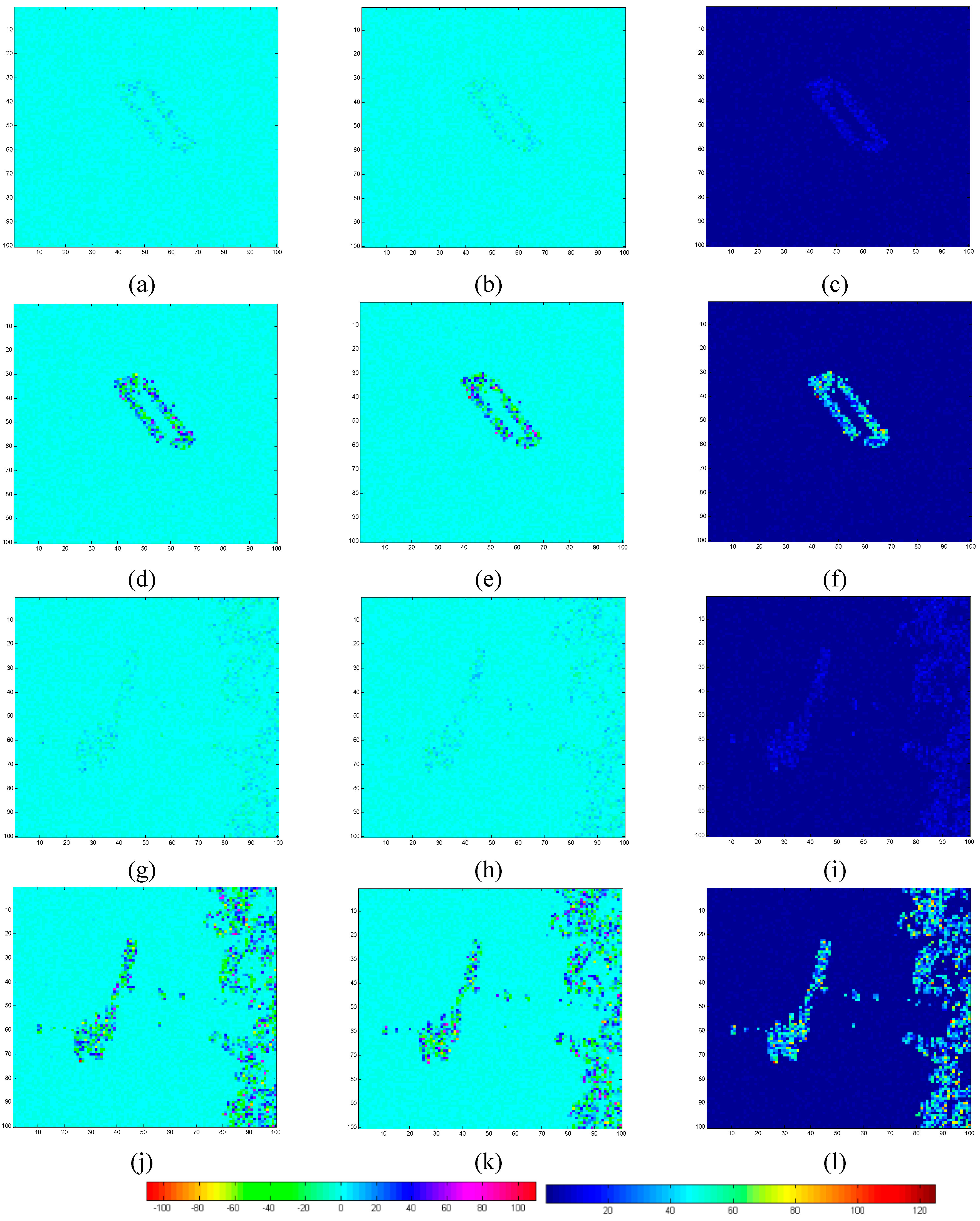
As examples, Figure 1 shows four simulated radar scenes with two sparsity levels (0.03 and 0.15), and two TBRs (25 and 900). The two sparsity levels represent extremely and moderately sparse scenes, respectively, while the two TBRs indicate small and large reflectivity differences between targets and background, respectively. Each scene is shown by a row of three sub-figures: real, imaginary and amplitude, from left to right. The first (Figure 1a–c) the second (Figure 1d–f) rows are for extremely sparse scenes of low and high TBRs, respectively, while the third (Figure 1g–i) and fourth (Figure 1j–l) rows are for moderately sparse scene of low and high TBRs, respectively. Clearly, targets of interest will be harder to detect from scenes of low TBRs than from those of high TBRs, meaning that we would need more sampled data to form images of acceptable detectability for the former than for the latter.

Figure 1. (a–c) real component, imaginary component and amplitude images of a scene of sparsity = 0.03 and TBR = 25, respectively; (d–f) real component, imaginary component and amplitude images of a scene of sparsity = 0.03 and TBR = 900, respectively; (g–i) real component, imaginary component and amplitude images of a scene of sparsity = 0.15 and TBR = 25, respectively; (j–l) real component, imaginary component and amplitude images of a scene of sparsity = 0.15 and TBR = 900, respectively.

Figure 1. (a–c) real component, imaginary component and amplitude images of a scene of sparsity = 0.03 and TBR = 25, respectively; (d–f) real component, imaginary component and amplitude images of a scene of sparsity = 0.03 and TBR = 900, respectively; (g–i) real component, imaginary component and amplitude images of a scene of sparsity = 0.15 and TBR = 25, respectively; (j–l) real component, imaginary component and amplitude images of a scene of sparsity = 0.15 and TBR = 900, respectively.

For simulating noisy echo data, we need also to specify radar parameters, as indicated in Equation (3). They are as follows: slant range of scene center 10 km, transmitted pulse duration 1 μs, range FM rate 150 MHz/μs, signal bandwidth 150 MHz, range sampling rate 164.829 MHz, effective radar velocity 7608 m/s, radar center frequency 9.650 GHz, radar wavelength 0.031 m, azimuth FM rate 372372 Hz/s, synthetic aperture length 57.383 m, target exposure time 0.007543 s, antenna length 4.8 m, Doppler bandwidth 2808.620 Hz, azimuth sampling rate 2920.018 Hz. For convenience, these parameter values are listed in Table 1. They were used to generate a convolution kernel matrix A_full with a dimensionality of 10,000 by 10,000 at full rank.

To generate a set of realized noise N and echo data Y, we set up a series of S(C)NR (equally spaced in the interval −5 ~ 20 dB, step = 0. 253 dB, indicating a total of 100 noise levels), and undersampling ratios (equally spaced in the interval 0.01 ~ 1, step = 0.01, a total of 100 undersampling ratios), to reflect the noise levels and compression ratios of Y, respectively. For each set of simulated X and specified sampling S(C)NR, we generated the corresponding set of N and Y. Noiseless linear measurements Y₀ were generated by pre-multiplying the signal X with a compressive sampling matrix A_sub, which consists of a number of randomly drawn rows from the measurement matrix A (A_full to be exact); the number of rows m for A_sub reflects the undersampling ratio being considered. Although, for any undersampling ratios less than 1, the possible combinations of rows for Asub are $C_m^n$ (the number of combinations of n distinct objects taken m at a time), we only pick up consecutive rows from A_full, starting from the first row, resulting in sets of A_sub’s (to reflect the undersampling ratios specified), which will be more conservative in terms of informational efficiency. The simulated measurements Y₀ were corrupted with additive Gaussian noise vectors N (with a length commensurate with those of Y₀’s), whose powers are restricted to the given S(C)NR level, to simulate noisy and undersampled echo data Y.

Table 1. Hypothetic radar parameters.

Parameter Name		Symbol	Value	Units
Range parameters	Slant range of scene center	$R_0$	10	km
	Transmitted pulse duration	Tr	1	μs
	Range FM rate	Kr	150	MHz/us
	Signal bandwidth	Br	150	MHz
	Range sampling rate	Fr	164.829	MHz
Azimuth parameters	Effective radar velocity	Vr	7608	m/s
	Radar center frequency	f0	9.650	GHz
	Radar wavelength	λ	0.031	m
	Azimuth FM rate	Ka	372372	Hz/s
	Synthetic aperture length	Ls	57.383	m
	Target exposure time	Ta	0.007543	sec
	Antenna length	La	4.8	m
	Doppler bandwidth	Ba	2808.620	Hz
	Azimuth sampling rate (PRF)	Fa	2920.018	Hz

Table 1. Hypothetic radar parameters.

Parameter Name		Symbol	Value	Units
Range parameters	Slant range of scene center	$R_0$	10	km
	Transmitted pulse duration	Tr	1	μs
	Range FM rate	Kr	150	MHz/us
	Signal bandwidth	Br	150	MHz
	Range sampling rate	Fr	164.829	MHz
Azimuth parameters	Effective radar velocity	Vr	7608	m/s
	Radar center frequency	f0	9.650	GHz
	Radar wavelength	λ	0.031	m
	Azimuth FM rate	Ka	372372	Hz/s
	Synthetic aperture length	Ls	57.383	m
	Target exposure time	Ta	0.007543	sec
	Antenna length	La	4.8	m
	Doppler bandwidth	Ba	2808.620	Hz
	Azimuth sampling rate (PRF)	Fa	2920.018	Hz

As mentioned previously, informational analysis was performed based on simulated radar scenes X and echo measurements Y. We used the simulated scene and echo data to perform information-theoretic graphing of R_X(D), using Equation (14), and trans-information $I{(X;Y|A)}_{ub}$ using (20) and $I{(X_1;Y|A)}_{ub}$ using (25). We applied inequalities in (26) and (27) to determine minimal undersampling ratios for signal reconstruction given certain values of sparsity, TBRs, noise, and distortion D. These are explained one by one in the following sub-sections

3.2. Visualization of Scene Rate-Distortion and Echo Data’s Trans-information

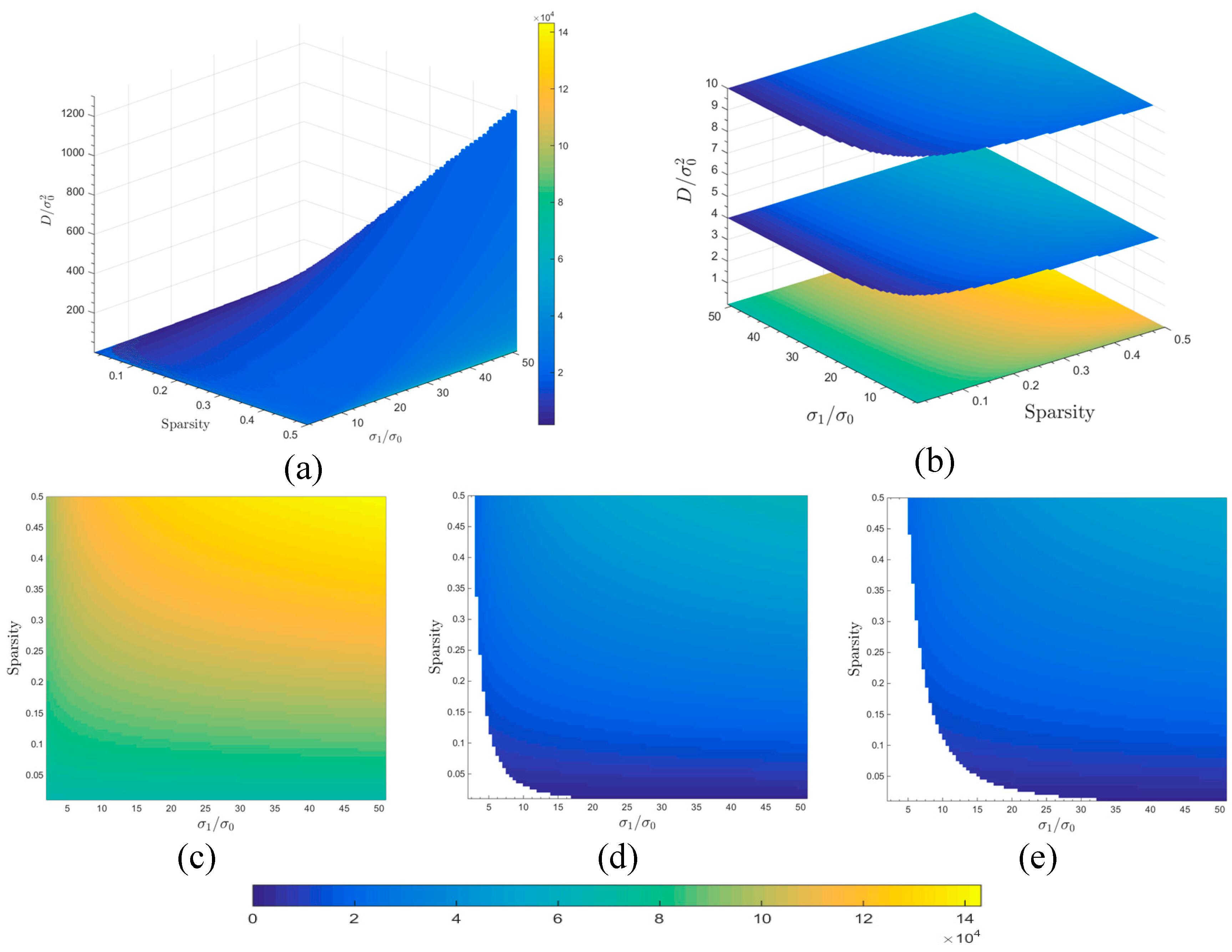
For visualizing rate-distortion trade-offs, we compute required minimum information rates for a range of distortion levels. We specified distortion levels D in the interval from 0.01 to 1300 (times ${\sigma }_0^2$, which was set to 1.0 though); the end value of 1300 is the maximum value beyond which the distortion is theoretically achievable for any specified combination of sparsity, TBRs, S(C)NRs and undersampling ratios. Three values of D (0.01, 4, and 10, all relative to ${\sigma }_0^2$) were selected to represent high, medium high, and moderate accuracy levels, respectively, although many more levels of distortion can be specified in principle.

A simulated compressible scene X corresponds to a specific sparsity and a particular TBR. Given a distortion D, the rate distortion (n*R(D)) of X can be calculated using Equation (14). The case of an extremely large value of TBR (e.g., TBR = 50²) refers to strictly sparse scenes, and their rate distortion can be approximated by (15).

Figure 2. (a) Visualization of rate-distortion relations in the three-dimensional space framed by sparsity, TBRs (actually shown as ${\sigma }_1/{\sigma }_0$ to reduce the range of values), and distortion; (b) three slice images representing varying rate distortion characteristics as related to different sparsities and TBRs when setting D = 0.01, 4 and 10, respectively (from bottom to top); (c–e) two-dimensional graphs showing rate-distortion relations for distortion D = 0.01, 4 and 10, respectively (all D values are relative to ${\sigma }_0^2$).

Figure 2. (a) Visualization of rate-distortion relations in the three-dimensional space framed by sparsity, TBRs (actually shown as ${\sigma }_1/{\sigma }_0$ to reduce the range of values), and distortion; (b) three slice images representing varying rate distortion characteristics as related to different sparsities and TBRs when setting D = 0.01, 4 and 10, respectively (from bottom to top); (c–e) two-dimensional graphs showing rate-distortion relations for distortion D = 0.01, 4 and 10, respectively (all D values are relative to ${\sigma }_0^2$).

Figure 2a–e shows rate distortion characteristics of various simulated scenes X, which have different sparsities and TBRs, in relation to distortion D. In particular, Figure 2a indicates that rate distortion in relation to a distortion D is meaningful only within a certain region of scene sparsities and TBRs by virtue of its achievable regions, although the inner part of the 3-dimensional graphics is not visible. To see some of its inner information “landscape” implied in Figure 2a, we display slices of rate-distortion relations corresponding to distortion values of 0.01, 4, and 10, respectively, in the order from bottom to top, as shown in Figure 2b. For more clarity in graphing, Figure 2c–e highlights the slices where distortion D is fixed at 0.01, 4, and 10, respectively. Obviously, information rates required for lossy compression (or approximate reconstruction) grow with decreased distortion thresholds, and for a fixed distortion D the required information rates increase with increasing sparsity and TBRs, though the relationships are not linear.

The quantities of mutual information $I{(X;Y|A)}_{ub}$ and $I{(X_1;Y|A)}_{ub}$ measure the amounts of trans-information conveyed by measurements Y about the scene X and the targets of interest X₁, respectively. The former can be evaluated using Equation (20), while latter can be assessed using Equation (25), given differing sampling specifications (i.e., number of measurements and noise levels) and scene characteristics (i.e., sparsities and TBRs). 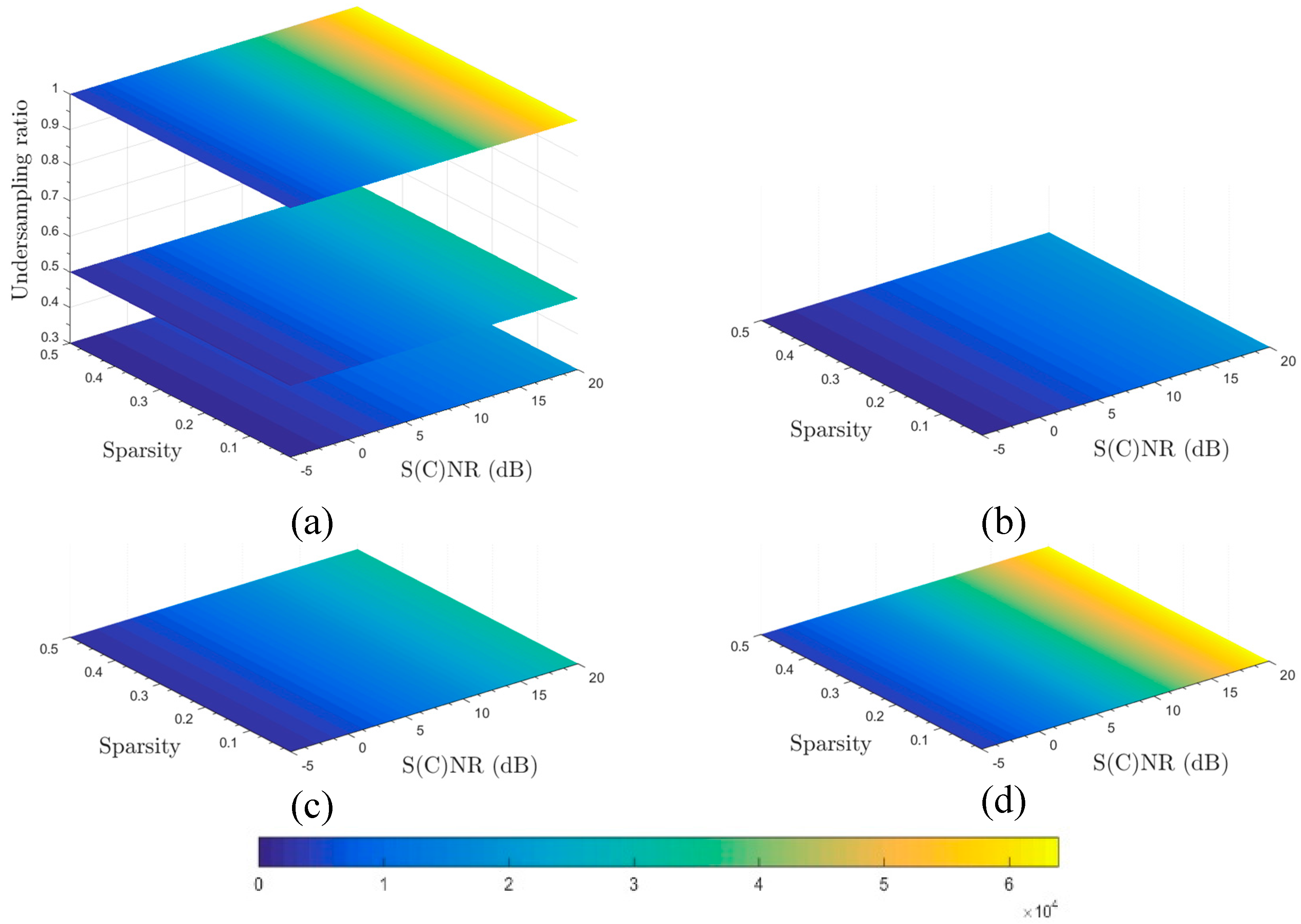Figure 3 and Figure 4 show the upper bounds of mutual information of echo data about X and X₁, respectively, in relation to undersampling ratios, sparsity and TBRs (for $I{(X_1;Y|A)}_{ub}$), and S(C)NR.

Figure 3. (a) slice images showing mutual information conveyed by echo data about the underlying scene with three undersampling ratios; (b–d) slice images for undersampling ratios of 0.3, 0.5, and 1.0, respectively.

Figure 3. (a) slice images showing mutual information conveyed by echo data about the underlying scene with three undersampling ratios; (b–d) slice images for undersampling ratios of 0.3, 0.5, and 1.0, respectively.

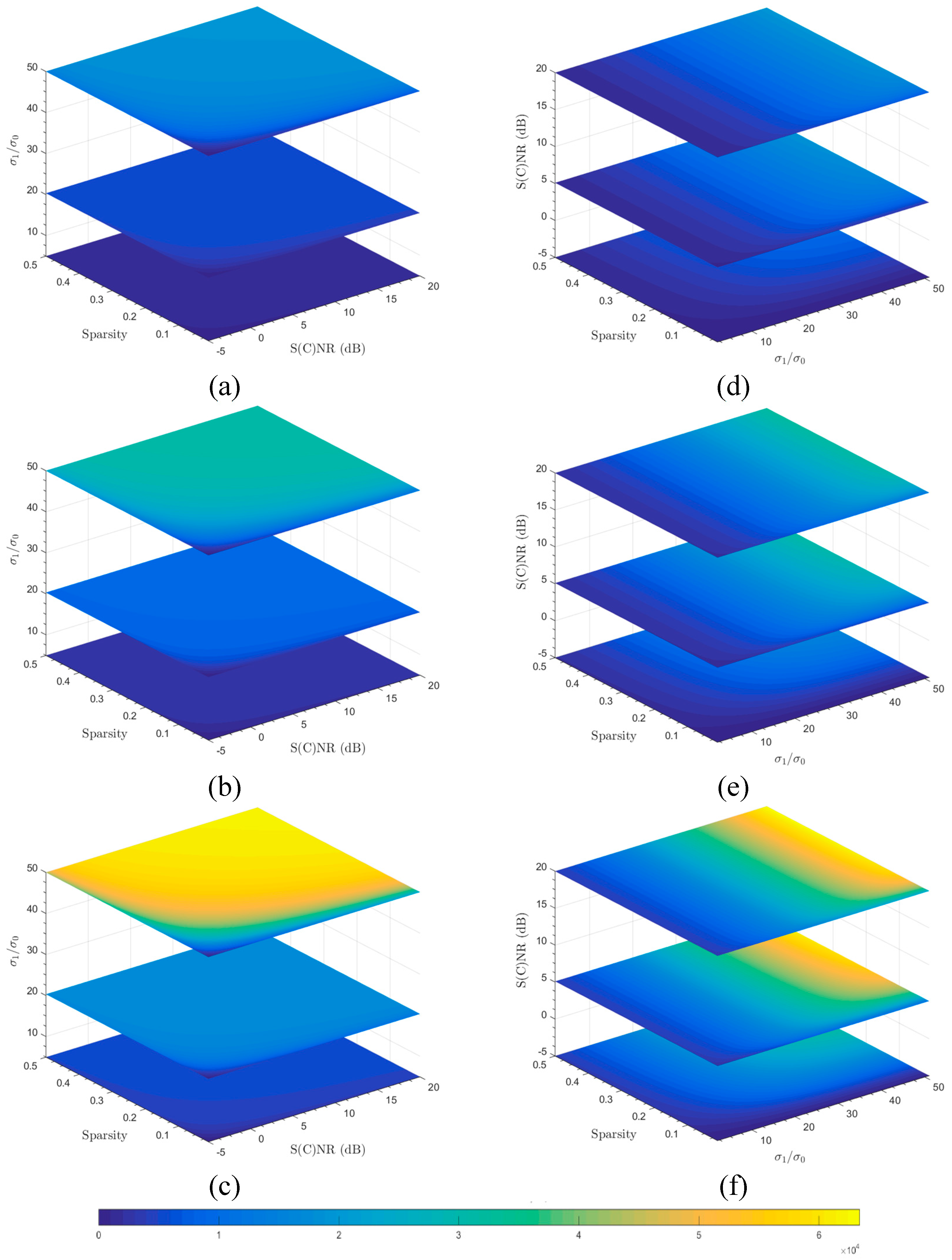
Figure 4. Slice images representing varying mutual information conveyed by echo data about the targets of interest under different undersampling ratios, sparsity, TBR (actually ${\sigma }_1/{\sigma }_0$), and S(C)NR: (a–c) undersampling ratios = 30% , 50% and 100%, respectively, and all with TBRs (in vertical axes) of 25, 400 and 2500 (i.e., 5, 20 and 50 in terms of ratios of square root TBRs as shown in the Figures) from bottom up; (d–f) 30% , 50% and 100% undersampling ratios, respectively, and all with S(C)NR (in vertical axes) of −5, 5 and 20 dB.

Figure 4. Slice images representing varying mutual information conveyed by echo data about the targets of interest under different undersampling ratios, sparsity, TBR (actually ${\sigma }_1/{\sigma }_0$), and S(C)NR: (a–c) undersampling ratios = 30% , 50% and 100%, respectively, and all with TBRs (in vertical axes) of 25, 400 and 2500 (i.e., 5, 20 and 50 in terms of ratios of square root TBRs as shown in the Figures) from bottom up; (d–f) 30% , 50% and 100% undersampling ratios, respectively, and all with S(C)NR (in vertical axes) of −5, 5 and 20 dB.

As shown in Figure 3a, three images are created from slicing the informational cube, which can not be completely depicted here, in the three-dimensional space framed by sparsity, S(C)NR, and undersampling ratios, at three undersampling ratios: 0.3, 0.5, and 1.0 (in bottom-up sequence). For enhanced visualization, the three slices of images depicted in Figure 3a are shown in Figure 3b–d, respectively, in the two-dimensional space of sparsity and S(C)NR. Unsurprisingly, trans-information increases with increasing undersampling ratios. For a fixed undersampling ratio, trans-information increases with increasing S(C)NR, though the increase in trans-information is not related to sparsity at a fixed S(C)NR, as is apparent in Equation (20) for computing $I{(X;Y|A)}_{ub}$.

Figure 4a–c shows slice images representing varying mutual information conveyed by echo data about the targets of interest under different sparsities, TBRs, and S(C)NR with undersampling ratios of 30% , 50%, and 100%, respectively. In Figure 4a–c, TBRs are actually shown as ${\sigma }_1/{\sigma }_0$ and measure 5, 20 and 50 from bottom up in the vertical axes. To visualize the other aspects of trans-information $I{(X_1;Y|A)}_{ub}$ landscapes, Figure 4d–f shows slice images of $I{(X_1;Y|A)}_{ub}$ under different sparsities, S(C)NR, and TBRs (${\sigma }_1/{\sigma }_0$), again with undersampling ratios of 30% , 50%, and 100%, respectively. In Figure 4d–f, S(C)NR are shown in vertical axes and measure −5, 5, and 20 dB from the bottom up.

In comparison, trans-information quantities shown in Figure 4a–c tend to be more conservative than that in Figure 3a–c, assuming the same undersampling ratios, sparsities, and S(C)NRs, especially with lower TBRs. The graphics shown in Figure 3a–c and Figure 4d–f are not directly comparable. Thus, we will not elaborate on this here.

3.3. Undersampling Ratios in Graphics

The minimal undersampling ratios can be determined through evaluating the information-theoretic inequality in (26). This can be done by numerically solving an equation between the mutual information $I{(X;Y|A)}_{ub}$ and rate distortion implied in (26). These ratios are conditional to the simulated measurement matrix A, and evaluated for a given scene with a certain sparsity and noise level as indicated by S(C)NR.

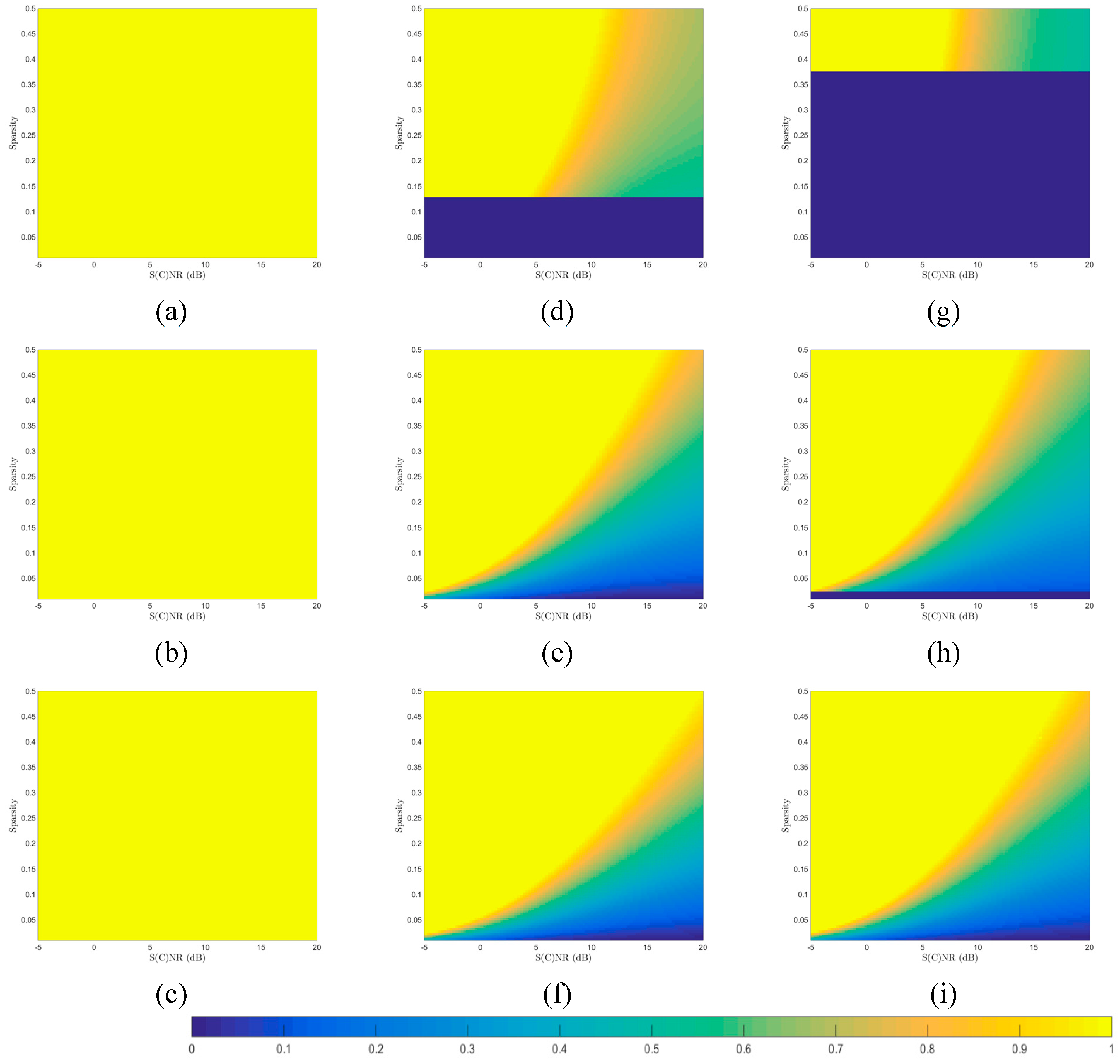
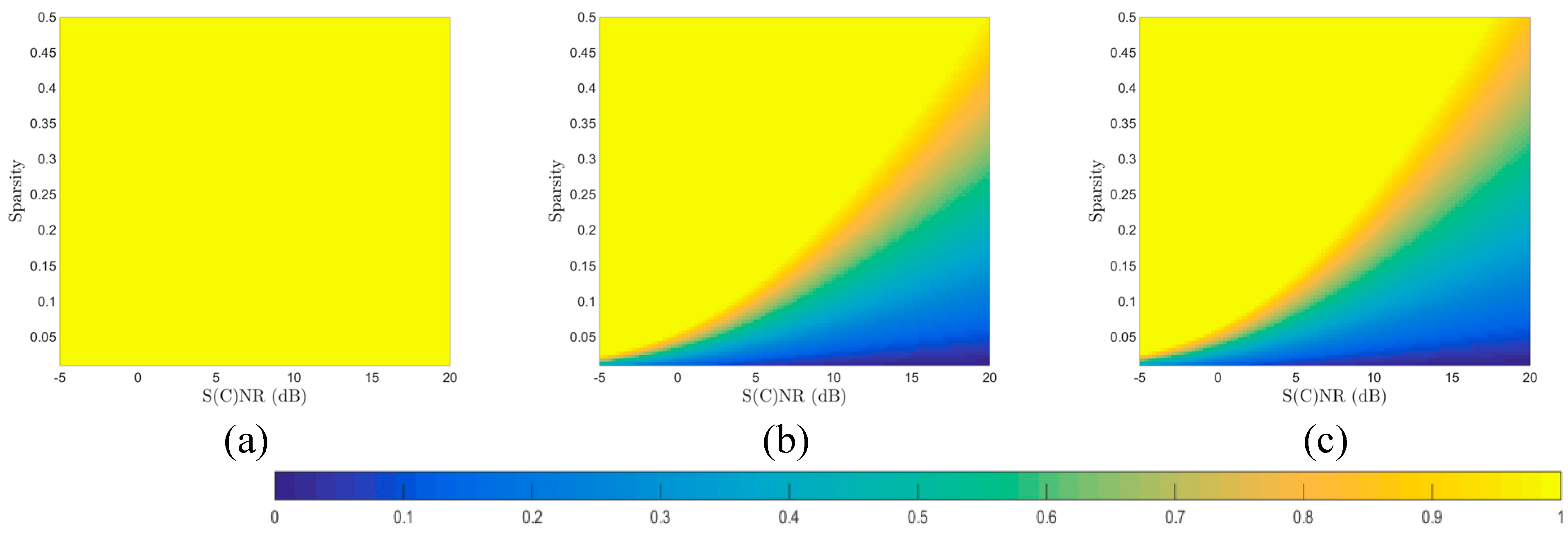
Figure 5a–c shows the images indicating minimal (i.e., necessary) undersampling ratios in relation to scene sparsity and per-sample S(C)NR, given MSE distortion levels D of 0.01, 4, and 10, respectively. As previously, distortion levels D are relative to ${\sigma }_0^2$. Clearly, with more relaxed or greater distortion thresholds, the undersampling ratios required will be reduced, given the same values of scene sparsity and per-sample S(C)NR.

Figure 5. Minimal under-sampling ratios in relation to signal sparsity and per-sample S(C)NR, given distortion level of 0.01 (a), 4 (b), and 10 (c), respectively.

Figure 5. Minimal under-sampling ratios in relation to signal sparsity and per-sample S(C)NR, given distortion level of 0.01 (a), 4 (b), and 10 (c), respectively.

Similarly, the minimal undersampling ratios for target detection in a given scene and with noise level can be determined through evaluating the information-theoretic inequality in (27). Again, this can be done by numerically solving an equation between the mutual information $I{(X_1;Y|A)}_{ub}$ and rate distortion implied in (27). These ratios are also conditional to the simulated measurement matrix A.

As rate distortion is, by definition, distortion-dependent, we show selectively (according to D thresholds) some of the phase diagrams, which map the regions where sampling conditions are satisfied, as in Figure 5. The phase diagrams in Figure 6 show required minimal undersampling ratios in relation to scene sparsity, TBRs, and per-sample S(C)NR.

Figure 6. Minimal undersampling ratios in relation to signal sparsity and per-sample S(C)NR, given distortion level of 0.01 (a–c), 4 (d–f), and 10 (g–i), and TBRs of 25 (a,d,g), 400 (b,e,h), and 2500 (c,f,i); all MSE distortion levels are relative to pre-set ${\sigma }_0^2$.

Figure 6. Minimal undersampling ratios in relation to signal sparsity and per-sample S(C)NR, given distortion level of 0.01 (a–c), 4 (d–f), and 10 (g–i), and TBRs of 25 (a,d,g), 400 (b,e,h), and 2500 (c,f,i); all MSE distortion levels are relative to pre-set ${\sigma }_0^2$.

To assist interpretation of the results, these diagrams are organized in row and column groups. The row grouping is based on TBRs (actually ${\sigma }_1/{\sigma }_0$): 5 (Figure 6a,d,g), 20 (Figure 6b,e,h), and 50 (Figure 6c,f,i). The column grouping is based on MSE distortion levels: 4 (Figure 6a–c), 100 (Figure 6d–f), and 400 (Figure 6g–i), where all MSE distortion levels are relative to ${\sigma }_0^2$. Similar to the phase diagrams in Figure 5, greater distortion thresholds lead to smaller necessary undersampling ratios, given the same values of scene sparsities, TBRs and per-sample S(C)NRs. With increasing TBRs, necessary under-sampling ratios will be decreased, while all other settings are kept the same. An important link can be made of the similarity between phase diagrams shown in Figure 5a–c and those in Figure 6c,f,i, as the former represent the limiting cases of those in Figure 6, when TBRs become sufficiently large (e.g., ${\sigma }_1/{\sigma }_0$ = 50).

Note that the blue blocks in Figure 6d,g,h indicate that we would not need to acquire any samples for approximate reconstruction of the underlying scenes due to relaxed distortion thresholds, small sparsity, and low TBRs. This means that there is little information in such kind of scenes in the first place so that no sampling is required for reconstruction of X and X₁ with distortion thresholds indicated by D. Here, approximate reconstruction means that the underlying scene is reconstructed, with targets of interest properly detected and estimated, up to given distortion thresholds.

The derived undersampling ratios are necessary conditions, meaning that scene reconstruction would not be possible without incurring distortion larger than the prescribed thresholds if the numbers of measurements are less than what is indicated by the undersampling ratios. Even if the sampling necessary conditions are satisfied, there is no guarantee that such properly undersampled data will enable scene reconstruction meeting the specified distortion criterion. The reasons are three-fold: (1) necessary conditions are not sufficient ones, (2) information-theoretically derived sampling necessities are theoretical and algorithm-independent while algorithms may incur extra expenses of sampling, and (3) sampling necessary conditions derived previously are meaningful on probabilistic terms, suggesting variabilities in trade-offs between sampling and distortion.

As mentioned previously, the results obtained with simulated data are conditional to the particular measurement matrix A set forth, as is also the case with Zhang and Yang [15]. In other words, our results are not invariant to measurement matrices and hence the radar transmitted waveforms and other relevant parameters employed in a CS system. This raises, for instance, the issue of how waveforms should be designed to maximize mutual information between Y and X, as discussed by Bell [22]. Clearly, the existing literature on related topics and the results obtained here in this paper should be integrated to push forward research on CS-radar informatics and sampling theorems. For instance, the informational quantities described in this paper in the context of CS-radar should be made to augment the existing predominantly statistical metrics for performance evaluation of radar systems. On the other hand, we should consider the aforementioned computational approaches to phase transitions to handle peculiar signal models, sampling matrices, reconstruction algorithms and performance evaluation criteria, which are otherwise difficult to analyze theoretically.

3.4. Discussion

In this sub-section, we discuss the results by first comparing undersampling ratios derived from information-theoretic analysis and those based on the restricted isometry property (RIP) in classical CS theory. We will also reflect on future developments in compressive radar imaging, focusing on compressible radar scene modeling and sparsity-enhancement in radar imaging.

CS sensing matrices and reconstruction algorithms function like encoders and decoders in the context of information theory, with the former seeking to preserve information content in the sparse signal while the latter aiming to be efficient and robust for recovering the original signal in presence of measurement noise. The so-called RIP is one of desirable properties that we would like CS sensing matrices to have so that the sensing matrices possess adequate level of efficiency in transferring information in the original signal. With a sensing matrix satisfying the RIP, various algorithms will be able to successfully recover sparse signals from noisy measurement, according to established RIP-based CS results [53]. The necessary numbers of measurements needed to achieve the RIP are studied widely in CS literature. Here, we mention one of such results originally reviewed by Davenport et al. [53]. Let A be an $m\times n$ matrix that satisfies the RIP of order 2 k with RIP constant $\delta \in$ (0, 0.5], where m and n represent the number of measurements Y and the length of signal vector X, respectively. Then, RIP requirements can be used to derive phase transition for a problem dimension {k, m, n} such that $m>ck\log (n/k)$ with $c\approx 0.28$ [53].

There exist a few major distinctions between information-theoretically determined undersampling ratios in this paper and RIP results. We highlight some of them in terms of the signal models, sensing matrices and reconstruction criteria concerned. First, sparse signals are usually described by just sparsity in RIP, while both sparsity and TBRs are accommodated in GMMs-based signal models in the paper. The two-component (i.e., target-clutter) GMMs employed therein were shown to have well supported the tasks of target detection against clutter interference in approximately sparse radar scenes. This represents a major strength and contribution of this paper.

Secondly, randomized sensing matrices such as those drawn from i.i.d. Gaussian distributions are preferred in RIP-based analysis for under-sampling ratios. Although deterministic sensing matrices can also be considered in CS literature through the concept of coherence [53] and its relationships with RIP, the derived under-sampling ratios are often unacceptably high. On the other hand, informational analysis performed in this paper was based on deterministic sensing matrices, which are common in compressive radar imaging. The information-theoretic limits on undersampling were shown to be related to l₂-norms of the sensing matrix rows, which are easier to analyze and optimize, as seen previously.

Thirdly, RIP-derived phase transition is mostly about exact or precise recovery [27], although relations between achievable minimum errors in signal recovery and RIP constants are confirmed in the literature [54]. In informational analysis reported in this paper, rate distortion was shown to be a valuable theoretic construct to analyze the trade-offs between information rates and distortion tolerance, as shown in Figure 2. Thus, the phase diagrams shown in Figure 5 and Figure 6 of the paper were distortion-specific. Furthermore, mutual information computed for a set of compressive measurements can be used as a quality measure for the images formed from under-sampled data, as discussed towards the end of Section 2. Clearly, the information-theoretic quantification about sampling-distortion trade-offs is particularly useful for compressive radar imaging where sampling efficiency, target detectability and imaging quality are important considerations.

Although GMMs were employed to model compressible radar scenes in this paper, we may well use other kinds of models for modeling complex-valued radar reflectivities if empirical evidence suggests so. For example, it was found that Laplace distributions are more suitable to model complex-valued images under wavelet transforms than Gaussian distributions, as shown in Xu et al. [13]. Further research is needed for balancing between model complexity (hence related computational cost) and precision in modeling. The mixture distribution models are versatile and worth exploring in applications. For instance, it is interesting to extend use of GMMs by modeling both sparse targets of interest and the clutter interference through their respective GMMs.

In this paper, complex-valued radar images were represented by real and imaginary parts. Since phase components are not sparse due to them being uniformly distributed in the interval of [−π, π], we often model and represent sparsity in radar images based on their amplitude components alone. However, the complex nature of original images and the mechanism of coherent radar imaging require treatment of both amplitude and phase [55], even if we need amplitude images only as the end results. Nevertheless, there remains the issue of optimum sparse representation and sparsity/feature-enhanced imaging algorithms for compressible radar scenes, as elaborated below.

We may enforce sparsity in amplitude alone in CS-based radar imaging by modifying objective functions for signal reconstruction. The so-called sparsity-enhanced methods for compressive radar imaging may be usefully explored, as described by [55]. The cost functional to minimize includes sparsity-enforcing weights on the vectors of amplitudes and their gradients, in addition to an l₂-norm on the differences between complex-valued measurements Y and reconstruction-induced projections AX. To avoid potential conflicting of these two kinds of constraints, we need to employ joint optimization of amplitudes and phases via alternating minimization of objective functions. One acts explicitly on amplitudes with initial estimation of phases, while the other on phases based on updated estimates of amplitudes. The joint optimization is done through an iterative process until convergence. This approach provides the capability to preserve and enhance multiple distinct features on different patches of the underlying scene. Nevertheless, the algorithms employed above are tailor-made, and a joint optimization strategy tends to be computationally more expensive than the algorithm adopted in this paper, as it is originally developed for real-valued signal processing and imaging.

4. Conclusions

This paper has presented an information-theoretic strategy, which is seen to be complementary to the classic CS theory, to describe, analyze and interpret information dynamics in compressive radar imaging. The undertaken informational analyses focused on compressibility of radar scenes and trans-information of radar measurements about the underlying scene and the targets of interest, respectively. The amount of information conveyed by compressive sampling about targets of interest against clutter is more conservative as a measure of trans-information than that about the scene as a whole. The formulas for estimating the former (i.e., trans-information regarding targets of interest in clutter) constitute a major thrust of innovation of this paper. Quantification of compressible radar scene’s rate-distortion and trans-information of compressive radar measurements facilitates determination of necessary undersampling ratios. The necessary undersampling ratios derived for scene reconstruction vs. target detection/estimation, within certain MSE distortion thresholds, are seen to differ greatly, with the latter being more contingent, given that it has to accommodate the task of detecting targets of interest against clutter interference, as target detection/estimation is dependent, additionally, on target-to-background variance ratios (TBRs). A simulated experiment illustrated theoretical derivations and their use through computer-generated graphics visualizing scene-sampling-distortion inter-relationships with an information-theoretic perspective. This work will also be constructive for CS-radar sampling design via undersampling ratios determination and performance evaluation by using trans-information as upper bounds on information content of reconstructed images. For instance, a specific radar imaging application with a particular scene and image distortion corresponds to a set of “points” over the information-theoretically generated graphics, and can thus be informed of its corresponding rate-distortion, trans-information and necessary under-sampling ratio. Moreover, the general framework proposed in this paper can be applied to other computational imaging applications that capitalize on CS principles and techniques.

The results derived regarding informational analysis and necessary sampling rates for compressible radar scene reconstruction from undersampled echo data can be extended to two scenarios. One concerns discrete support recovery only, which requires less amount of sampling obviously, while the other about conditions for exact reconstruction as opposed to approximate reconstruction, as presented here in this paper, although this is not elaborated here in this paper. Future research should, hopefully, also address issues related to real applications, as it is important to showcase CS theorems and their practicality in radar imaging and other fields.