Radial Wavelet Neural Network with a Novel Self-Creating Disk-Cell-Splitting Algorithm for License Plate Character Recognition

Abstract

In this paper, a novel self-creating disk-cell-splitting (SCDCS) algorithm is proposed for training the radial wavelet neural network (RWNN) model. Combining with the least square (LS) method which determines the linear weight coefficients, SCDCS can create neurons adaptively on a disk according to the distribution of input data and learning goals. As a result, a disk map is made for input data as well as a RWNN model with proper architecture and parameters can be decided for the recognition task. The proposed SCDCS-LS based RWNN model is employed for the recognition of license plate characters. Compared to the classical radial-basis-function (RBF) network with K-means clustering and LS, the proposed model can make a better recognition performance even with fewer neurons.

1. Introduction

Nowadays automatic license plate recognition (ALPR) plays an important role in many automated transport systems such as road traffic monitoring, automatic payment of tolls on highways or bridges and parking lots access control. In general, four major steps are comprised in these recognition systems, namely locating of car plate regions, correction of slant plates, segmentation of characters from the plate regions and recognition of car plate characters. Many researchers have been making great efforts on ALPR systems. In [1], a recognition system of China-style license plate is proposed, which adopt the color and vein characteristics locating plate, mathematical morphology and Radon transformation correcting the slant plate and BP neural network recognizing characters. In [2], a distributed genetic algorithm is used to extract license plates from vehicle images. In [3], a least-square-based skew detection method is proposed for skew correction and template matching combining with Bayes methods are used to get robust recognition rates in the recognition system. In [4], the morphological method is used to detect the candidates of the Macao license plate region and a template matching combining a post-process is used to recognition characters. In [5], the self-organizing map (SOM) algorithm is used to make the slant correction of plates and a hybrid algorithm cascading two steps of template matching is utilized to recognize Chinese characters segmented from the license plates, which is based on the connected region feature and standard deviation feature extracted from sample corresponding to each template. Some other methods can also been found in [6–10].

In this study, the character recognition step which belongs to the pattern recognition field is considered. As to the recognition of license plate character, there are two important aspects: feature extraction and classification method. There have been a lot of methods on the feature extraction of characters, which are based on the projections, strokes, counters, skeletons, pixels number in grids, Zernike moment and wavelet moment etc. All these features can be used alone or associatively. The most commonly used classification methods are template matching [3–5,9] and neural network [1,7,8,10]. The former is based on the difference between sample and template, and the latter is based on the generalization ability of the network.

Neural network approaches can be considered as “black-box” methods which possess the capability of learning from examples with both linear and nonlinear relationships between the input and output signals. After years of development, neural network has been a popular tool for time-series prediction [11,12], feature extraction [13,14], pattern recognition [15,16], and classification [17,18]. Due to the ability of wavelet transformation for revealing the property of function in localize region, different types of wavelet neural network (WNN) which combine wavelets with neural networks have been proposed [19,20]. In WNN, the wavelets were introduced as activation functions of the hidden neurons in traditional feedforward neural networks with a linear output neuron. As to the WNN with multidimensional input vectors, multidimensional wavelets must employed in the hidden neurons. There are two commonly used approaches for representing multidimensional wavelets [21]. First one is to generate separable wavelets by the tensor product of several 1-D wavelet functions [19]. Another popular scheme is to choose the wavelets to be some radial functions in which the Euclidian norms of the input variables are used as the inputs of single-dimensional wavelets [21–23]. In this paper, the radial wavelet neural network (RWNN) is used as the means for plate character data classification.

It is well-known that selecting an appropriate number of hidden neurons is crucial for good performance and meanwhile the first task determining the architecture of the feedforward neural networks. The same is true of radial wavelet neural network, which is based on the Euclidean distance. In this view, a novel self-creating and self-organizing algorithm is proposed to determine the number of hidden neurons. Based on the idea of SOM which can produce an ordered topology map of input dada in a low dimensional space, the proposed self-creating disk-cell-splitting algorithm can create neurons adaptively on a disk according to the distribution of input data and learning goals, which accordingly produces a RWNN with proper structure and parameters for the recognition task. In addition, the splitting method endows weights of new generated neurons through circle neighbor strategy and maintains the weights of non-splitting neurons which can ensure a faster convergence process.

The content of this paper is organized as follows. In Section 2, a brief introduction of radial wavelet neural network is given. Followed by a review of self-organizing map algorithm, the detailed self-creating disk-cell-splitting (SCDCS) algorithm combining the least square (LS) method which used for RWNN is described in Section 3. In Section 4, two simulation examples: recognition of English letters and recognition of numbers or English letters are implemented by SCDCS-LS based RWNN model as well as the classical K-means-LS based RBF model. The comparison results are presented to demonstrate the superior ability of our proposed model. Finally, some conclusions are drawn in the last section.

2. Radial Wavelet Neural Network (RWNN)

Wavelets in the following form:

$${\psi }_{a,b}=|a{|}^{-1/2}\psi (\frac{x-b}{a}),a,b\in R,a\ne 0$$

(1)

are a family of functions generated from one single function $\psi (x)$ by the operation of dilation and translation. $\psi (x)\in L^2(R)$ is called a mother wavelet function that satisfies the admissibility condition:

$$C_{\psi }={\displaystyle {\int }_0^{+\infty }\frac{|\widehat{\psi }(\omega ){|}^2}{\omega }d\omega }<+\infty$$

(2)

where $\widehat{\psi }(\omega )$ is the Fourier transform of $\psi (x)$ [24,25].

Grossmann [26] proved that any function $f(x)$ in $L^2(R)$ can be represented by Equation (3):

$$f(x)=\frac{1}{C_{\psi }}{\displaystyle \iint Wf(a,b)|a{|}^{-1/2}\psi (\frac{x-b}{a})}\frac{1}{a^2}dadb$$

(3)

where $Wf(a,b)$ given by

$$Wf(a,b)=|a{|}^{-1/2}{\displaystyle {\int }_{-\infty }^{+\infty }\psi (\frac{x-b}{a})f(x)dx}$$

(4)

is the continuous wavelet transform of f (x).

Superior to conventional Fourier transform, the wavelet transform (WT) in its continuous form provides a flexible time-frequency window, which narrows when observing high frequency phenomena and widens when analyzing low frequency behavior. Thus, time resolution becomes arbitrarily good at high frequencies, while the frequency resolution becomes arbitrarily good at low frequencies. This kind of analysis is suitable for signals composed of high frequency components with short duration and low frequency components with long duration, which is often the case in practical situations.

Inspired by the wavelet decomposition of $f(x)\in L^2(R)$ in Equation (3) and a single hidden layer network model, Zhang and Benveniste in [19] had developed a new neural network model, namely, wavelet neural network (WNN) which adopts the wavelets called also wavelons as the activation functions. The simple mono-dimensional input structure is represented by the following expression (5).

$$y(x)={\displaystyle \sum _{k=1}^{N_w}{w}_k\psi (\frac{x-b_k}{d_k})}+\overline{y}$$

(5)

The addition of the $\overline{y}$ value is to deal with function whose mean is nonzero. In a wavelet network, all parameters $w_k$ (connecting parameter), $\overline{y}$ (bias term), $d_k$ (dilation parameter), $b_k$ (translation parameter) are adjustable, providing certainly more flexibility to derive different network structures.

To deal with multidimensional input vectors, the multidimensional wavelet activation functions must be adopted in the network. One of the typical alternative networks is the radial wavelet network (RWN) introduce by Zhang in [22]. 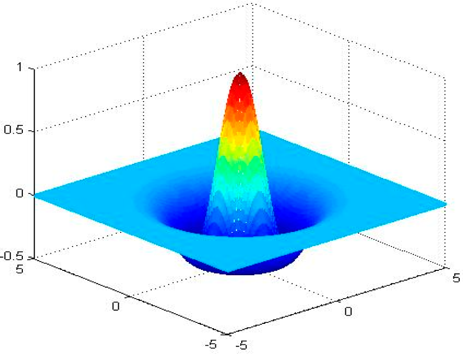A wavelet function $\Psi (\mathbf{x})$ is radial if it has the following form: $\Psi (\mathbf{x})=\psi (\Vert \mathbf{x}\Vert )$, where $\Vert \mathbf{x}\Vert ={({\mathbf{x}}^{\mathrm{T}}\mathbf{x})}^{1/2}$ and $\psi$ is a mono-variable function. In this paper, translated and dilated version of the Mexican Hat wavelet function is used, which is given by the following equation:

$${\Psi }_k(\mathbf{x})=(1-\frac{{\Vert \mathbf{x}-{\mathbf{b}}_k\Vert }^2}{d_k{}^2})\exp (-\frac{{\Vert \mathbf{x}-{\mathbf{b}}_k\Vert }^2}{2d_k{}^2})$$

(6)

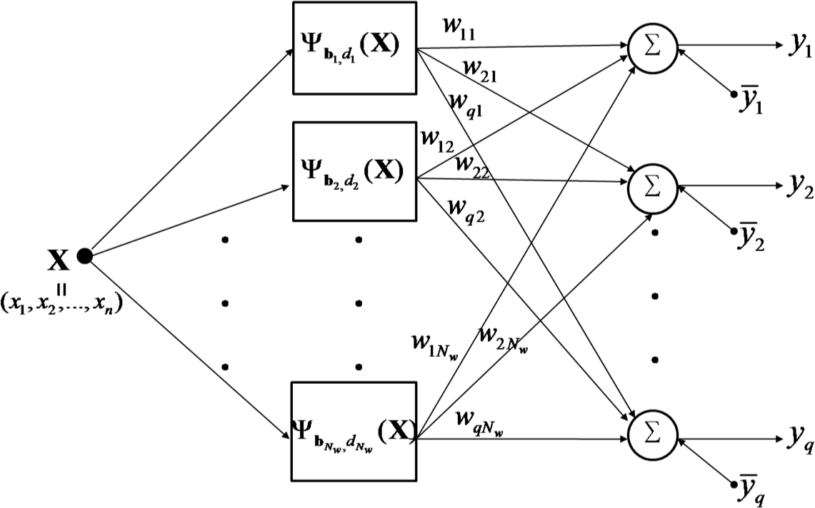
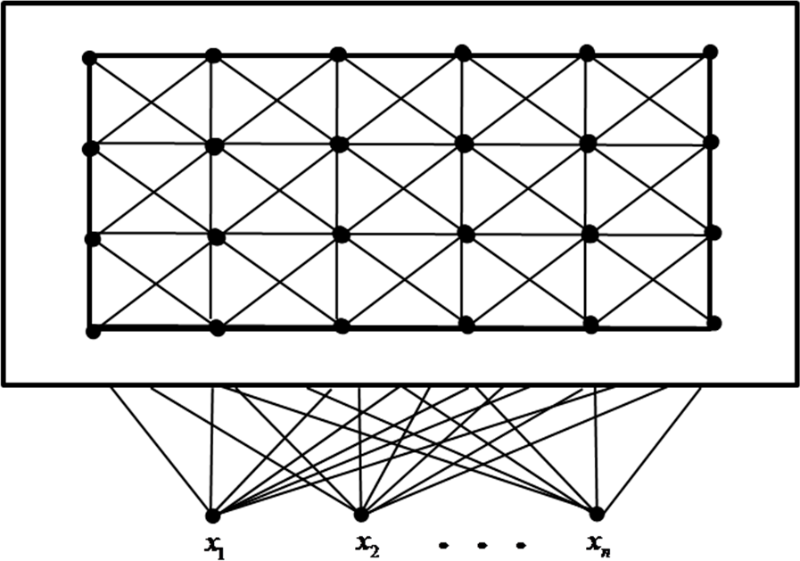
where ${\mathbf{b}}_k$ is the translation parameter with dimension identical to input record $\mathbf{x}$, $d_k$ is the scalar dilation parameter. A 2-D radial Mexican Hat wavelet function is drawn in Figure 1. Figure 2 shows the architecture of a RWNN, whose output neurons produce linear combination of the outputs of hidden wavelons and bias terms by the following equation:

$$y_p(\mathbf{X})={\displaystyle \sum _{k=1}^{N_w}{w}_{pk}{\Psi }_k(\mathbf{X})}+{\overline{y}}_p,p=1,\dots ,q$$

(7)

where N_w and q are the numbers of hidden and output neurons respectively.

3. Self-Creating Disk-Cell-Splitting (SCDCS) and Least Square (LS) Method Based RWNN

The parameters learning strategy of RWNN is different for the hidden layer and output layer as classical radial traditional radial-basis-function (RBF) network [27]. For finding the weights between the hidden and output layer, a linear optimization strategy—LS method is used in RWNN. While for the translation parameters of radial wavelets as well as the number of neurons in the hidden layer, a novel self-organizing type SCDCS algorithm is employed. The SCDCS-LS algorithm is based on the competitive learning of SOM, but the map is organized on a disk instead of a rectangular, and the mapping scale is self-creating by the input data and learning goals other than pre-determined. In this section, a brief review of SOM is presented firstly. After that the SCDCS-LS algorithm is detailed described.

3.1. Self-Organizing Map

SOM is a type of artificial neural network that is trained using unsupervised learning to produce a low-dimensional (typically two-dimensional), discretized representation of the input space of the training samples, and called a map. The model was first described as an artificial neural network by Teuvo Kohonen [28], and is sometimes called a Kohonen map. Figure 3 shows a Kohonen network connected to the input layer representing a n-dimensional vector.

The goal of learning in the self-organizing map is to cause different parts of the network to respond similarly to certain input patterns. This is partly motivated by how visual, auditory or other sensory information is handled in separate parts of the cerebral cortex in the human brain.

The training algorithm utilizes competitive learning. Detailed approach is as follows.

• Randomize the map’s nodes’ weight vectors W_v s.
• Grab an input vector X.
• Traverse each node in the map.

  • (i) Use Euclidean distance formula to find similarity between the input vector and the map’s node’s weight vector.
  • (ii) Track the node that produces the smallest distance (this node is the best matching unit, BMU).
• Update the nodes in the neighborhood of BMU by pulling them closer to the input vector as

  $${\mathbf{W}}_v(t+1)={\mathbf{W}}_v(t)+\theta (v,t)\alpha (t)(\mathbf{X}(t)-{\mathbf{W}}_v(t))$$

  (8)

  Here $\alpha (t)$ is a monotonically decreasing learning coefficient. The neighborhood function $\theta (v,t)$, usually takes Gaussian function form, depends on the lattice distance between the BMU and neuron v, and shrinks with time.
• Increase t and repeat from Step 2 while $t<\lambda$, where λ is the limit on time iteration.

3.2. SCDCS-LS Algorithm for RWNN

The main drawback of the conventional SOM is that one must predefine the map structure and the map size before commencement of the training process. This disadvantage is more obvious when the output neurons of one SOM are used as the hidden neurons of RWNN for clustering input data. Many trial tests may be required to find an appropriate number of hidden neurons, and re-clustering must be done when new neurons are added to the hidden layer. The proposed self-creating disk-cell-splitting algorithm is based on the competitive learning of SOM, but the map is organized on a disk instead of a rectangular, and the mapping scale is self-creating by the input data and learning goals. Moreover, the algorithm can effectively use the trained centers when new neurons are born, which makes the clustering process more efficiently.

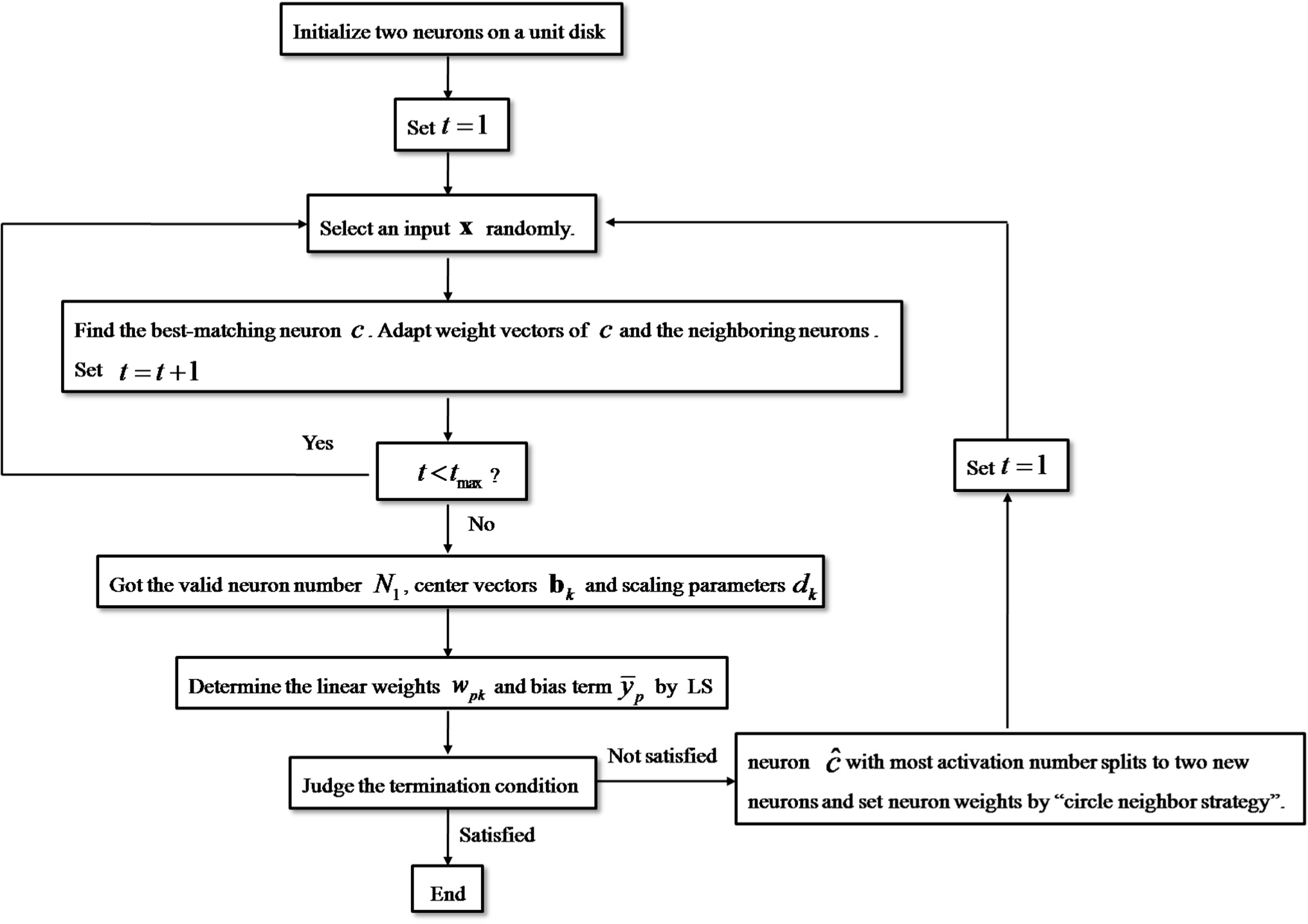
Figure 4 shows the flowchart of SCDCS-LS algorithm for RWNN. The executing steps can be divided into five modules expressed as follows.

• ♦ The second module: Competitive learning

  • 1. Select an input x randomly from input samples and find the best-matching neuron c in neurons such that $\left|\right|{\mathbf{W}}_c-\mathbf{x}\left|\right|\le \left|\right|{\mathbf{W}}_i-\mathbf{x}\left|\right|$, $\forall i$. Increase the activation number of the winner neuron c by 1, i.e., ${\lambda }_c={\lambda }_c+1$.
  • 2. Update weight vectors of the winner neuron c and the neighboring neurons b_j of c by Equations (9) and (10).

    $${\mathbf{W}}_c={\mathbf{W}}_c+{\alpha }_1(\mathbf{x}-{\mathbf{W}}_c)$$

    (9)

    $${\mathbf{W}}_{b_j}={\mathbf{W}}_{b_j}+{\alpha }_2(\mathbf{x}-{\mathbf{W}}_{b_j}),{\alpha }_2<{\alpha }_1$$

    (10)
    If the number of neurons N= 2, then the neighboring neuron is the not activated neuron, i.e., j = 1. If the number of neurons N = 2, then the neighboring neurons are the disk clockwise and counterclockwise adjacent neurons with respect to the winner neuron c, i.e., j = 2.
  • 3. Set iterations $t=t+1$. If t is less than the pre-defined time value t_max, then go to Step 3.

Otherwise implement Step 6.

• ♦ The third module: Least square method

  • 4. Cluster all input data by the generated neurons and their weight vectors which have been trained in the second module. Find all activated neurons $\left\{c_k\right\}$ and their weights ${\mathbf{W}}_{c_k}$, $k=1,2,\mathrm{...},N_1$. $N_1$ is the number of “valid neurons”, which satisfies $N_1\le N$. Determine the class radius r_k by Euclidean distances between input data and centers (i.e., weights) of each class.
  • 5. The center vectors b_k and scaling parameters d_k of hidden wavelet neurons in RWNN can be determined as follows:

    $${\mathbf{b}}_k={\mathbf{W}}_{c_k}$$

    (11)

    $$d_k=\frac{\beta }{\sigma }{r}_k$$

    (12)
    σ is the window radius of wavelet function $\psi (x)$, $\beta$ is a relaxation parameter which satisfies $\beta \ge 1$.
  • 6. By means of the determined N₁ wavelet neurons with their center vectors ${\mathbf{b}}_k$ and scaling parameters $d_k$, according to the input and output patterns ${\mathbf{x}}^{(l)}$, ${\mathbf{f}}^{(l)}$, $l=1,2,\mathrm{...},M$, the weights $w_{pk}$ and bias term ${\overline{y}}_p$ ( $p=1,2,\mathrm{...},q$) between the hidden and output layer are straightforwardly solved by the linear optimization strategy—LS method. Here $M$ is the number of training patterns, $q$ is the number of output neurons.

• ♦ The fourth module: Judge the termination condition

  • 7. Compute the network output ${\mathbf{y}}^{(l)}$ by (7) where $N_w=N_1$ and judge the termination condition of experiment. If satisfied, then stop. Otherwise go to Step 10.

• ♦ The fifth module: Disk cell splitting

  • 8. The neuron $\widehat{c}$ which has most activation number (i.e., (13)) in competitive module splits to two new neurons,

    $$\widehat{c}=\arg \max \left\{{\lambda }_i\right\}$$

    (13)

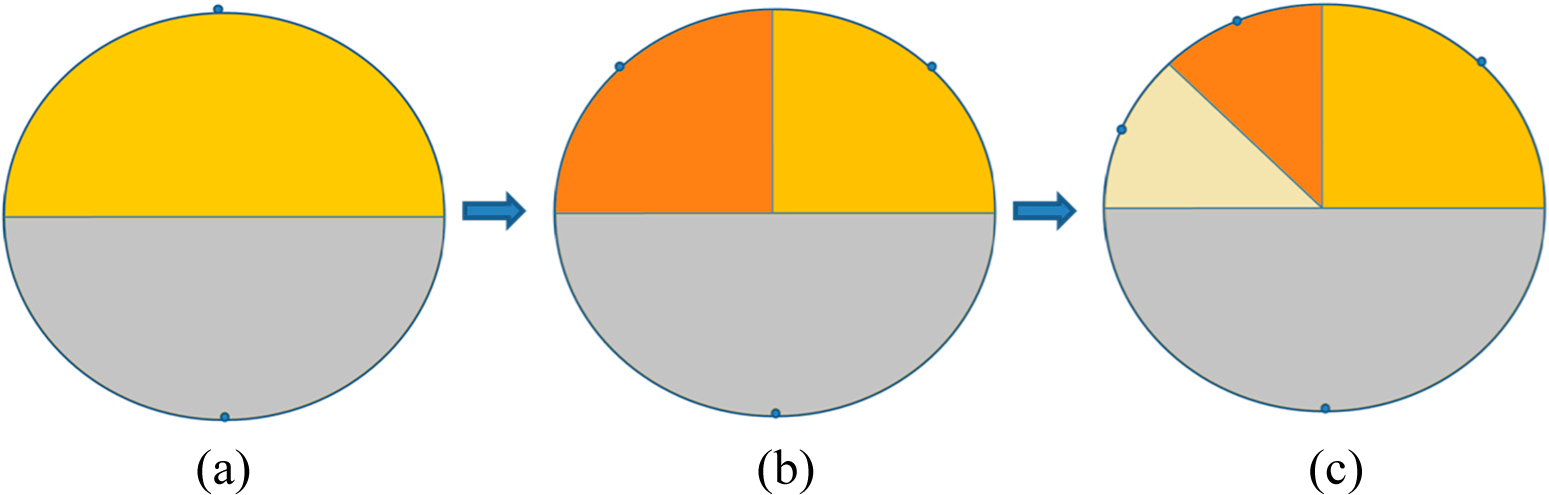
As examples, a two-stage process of two neurons splitting to three neurons and then to four neurons are shown in Figure 5a–c. The corresponding vector A and sita recording the number of splitting times that each neuron went through and the argument of each neuron label point are as follows:

$$\mathbf{A}=[0,0]\to \mathbf{A}=[0,1,1]\to \mathbf{A}=[0,1,2,2]$$

$$\begin{array}{l}\mathbf{sita}=[-\frac{\pi }{2},\frac{\pi }{2}]\to \mathbf{sita}=[-\frac{\pi }{2},\frac{\pi }{2}-\frac{\pi }{2^2},\frac{\pi }{2}+\frac{\pi }{2^2}]=[-\frac{\pi }{2},\frac{\pi }{4},\frac{3\pi }{4}]\\ \to \mathbf{sita}=[-\frac{\pi }{2},\frac{\pi }{2}-\frac{\pi }{2^2},\frac{\pi }{2}+\frac{\pi }{2^2}-\frac{\pi }{2^3},\frac{\pi }{2}+\frac{\pi }{2^2}+\frac{\pi }{2^3}]=[-\frac{\pi }{2},\frac{\pi }{4},\frac{5\pi }{8},\frac{7\pi }{8}]\end{array}$$

• 9. Initialize the new weights of the new generated neurons through circle neighbor strategy (explained in the following “Remarks”) and maintain the weights of nonsplitting neurons. Set the activation number ${\lambda }_i=0$ for the ith neuron, where $i=1,2,\mathrm{...},N+1$, and the iterations $t=1$.
• 10. Perform Steps 3–9 to all $N+1$ neurons with weights illustrated in Step 11.

Remarks:

• A. In the competitive module, ${\alpha }_1$ and ${\alpha }_2$ ( ${\alpha }_2<{\alpha }_1$) denote the leaning rate of the winner neuron and the neighboring neurons respectively. Fixed values or varied values monotonically decreasing with iterations are all acceptable. In the experiment of this paper, we choose the fixed values as ${\alpha }_1=0.09$, ${\alpha }_2=0.0045$.
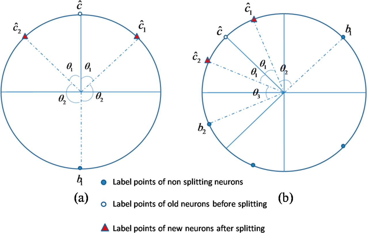
• B. In order to create an ordered topology on the unit disk, the “circle neighbor strategy” is employed to initialize the weights of new neurons. Because the neuron label points are distributed on the unit circle, the circumferential distance between two points is only decided by the angle between corresponding two circle radiuses. For ensuring the close neurons with similar weights, the strategy can be executed as follows.
• ➢ Case 1: the neuron number is 2, i.e., 2 neurons splits to 3 neurons.

As illustrated in Figure 6a, neuron $\widehat{c}$ splits to two neurons ${\widehat{c}}_1$ and ${\widehat{c}}_2$, and the nonsplitting neuron denotes as $b_1$. The angle between radiuses of $\widehat{c}$ and ${\widehat{c}}_1$ (same as that between $\widehat{c}$ and ${\widehat{c}}_2$) is denoted by ${\theta }_1$; The angle between radiuses of $b_1$ and ${\widehat{c}}_1$ (same as that between $b_1$ and ${\widehat{c}}_2$) is denoted by ${\theta }_2$. The initial weights of new neurons can be endowed as follows:

$${\mathbf{W}}_{{\widehat{c}}_1}=\frac{{\theta }_2}{{\theta }_1+{\theta }_2}{\mathbf{W}}_{\widehat{c}}+\frac{{\theta }_1}{{\theta }_1+{\theta }_2}{\mathbf{W}}_{b_1}+\mathbf{R}$$

(14)

$${\mathbf{W}}_{{\widehat{c}}_2}=\frac{{\theta }_2}{{\theta }_1+{\theta }_2}{\mathbf{W}}_{\widehat{c}}+\frac{{\theta }_1}{{\theta }_1+{\theta }_2}{\mathbf{W}}_{b_1}-\mathbf{R}$$

(15)

where R is an random vector satisfying $\left|\right|\mathbf{R}\left|\right|\ll \left|\right|\mathbf{W}\left|\right|$.

• ➢ Case 2: the neuron number $N>2$, i.e., $N$ neurons splits to $N+1$ neurons.

As illustrated in Figure 6b, the angle between radiuses of old neuron $\widehat{c}$ and new neuron ${\widehat{c}}_1$ (same as that between $\widehat{c}$ and ${\widehat{c}}_2$) is denoted by ${\theta }_1$; The angle between radiuses of neighboring neuron $b_1$ and neuron ${\widehat{c}}_1$ is denoted by ${\theta }_2$; The angle between radiuses of neighboring neuron $b_2$ and neuron ${\widehat{c}}_2$ is denoted by ${\theta }_3$. The initial weights of new neurons can be endowed as follows:

$${\mathbf{W}}_{{\widehat{c}}_1}=\frac{{\theta }_2}{{\theta }_1+{\theta }_2}{\mathbf{W}}_{\widehat{c}}+\frac{{\theta }_1}{{\theta }_1+{\theta }_2}{\mathbf{W}}_{b_1}$$

(16)

$${\mathbf{W}}_{{\widehat{c}}_2}=\frac{{\theta }_3}{{\theta }_1+{\theta }_3}{\mathbf{W}}_{\widehat{c}}+\frac{{\theta }_1}{{\theta }_1+{\theta }_3}{\mathbf{W}}_{b_2}$$

(17)

The weight initialization with “circle neighbor strategy” ensures an ordered topology for newly created neurons and old neurons. Besides, all weights of new and nonsplitting neurons could be used in the next competitive learning algorithm which effectively avoids the retraining process.

4. License Plate Character Recognition and Results

In this section, we use the SCDCS-LS based RWNN for license plate character recognition. All character samples are extracted from pictures of Chinese license plates in our experiments. Chinese license plate is composed of seven characters in which the first one is a Chinese character, the second one is an English letter and the remaining ones are numbers or English letters. Two experiments are carried out here. The first one is recognition of English letters on the second position of plate which are the city code of vehicle license. The second one is recognition numbers or English letters on the three to seven positions of plate.

In order to avoid confusion, letters “I” and “O” are not employed in Chinese license plates. And because of the samples of letter “T” are few in number in our sample library, which cannot meet the training and testing requirement, the category of English letters are 23 letters except “I”, “O” and “T” in our experiments.

The character library in our experiments containing character samples extracted from plates which are located from images by algorithms proposed in [1], slant corrected and segmented by algorithms proposed in [5]. Due to the environment factors (for example the weather conditions and light effects etc.) in the process of image acquisition and angle error in slant correction algorithm, some character images which are somewhat distorted are also contained in the library. Several sample examples are shown in Figure 7.

4.1. Example 1: Recognition of English Letters

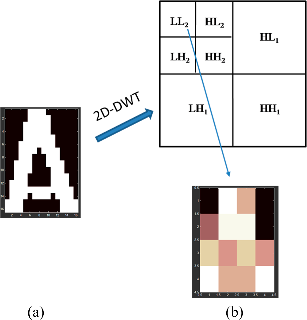
All samples resized as 16×16 pixels are randomly selected from our character library. 40 samples are chosen for training and 20 samples for testing for each type of character (except letters “M”, “N”, “P”, “U”, “V” and “Z” whose testing setshave 19, 16, 13, 12, 11 and 14 samples respectively). The approximation components of 2-level wavelet decomposition (see [25]) are used as features for each character sample (Figure 8), which compose the input vectors of RWNN in our experiment. That is to say, the number of input neurons is 16 in RWNN. The output vectors consist of 23 elements as the ith element being 1 and others being 0 when the samples belonging to the ith letter category.

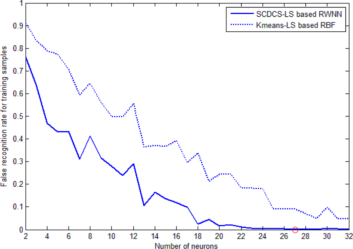
The training patterns’ false recognition rates during learning which correspond to the increasing number of neurons created by the SCDCS-LS algorithm are illustrated by the solid line in Figure 9. In order to testify the effectiveness of the proposed model, the classical RBF network with K-means clustering and LS is used as the classifier to same training patterns. The curve of false recognition rate for K-means-LS based RBF is also drawn as dotted line in Figure 9 for comparison. From Figure 9, it can be seen that the SCDCS-LS based RWNN model has the better performance than the K-means-LS based RBF model. When the number of neurons in the splitting process increases to N = 27 with the corresponding valid neurons number N₁ = 26, the total success recognition rate for training set and testing set of SCDCS-LS based RWNN reaches 99.89% and 99.76% respectively, and after that the false recognition rate will no longer be significantly decrease with newly added neurons. But when the neuron number of K-means-LS based RBF increases to N = 32 as shown in Figure 9, the total success recognition rate for training set and testing set are 95.34% and 96.71% respectively. The detailed recognition results for testing samples by two models are in

Table 1. Recognition results of SCDCS-LS based RWNN for testing samples (Example 1, hidden neuron number N_w = 26).

Structure	16-26-23
Character	A	B	C	D	E	F	G	H	J
Number of testing samples	20	20	20	20	20	20	20	20	20
Number of success recognized samples	20	20	20	20	20	19	20	20	20
Success recognition rate	100%	100%	100%	100%	100%	95%	100%	100%	100%
Character	K	L	M	N	P	Q	R	S	U
Number of testing samples	20	20	19	16	13	20	20	20	12
Number of success recognized samples	20	20	19	16	13	20	20	20	12
Success recognition rate	100%	100%	100%	100%	100%	100%	100%	100%	100%
Character	V	W	X	Y	Z
Number of testing samples	11	20	20	20	14	Total number of testing samples		425
Number of success recognized samples	11	20	20	20	14	Total number of success recognized samples		424
Success recognition rate	100%	100%	100%	100%	100%	Total success recognition rate		99.76%

and

Table 2. Recognition results of Kmean-LS based RBF for testing samples (Example 1, hidden neuron number N_w = 32).

Structure	16-32-23
Character	A	B	C	D	E	F	G	H	J
Number of testing samples	20	20	20	20	20	20	20	20	20
Number of success recognized samples	20	20	20	20	20	20	20	20	20
Success recognition rate	100%	100%	100%	100%	100%	100%	100%	100%	100%
Character	K	L	M	N	P	Q	R	S	U
Number of testing samples	20	20	19	16	13	20	20	20	12
Number of success recognized samples	20	19	19	16	0	20	20	20	12
Success recognition rate	100%	95%	100%	100%	0%	100%	100%	100%	100%
Character	V	W	X	Y	Z
Number of testing samples	11	20	20	20	14	Total number of testing samples		425
Number of success recognized samples	11	20	20	20	14	Total number of success recognized samples		411
Success recognition rate	100%	100%	100%	100%	100%	Total success recognition rate		96.71%

, which adopt 26 and 32 hidden neurons respectively.

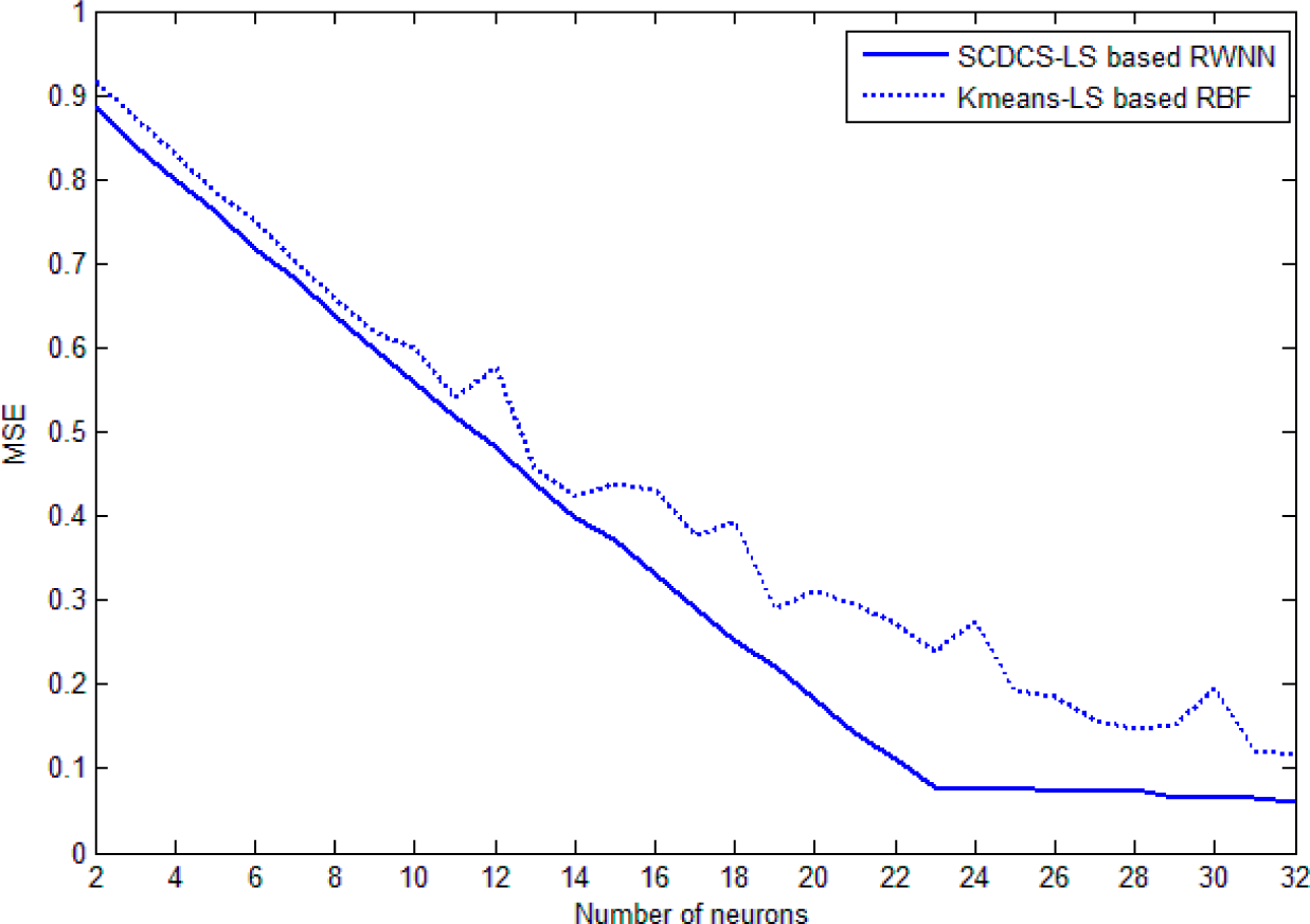
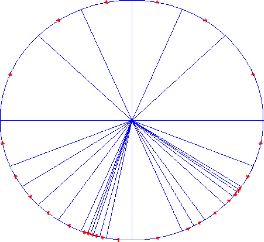
Figure 10 shows the comparative curves of mean square error (MSE) that varying with the increasing number of neurons for SCDCS-LS based RWNN and K-means-LS based RBF. The disk distribution map of 27 neurons got by SCDCS-LS algorithm is drawn in Figure 11.

Table 3. Vectors A and sita of neurons in Figure 11 which record the number of splitting times that each neuron went through and the argument of each neuron label point (neuron number N = 27, valid neuron number N₁ = 26, ★ denotes the invalid neuron).

Neuron label	1	2	3	4	5★	6	7	8	9
A	3	4	4	4	4	6	7	7	6
sita	−2.945	−2.651	−2.454	−2.258	−2.062	−1.939	−1.902	−1.878	−1.841
Neuron label	10	11	12	13	14	15	16	17	18
A	6	4	3	5	5	4	5	6	7
sita	−1.792	−1.669	−1.374	−1.129	−1.031	−0.884	−0.736	−0.663	−0.626
Neuron label	19	20	21	22	23	24	25	26	27
A	7	4	3	2	3	3	3	3	2
sita	−0.601	−0.491	−0.196	0.393	0.982	1.374	1.767	2.160	2.749

illustrates the vector A and sita of these neurons which record the number of splitting times that each neuron went through and the argument of each neuron label point. The comparison results of different models are concluded in

Table 4. Comparision of success recognition rate of different models (Example 1).

Model	Number of hidden neurons	Success recognition rate
		Training	Testing
GD based BP [1,7]	32	94.57%	95.53%
K-means-LS based RBF [27]	32	95.34%	96.71%
SVM [29,30]	–	100%	98.59%
SCDCS-LS based RWNN	26	99.89%	99.76%

. It can be seen that the SVM algorithm can make the highest recognition rate for training samples, but a lower recognition rate for testing samples. The proposed SCDCS-LS based RWNN can get higher recognition rates both for training and testing samples although fewer hidden neurons are employed.

4.2. Example 2: Recognition of Numbers or English Letters

Samples of numbers or English letters are chosen randomly from our character library like experiment 1. Equal numbers of samples in training set and testing set of each character category are employed as experiment 1 too. 16 input features for each sample consists of the approximation components of 2-level wavelet decomposition. 33 output neurons are needed for RWNN here for the 33 character categories corresponding to 23 English letters and 10 numbers.

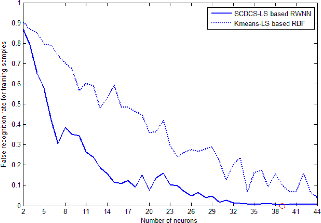
In the experiment of recognition of numbers or English letters samples by SCDCS-LS based RWNN, when the number of neurons in the splitting process increases to $N=39$ with the corresponding valid neurons number $N_1=38$, the total success recognition rate for training set reaches 99.54% and will no longer increase significantly during the splitting process as shown in Figure 12 (the false recognition rate curve is drawn corresponding to neurons splitting from 2 to 44). Adopt the RWNN with $N_1=38$ hidden neurons and parameters got by SCDCS-LS, the total success recognition rate for testing set reaches 99.20%. The detailed results are shown in

Table 5. Recognition results of SCDCS-LS based RWNN for testing samples (Example 2, hidden neuron number N_w = 38).

Structure	16-38-33
Character	A	B	C	D	E	F	G	H	J
Number of testing samples	20	20	20	20	20	20	20	20	20
Number of success recognized samples	20	19	20	20	20	19	20	20	20
Success recognition rate	100%	95%	100%	100%	100%	95%	100%	100%	100%
Character	K	L	M	N	P	Q	R	S	U
Number of testing samples	20	20	19	16	13	20	20	20	12
Number of success recognized samples	20	20	19	16	13	19	20	20	12
Success recognition rate	100%	100%	100%	100%	100%	95%	100%	100%	100%
Character	V	W	X	Y	Z	0	1	2	3
Number of testing samples	11	20	20	20	14	20	20	20	20
Number of success recognized samples	11	20	20	20	14	19	20	19	20
Success recognition rate	100%	100%	100%	100%	100%	95%	100%	95%	100%
Character	4	5	6	7	8	9
Number of testing samples	20	20	20	20	20	20	Total number of testing samples		625
Number of success recognized samples	20	20	20	20	20	20	Total number of success recognized samples		620
Success recognition rate	100%	100%	100%	100%	100%	100%	Total success recognition rate		99.20%

. For comparison, the curve of false recognition rate for K-means-LS based RBF is also drawn as dotted line in Figure 12. When the neuron number of K-means-LS based RBF increases to $N=44$, the total success recognition rate for training set and testing set are 96.24% and 95.84% respectively with detailed recognition results for testing set in

Table 6. Recognition results of K-means-LS based RBF for testing samples (Example 2, hidden neuron number N_w = 44).

Structure	16-44-33
Character	A	B	C	D	E	F	G	H	J
Number of testing samples	20	20	20	20	20	20	20	20	20
Number of success recognized samples	20	0	20	20	20	19	20	20	20
Success recognition rate	100%	0%	100%	100%	100%	95%	100%	100%	100%
Character	K	L	M	N	P	Q	R	S	U
Number of testing samples	20	20	19	16	13	20	20	20	12
Number of success recognized samples	20	19	19	16	13	19	20	20	12
Success recognition rate	100%	95%	100%	100%	100%	95%	100%	100%	100%
Character	V	W	X	Y	Z	0	1	2	3
Number of testing samples	11	20	20	20	14	20	20	20	20
Number of success recognized samples	11	20	20	20	14	19	20	20	20
Success recognition rate	100%	100%	100%	100%	100%	95%	100%	100%	100%
Character	4	5	6	7	8	9
Number of testing samples	20	20	20	20	20	20	Total number of testing samples		625
Number of success recognized samples	20	18	20	20	20	20	Total number of success recognized samples		599
Success recognition rate	100%	90%	100%	100%	100%	100%	Total success recognition rate		95.84%

. It can be seen that, the proposed SCDCS-LS based RWNN shows better performance than the K-means-LS based RBF in recognition of numbers or English letters even though fewer hidden neurons are employed.

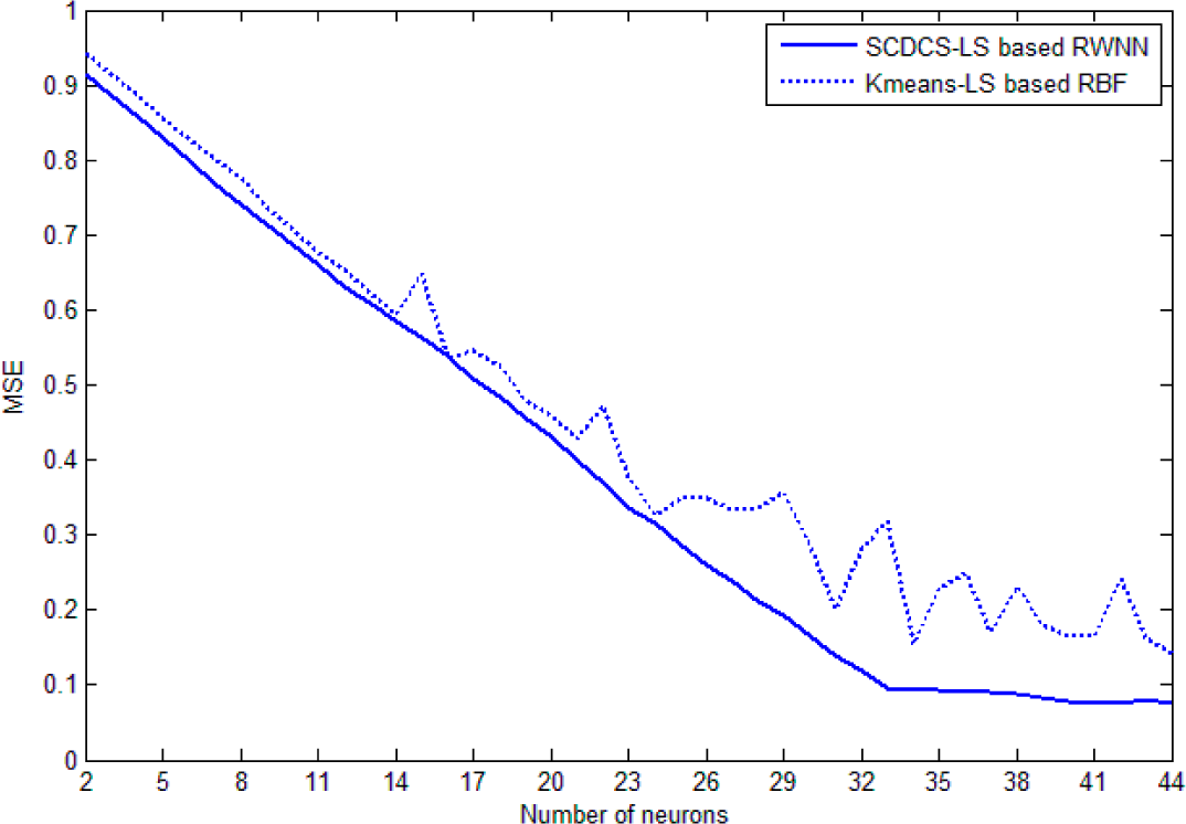
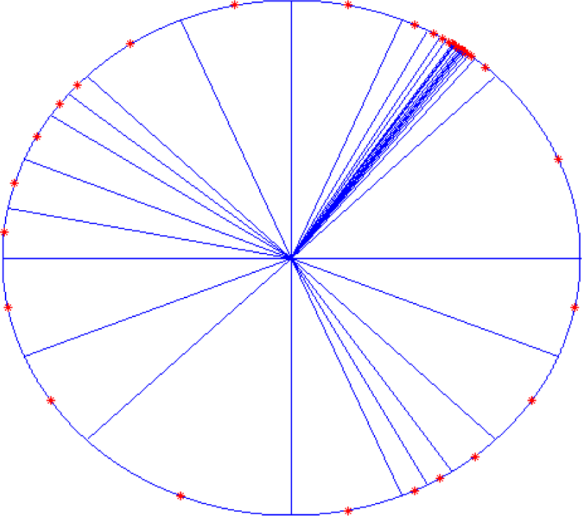
Figure 13 shows the comparative curves of mean square error (MSE) that varying with the increasing number of neurons for SCDCS-LS based RWNN and K-means-LS based RBF for training samples of numbers or English letters. The disk distribution map of 34 neurons got by SCDCS-LS algorithm is drawn in Figure 14.

Table 7. Vectors A and sita of neurons in Figure 14 which record the number of splitting times that each neuron went through and the argument of each neuron label point (neuron number N = 39, valid neuron number N₁ = 38, ★ denotes the invalid neuron ).

Neuron label	1	2	3	4	5	6	7	8★	9
A	3	3	2	3	5	5	4	3	3
sita	−2.945	−2.553	−1.963	−1.374	−1.129	−1.031	−0.884	−0.589	−0.196
Neuron label	10	11	12	13	14	15	16	17	18
A	2	5	7	8	8	9	10	10	8
sita	0.393	0.834	0.896	0.914	0.927	0.936	0.940	0.943	0.951
Neuron label	19	20	21	22	23	24	25	26	27
A	8	9	10	13	13	12	12	13	13
sita	0.963	0.973	0.977	0.979	0.979	0.980	0.981	0.981	0.982
Neuron label	28	29	30	31	32	33	34	35	36
A	7	7	6	5	3	3	3	5	5
sita	0.994	1.019	1.055	1.129	1.374	1.767	2.160	2.405	2.503
Neuron label	37	38	39
A	4	4	4
sita	2.651	2.847	3.043

illustrates the vector $\mathbf{A}$ and $\mathbf{sita}$ of these neurons which record the number of splitting times that each neuron went through and the argument of each neuron label point.

Table 8. Comparision of success recognition rate of different models (Example 2).

Model	Number of hidden neurons	Success recognition rate
		Training	Testing
GD based BP [1,7]	44	90.55%	91.52%
K-means-LS based RBF [27]	44	96.24%	95.84%
SVM [29,30]	–	99.92%	98.56%
SCDCS-LS based RWNN	38	99.54%	99.20%

gives the comparison results of recognition rates using different classifiers. It can be seen that the results are similar to that of example 1. Besides the slightly higher recognition rate for training samples by SVM, the proposed SCDCS-LS based RWNN can get both high recognition rates for training and testing samples.

5. Conclusions

In this paper, a novel learning algorithm of radial wavelet neural network is proposed for license plate character recognition. Based on the competitive learning of SOM, the proposed self-creating disk-cell-splitting algorithm can bore neurons on a disk adaptively according to the distribution of input data and learning goals. The “circle neighbor strategy” employed to initialize weights of new neurons can make an ordered topology on the disk as well as utilize the trained weights which ensures an efficient training process. As a result, a disk map of input data and a RWNN model with proper architecture and parameters could be determined for the recognition task. Experiments of recognition of English letters and recognition of numbers or English letters are implemented for test the effectiveness of our learning algorithm. Compared to the classical RBF network with K-means clustering and LS method, the proposed model can make a better recognition performance even when fewer hidden neurons are employed.