Entropies from Markov Models as Complexity Measures of Embedded Attractors

Abstract

This paper addresses the problem of measuring complexity from embedded attractors as a way to characterize changes in the dynamical behavior of different types of systems with a quasi-periodic behavior by observing their outputs. With the aim of measuring the stability of the trajectories of the attractor along time, this paper proposes three new estimations of entropy that are derived from a Markov model of the embedded attractor. The proposed estimators are compared with traditional nonparametric entropy measures, such as approximate entropy, sample entropy and fuzzy entropy, which only take into account the spatial dimension of the trajectory. The method proposes the use of an unsupervised algorithm to find the principal curve, which is considered as the “profile trajectory”, that will serve to adjust the Markov model. The new entropy measures are evaluated using three synthetic experiments and three datasets of physiological signals. In terms of consistency and discrimination capabilities, the results show that the proposed measures perform better than the other entropy measures used for comparison purposes.

1. Introduction

In the last few years, the complexity analysis of time series has attracted the attention of the research community as a way to characterize different types of signals. The main aim behind this kind of analysis is to capture information about a dynamical system with no a priori knowledge about the behavior of the system nor about the inner relationships among the variables inside it, but only by observing the output during a period of time. In fact, the most important characteristic of the complexity analysis is its ability to capture and quantify non-linear effects present in the underlying system. These effects cannot be characterized using standard methods of signal analysis, which are commonly based on linear assumptions about the dynamics of the system under study [1] (Chapter 1). This kind of analysis has proven to be very useful for characterizing pathophysiological conditions using different biomedical signals [2], for quantifying machinery health conditions [3], Earth science [4] and many other fields of application.

The complexity analysis of time series has its roots in Takens’ embedding theorem that states a way to reconstruct the state space of a system only by using the output of the system during a period of time. Although some information-theoretic-based works make no explicit reference to Takens’ theorem when defining complexity measures, since the early work by Pincus [5], it is clear that the vectors used for the estimation of the correlation sum can be understood as points obtained from a reconstructed state space with the embedding dimension set by default to two and time delay set to one. This idea is also set by Balasis et al. [4], considering that several of the most well-known information-theoretic measures used as complexity measures can also be considered as phase space-based approaches. An important fact of Takens’ theorem is that it demonstrates that under very general conditions, the reconstructed state space contains most of the information of the original state space and also that the mapping between these two spaces is smooth and invertible, i.e., the reconstructed state space is a diffeomorphic version of the original one [6].

Most of the measures applied to characterize reconstructed state spaces are focused on a sub-region of it called the attractor, which can be defined as a set of numerical values toward which a system tends to evolve, for a wide variety of starting conditions of the system [7]. The characterizing measures include fractal dimensions, such as the box counting and correlation dimension (CD), the largest Lyapunov exponent (LLE) and entropy measures. Fractal dimensions are considered as a way to characterize the actual number of degrees of freedom of the underlying system, while LLE is a measure of the separation rate of infinitesimally close trajectories of the attractor [8]. In other words, LLE measures the sensitivity to the initial conditions of the underlying system, since one of the main characteristics of nonlinear systems is the possibility that two trajectories in the state space begin very close and diverge through time, which is a consequence of the unpredictability and inherent instability of the solutions in the state space. However, both LLE and CD assume an underlying deterministic system, and this assumption cannot be satisfied in several contexts [5]. Besides, there exist numerical and algorithmic problems associated with the calculation of LLE, casting doubt about the reliability of its use in real situations [9,10].

To overcome these restrictions, several researchers began to use measures based on information theory. These measures can also capture the complexity and unpredictability of the underlying system with no assumptions about the nature of the signal (i.e., deterministic or stochastic). The most common measure used in this context is the approximate entropy (ApEn) [5], which is a measure of complexity that can be used in noisy and medium-sized datasets. It employs a nonparametric estimate of the probability mass function of the embedding attractor using a Parzen-window method with a rectangular kernel. In order to improve the modeling capabilities of ApEn, several modifications have been proposed in the literature. The first one, called sample entropy (SampEn) [11], was developed to obtain a measure less sensitive to the signal length. Another modification of ApEn is presented in [12,13], and it uses a Gaussian kernel function for the Parzen-window estimator instead of the original rectangular function, leading to a more consistent measure that is less sensitive to small changes in the signal under study (these measures will be explained in more detail in Section 3). Although ApEn-based measures have been applied successfully in several problems [2,11], it is important to highlight that all of these measures are evaluated with no account of the intrinsic time evolution of the trajectories: they only look for quantifying the entropy in terms of the spatial unpredictability of the points forming the trajectories in the attractor, but not taking into account the directions of divergence along time. Let us consider two temporally consecutive points in an attractor; if these two points are close enough, any ApEn-based measure will count them as neighbors. Nevertheless, if they are more distant than an arbitrary threshold, they will not be considered as neighbors no matter if both points remain on the trajectory or if one is far from it (diverging from the trajectory). Such divergence could happen due to, for instance, a bifurcation or simply by a sudden irregularity of the system. In this sense, note that a diverging point could be located either outside of the trajectory or inside it, but a little further away from the threshold defining the neighborhood. In view of this, a more appropriate measure should not treat such points in the same way, since actually, they are different. Nevertheless, in order to discriminate in a better way different kinds of “diverging points”, it should require that the entropy estimator would take into consideration the information about the “main” (or average) trajectory of the system and also should consider the intrinsic dynamical information of the points forming the attractor.

One important aspect that must be considered at this point is the fact that the interest of the complexity analysis of the time series is usually to provide a method able to differentiate among different states or conditions of a system, e.g., healthy vs. pathological; in other words, to provide a relative measure that could be used for comparison purposes, rather than an absolute measure of complexity. Thus, the main aim of the use of a “main trajectory” is to capture the “regular behavior” that a particular system should have in a normal situation, i.e., the expected quasi-periodic deterministic component, and from it, to quantify the irregularities coming out from other components of the system or by irregular changes in the system. Taking into account that some time series include multiple frequency components and also that those systems could be a combination of deterministic and stochastic parts, this paper proposes a way to characterize the entropy of reconstructed attractors assuming that the dynamical dependence of the state variables in the attractor can be modeled as a hidden Markov process. The probability density estimation is carried out using a discrete hidden Markov model (DHMM) [14], whose codebook was adjusted as the principal curve (PC) of the attractor obtained by means of an unsupervised method based on the subspace-constrained mean shift (SCMS) [15]. As originally defined by [16], PC is an infinitely differentiable finite length curve that passes through the middle of the data. Thus, PC can be considered the “profile trajectory”, allowing a better quantification of the unpredictability of the diverging points. From the DHMM, three different entropy measures are obtained: a standard Markov chain entropy [17] (Chapter 4), a conditional state Markov entropy and a recurrence state Markov entropy. With the aim of evaluating their robustness and reliability to different conditions, such as noise and signal length, the proposed measures are analyzed using three synthetic experiments; and in order to test their usefulness in real-life situations, they are also evaluated using three datasets of physiological signals.

The rest of the paper is organized as follows: Section 2 presents the basic concepts of the embedding procedure; Section 3 exposes the principal approach in the state-of-the0art for measuring the complexity of embedded attractors from entropy measures. Next, Section 4 presents the complexity measures based on a Markovian modeling of the embedded attractors. Section 5 shows a series of experiments and results using the proposed measures and compares their performances with other measures found in the state-of-the-art; and finally, Section 6 presents the conclusions.

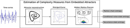
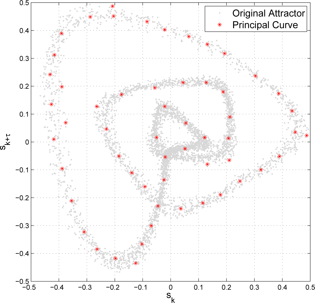
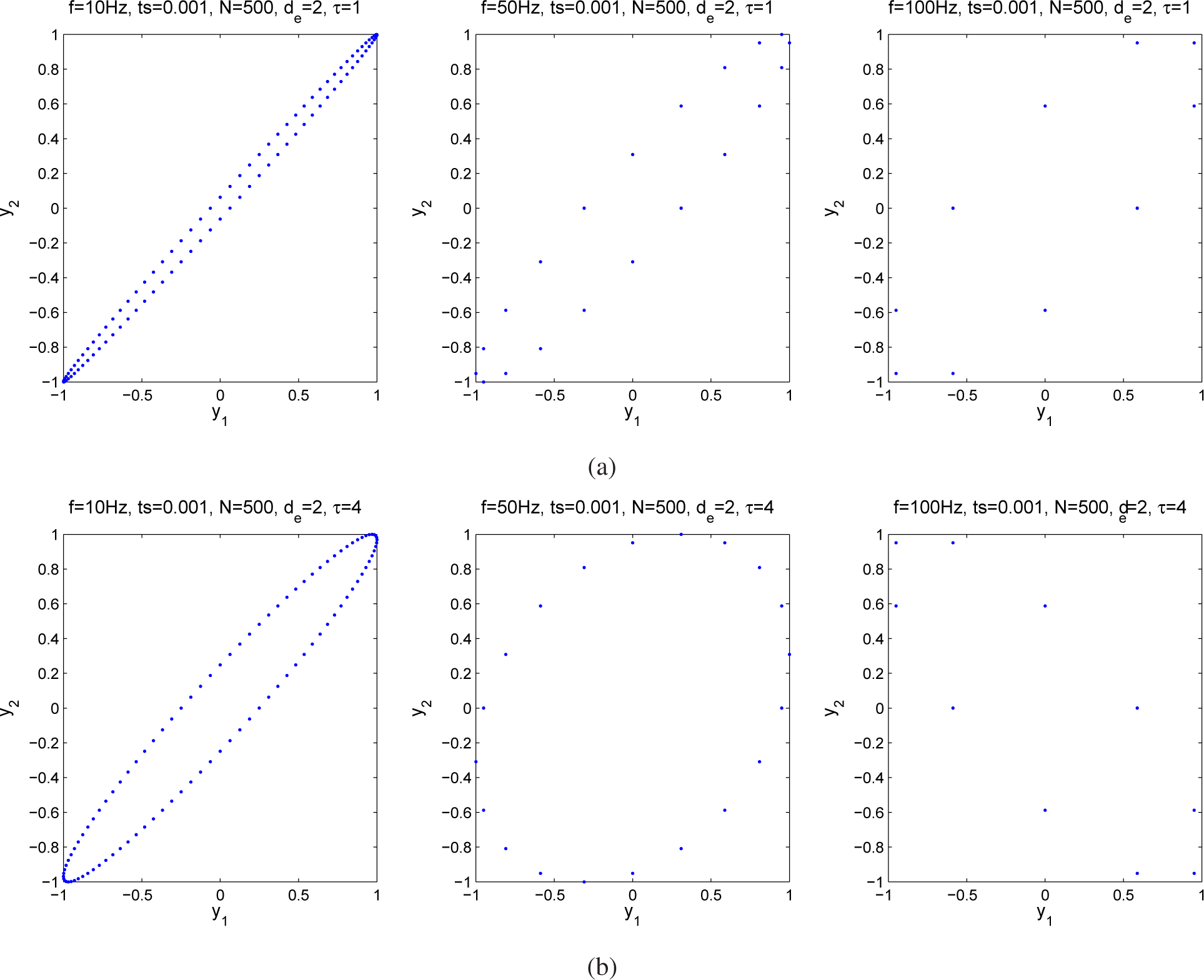
2. Attractor Reconstruction

The most commonly-used technique for state space reconstruction is based on the time-delay embedding theorem [18], which can be written as follows [19]:

Theorem 1 (Time-delay embedding theorem). Given a dynamic system with a d-dimensional solution space and an evolving solution f (x (k)), let s_k be some observation h (x(k)) taken at instant k. Let us also define the lag vector (with dimension d_e and common time lag τ):

$${\mathbf{y}}_k\equiv \left(s_k,s_{k-\tau },s_{k-2\tau },\dots ,s_{k-(d_e-1)\tau }\right)$$

(1)

Then, under very general conditions, the space of vectors y_k generated by the dynamics contains all of the information of the space of solution vectors x(k). The mapping between them is smooth and invertible. This property is referred to as diffeomorphism, and this kind of mapping is referred to as an embedding. Thus, the study of the time series y_k is also the study of the solutions of the underlying dynamical system f (x (k)) via a particular coordinate system given by the observation s_k.

The embedding theorem establishes that, when there is only a single sampled quantity from a dynamical system, it is possible to reconstruct a state space that is equivalent to the original (but unknown) state space composed of all of the dynamical variables [1] (Chapter 3, Section 3.2). The new space is related to the original phase space by smooth and differentiable transformations. The smoothness is essential to demonstrate that all invariant measures of the motion estimated in the reconstructed time delay space are the same as if they were evaluated in the original space, i.e., the geometrical structure of the orbits in the reconstructed state space holds the qualitative behavior of the real state space, allowing the possibility to learn about the system at the source of the observations [6].

3. Entropy Measures

In the field of nonlinear dynamics, the complexity measures are often used to quantify statistically the evolution of the trajectory in the embedded phase space. However, if a time series is considered as the output of a dynamical system in a specific time period, it is regarded as a source of information about the underlying dynamics; therefore, the amount of information about the state of the system that can be obtained from the time series can also be considered a way of complexity.

The fundamental concept to measure the “amount of information” comes from the information theory. Such a concept is termed entropy, which is a measure of the uncertainty of a random variable [17] (Chapter 2). It is a measure of the average amount of information required to describe a random variable. Formally, let X be a discrete random variable with alphabet $\mathcal{X}$ and probability mass function $p(x)=P(X=x),x\in \mathcal{X}$. The Shannon entropy H(X) of a discrete random variable X is defined by:

$$H(X)=-{\displaystyle \sum _{x\in \mathcal{X}}p(x)\log p(x)}$$

(2)

assuming the convention that 0 log(0) = 0 (which is justified by continuity, since x log x → 0 as x → 0), the entropy has the property H ≥ 0. H can also be interpreted as the expected value of the random variable $\log \frac{1}{p(x)}$, where X is drawn according to the probability mass function p(x).

The definition of entropy can be extended to a pair of random variables X and Y with probability mass functions p(x) and p(y), respectively, to provide two additional definitions: the joint entropy given by:

$$H(X,Y)=-{\displaystyle \sum _{x\in \mathcal{X}}{\displaystyle \sum _{y\in \mathrm{Y}}p(x,y)\log p(x,y)}}$$

(3)

where p(x, y) is the join distribution of the X and Y variables; and the conditional entropy, which is the expected value of the entropies of the conditional distributions averaged over the conditioning random variable. It can be expressed as:

$$\begin{array}{l}H(Y|X)=-{\displaystyle \sum _{x\in \mathcal{X}}p(x)}{\displaystyle \sum _{y\in \mathrm{Y}}p(y|x)\log p(y|x)}\\ =-{\displaystyle \sum _{x\in \mathcal{X}}{\displaystyle \sum _{y\in \mathrm{Y}}p(x,y)\log p(y|x)}}\end{array}$$

(4)

The relationship between the definition of both entropies is given by [17] (Chapter 2):

$$H(X,Y)=H(X)+H(Y|X)$$

(5)

The conditional entropy H(Y|X) can be phrased as the uncertainty of the two joint random variables diminished by the knowledge of one of them.

If instead of a random variable, we have a sequence of n random variables X = {X_i}, i = 1, 2, …, n (i.e., a stochastic process), the process can be characterized by a joint probability mass function P (X₁ = x₁, …, X_n = x_n) = p(x₁, x₂, …, x_n). Under the assumption of the existence of the limit, the rate at which the joint entropy grows with n is defined by [17] (Chapter 4):

$$H(\mathit{X})=\underset{n\to \infty }{\lim }\frac{1}{n}H(X_1,X_2,\dots ,X_n)=\underset{n\to \infty }{\lim }\frac{1}{n}{H}_n$$

(6)

Additionally, if the set of random variables are independent, but not identically distributed, the entropy rate is given by:

$$H(\mathit{X})=\underset{n\to \infty }{\lim }\frac{1}{n}{\displaystyle \sum _{i=1}^{n}H(X_i)}$$

(7)

The former mathematical formulation defines the key elements for measuring the amount of information contained in a time series. However, from a practical point of view, there are some assumptions that cannot be satisfied in a real problem. First of all, the time series is always finite; therefore, the condition imposed in Equation (7) will never be met. Moreover, it must be considered that the state of the system is measured at some instants, not in continuous time, and also that the observations can only take a finite number of values; in other words, the time series to be analyzed is a discretized version of the continuous dynamical systems’ output; thus, the entropy measure has to be approximated using different means. In this sense, the most well-known entropy measure that takes into consideration these elements is the Kolmogorov–Sinai entropy (H_KS). In order to approximate it, let the state space be partitioned into hypercubes of content ε^d and the state of the system measured at intervals of time δ. Moreover, let p(q₁, …, q_n) denote the joint probability that the state of the system is in the hypercube q₁ at t = δ, q₂ at t = 2δ, and so on. The H_KS is defined as [20]:

$$H_{KS}=-\underset{\underset{\underset{\epsilon \to 0}{n\to \infty }}{\delta \to 0}}{\lim }\frac{1}{n\delta }{\displaystyle \sum _{q_1,\dots ,q_n}p(q_1,\dots ,q_n)\log p(q_1,\dots ,q_n)}$$

(8)

measuring the mean rate of creation of information. For stationary processes, it can be shown that [20]:

$$H_{KS}=\underset{\delta \to 0}{\lim }\underset{\epsilon \to 0}{\lim }\underset{n\to \infty }{\lim }(H_{n+1}-H_n)$$

(9)

With regard to embedded attractors, H_KS estimates the generation of information by computing the probabilities of nearby points that remain close to the signal trajectory after some time. Numerically, only entropies of finite order n can be computed.

From a practical point of view, the approximate entropy (ApEn)is a practical method proposed as an attempt to estimate H_KS. ApEn is a measure of the average conditional information generated by diverging points of the trajectory [5,21]. Given a signal $s=\left\{s_1,s_2,\dots ,s_{n_s}\right\}$, where s_k is an observation as those defined in Section 2 and n_s is the length of the signal, ApEn can be defined as a function of the correlation sum given by:

$$C_k^{d_e}(r)=\frac{1}{n_s-d_e\tau }{\displaystyle \sum _{j=1}^{n_s-d_e\tau }\mathrm{\Theta }(r-\Vert {\mathbf{y}}_k-{\mathbf{y}}_j)\Vert )}$$

(10)

where Θ is the Heaviside function, which is zero for a negative argument and one otherwise, r is the threshold defining the maximum allowed distance between the points y_k and y_j and the norm $\Vert \cdot \Vert$ is defined in any consistent metric space. For a fixed d_e and r, ApEn is given by:

$$ApEn(d_e,r)=\underset{n_s\to \infty }{\lim }\left[{\mathrm{\Phi }}^{d_e+1}(r)-{\mathrm{\Phi }}^{d_e}(r)\right]$$

(11)

where:

$${\mathrm{\Phi }}^{d_e}(r)=\frac{1}{n_s-(d_e-1)\tau }{\displaystyle \sum _{i=1}^{n_s-(d_e-1)\tau }\ln C_i^{d_e}(r)}$$

(12)

Thus, ApEn is approximately equal to the negative average natural logarithm of the conditional probability that two sequences that are similar for d_e points remain similar, with a tolerance r at the next point. Therefore, a low value of ApEn reflects a high degree of regularity.

The first modification of ApEn presented in [11], called sample entropy (SampEn), was developed to obtain a more independent measure of the signal length than ApEn. SampEn is given by:

$$SampEn(d_e,r)=\underset{n_s\to \infty }{\lim }-\ln \frac{{\mathrm{\Gamma }}^{d_e+1}(r)}{{\mathrm{\Gamma }}^{d_e}(r)}$$

(13)

The difference between Γ and Φ is that the first one does not compare the embedding vectors with themselves (excludes self-matches). The advantage is that the estimator is unbiased [20]. Other modifications of ApEn are based on the change of the Heaviside function in (10) for a smother function (such as a Gaussian kernel) in order to improve the relative consistency of the measure, suppress the discontinuity of the auxiliary function over the correlation sum and to provide less dependence on the threshold parameter r. In this context, two very similar measures have been proposed, the Gaussian kernel approximate entropy (GApEn) [13] and fuzzy entropy (FuzzyEn) [12]. In both cases, the Heaviside function is replaced by:

$$d({\mathbf{y}}_i,{\mathbf{y}}_j)=\exp \left(-{\left(\frac{\Vert {\mathbf{y}}_i-{\mathbf{y}}_j\Vert L}{\gamma }\right)}^h\right)$$

(14)

For GApEn, L = 1, γ = 10 and h = 2, while for FuzzyEn, L = ∞, γ = 1 and h is also set to two.

All of these ApEn-based measures look to quantify the unpredictability of the trajectories in the attractor. From a pattern recognition point of view, the complexity measures, such as ApEn and its derived entropies, use a non-parametric estimation of the probability mass function of the embedding attractor using a Parzen-window method with a Gaussian or a rectangular kernel [22]. However, they only attempt to quantify the divergence of the trajectories of the attractor, but do not take into account that a point, considered as a diverging one, could be: (1) a point that follows the same “regular” trajectory, but falls away from the defined neighborhood region of the previous point due to, for instance, multiple frequency components present in the signal; or, (2) a point completely outside of the trajectory. This is an important difference that cannot be detected and quantified by the measures described so far.

4. HMM-Based Entropy Measures

A Markov chain (MC) is a random process that can take a finite number of m values at certain moments of time (t₀ < t₁ < t₂ < ⋯). The values of the stochastic process change with known probabilities, called transition probabilities. The particularity of this stochastic process is that the probability of change to another state depends only on the current state of the process; this is known as the Markov condition. If such probabilities do not change with time and the steady-state distribution is also constant, the MC is stationary; additionally, if every state of MC can be reached from any other stage (which is called irreducible) and all of the states are aperiodic and non-null recurrent, the MC is considered ergodic [23]. Let $\mathit{X}=\left\{X_{t_i}\right\}$ be a stationary MC, where $X_{t_i}$ is the state at the time t_i, which takes values in the finite alphabet $\mathcal{X}$. The MC is completely determined by the set { π, K} where:

• π = {π_i}, i = 1, 2, …, m is the stationary distribution, where m is the number of states in the MC and π_i = P(X_t = i) as t → ∞ being the probability of ending at the i-th state independent of the initial state.
• K = {K_ij}, 1 ≤ i, j ≤ m is the transition kernel of the MC, where K_ij = P(X_t+1 = j|X_t = i) is the probability of reaching the j-th state at time t + 1, coming from the i-th state at time t.

From this definition, the entropy rate of a MC is given by [17] (Chapter 4):

$$H(\mathit{X})=-{\displaystyle \sum _{ij}{\pi }_i{K}_{ij}\log K_{ij}}$$

(15)

The assumption that the time series under analysis would satisfy the ergodic conditions of the model comes from the fact that the proposed approach tries to model the intrinsic dynamic of reconstructed attractors, which are extracted from processes with some kind of quasi-periodic behavior. Moreover, in many cases there are multi-frequency components involved in the process, as well as nonlinear phenomena, such as bifurcations and stochastic components, inducing variability to the state of the system. The presence of different kinds of “diverging points” present in the attractor ((i) those due to multi-frequency components; and (ii) those due to nonlinear phenomena, such as bifurcations or sudden changes in the dynamic of the system) requires that the model could reach any state from any other or remain in one state multiple times. The first of the pointed out requirements matches with the assumption of an irreducible MC. Additionally, according to [23], a sufficient condition to ensure that a state is aperiodic is if it has a self-loop, which satisfies the second requirement. On the other hand, taking into account the quasi-periodicity of the pointed processes and also that the MC is finite, the states can be assumed to be non-null recurrent. Bearing all of this in mind, we believe that the assumption of ergodicity is reasonable.

Analyzing Equation (15), it is possible to observe that the entropy measure is a sum of the individual Shannon entropy measures for the transition probability distributions of each state, weighted with respect to the stationary probability of its corresponding state.

According to [24], due to the fact that at a time t, the current state of a dynamical system provides all of the information necessary to calculate future states, the sequence of states of a dynamical system satisfies the Markov condition. Nonetheless, considering that in several real-time series there is a combination of both deterministic and stochastic components, it cannot be completely modeled by means of a Markov chain. There exist some processes that can be seen like a Markov chain, whose outputs are random variables generated from probability functions associated with each state. Such processes are called hidden Markov processes (HMP) [25]. An HMP can also be understood as a Markov process with noisy observations, providing a nonlinear stochastic approach that is more appropriate for signals with noisy components [26].

Formally, let Z = {Z_t} denote a noisy version of X = {X_t} corrupted by discrete memoryless perturbations, which takes values in the finite alphabet $\mathcal{Z}$. C will denote the channel transition matrix, i.e., the $|\mathcal{X}|\times |\mathcal{Z}|$ matrix with entries C(x, z) = P(Z_t = z|X_t = x). Z is then the HMP; since the states of the Markov process cannot be identified from its output (the states are “hidden”). The distribution and entropy rate H(Z) of an HMP are completely determined by the pair {K, C}; however, the explicit form of H(Z) as a function of such a pair is unknown [25]. On the other hand, let us consider the joint entropy H(X, Z), which, according to Equation (5), can be expressed as:

$$H(\mathit{X},\mathit{Z})=H(\mathit{X})+H(\mathit{Z}|\mathit{X})$$

(16)

where H(X) is the entropy of the Markov process (Equation (15)) and H(Z|X) is the conditional entropy of the stochastic process Z given the Markov process X. Therefore, in the same way as in Equation (15) and taking into account that the noise distributions in each state of the Markov process are conditionally independent of each other, it is possible to establish an entropy measure of the HMP as the entropy of the Markov process plus the entropy generated by the noise in each state of the process. The conditional entropy rate of Z given X can be expressed as [27]:

$$H(\mathit{Z}|\mathit{X})=\underset{n\to \infty }{\lim }H(Z_n|X_n)=E\left\{H\left(Z_n|X_n\right)|X_n\right\}$$

(17)

The advantage of using the entropy estimations in Equations (15) and (17) or their combination, instead of the ApEn-based measures mentioned before, is that the imposed MC characterizes the divergence of the trajectories and the directions into the state space in terms of the transitions between regions provided by the MC states, whilst the HMP quantifies the instability of the trajectories in terms of the noise level or scatter in every state of the process [10,24].

In addition to the mentioned entropies, another interesting measure that can be estimated from the Markov model is the recurrence-state entropy (RSE), which can be seen as a regularity measure of the trajectories visiting the states defined by the MC. In other words, the variability in the number of steps employed for a trajectory to perform a whole loop in the MC (leaving from one particular state and reaching it again) can reflect the stability of the trajectories along time, i.e., frequency perturbations present in the signal. In the following, the practical aspects of the implementation of the measures described in this section will be presented.

4.1. Estimation of the HMM-Based Entropies

The whole Markov model described before is known as a hidden Markov model with a finite observation alphabet (discrete hidden Markov model (DHMM)) [28]. A DHMM is characterized by the set {π, K, B}, where π and K remain as described before (Section 4), and B is defined as follows [28]:

• B = {B_ij}, i = 1, 2, …, m, j = 1, 2, …, b is the probability distribution of the observation symbols, being B_ij = P(Z_t = υ_j|X_t = i), where Z_t is the output at time t, υ_j are different symbols that can be associated with the output and b is the total number of symbols.

All parameters are subject to standard stochastic constraints [28].

Training a DHMM requires a previous definition of the set Ψ = {υ_j}, which has typically been found by means of unsupervised clustering methods, such as linear vector quantization or k-means [30], that require a prior setting of the number of clusters. However, for attractor modeling, the estimation of the PC of the attractor is more interesting, since it can be considered as the “profile” trajectory, and its points can be used to construct Ψ. There are different methods to estimate PCs, in this work, the subspace-constrained mean shift (SCMS) method proposed in [15] was employed, because it provides very stable estimations and good convergence properties [31]. The SCMS is based on the well-known mean shift (MS) algorithm [32], which is a procedure to find the nearest stationary point of the underlying density function and is able to detect the modes of the density. SCMS is a generalization of MS that iteratively tries to find modes of a pdf in a local subspace. It can be used with parametric or non-parametric pdf estimators that are, at least, twice continuously differentiable. Formally, let f be a pdf on R^D; the d-dimensional principal surface is the collection of all points x ∈ R^D where the gradient ∇f(x) is orthogonal to exactly D − d eigenvectors of the Hessian of f, and the eigenvalues corresponding to these eigenvectors are negative [31]. For the PC (which is the interest of this paper), the one-dimensional principal surface is the collection of all points x ∈ R^D at which the gradient of the pdf is an eigenvector of the Hessian of the pdf, and the remaining eigenvectors of the Hessian have negative eigenvalues; i.e., a principal curve is a ridge of the pdf, and every point on the principal curve is a local maximum of the pdf in the affine subspace orthogonal to the curve [31]. SCMS uses a simple modified MS algorithm to iteratively find the set of points according to the previous PC definition [15]. Figure 1 depicts a reconstructed attractor obtained from 200 ms of a normal speech recording and its principal curve obtained with the SCMS algorithm.

On the other hand, each point in the PC is considered as the centroid of one state of the MC (the number of points in the PC corresponds to n_θ); therefore, it is very easy to estimate the kernel transition matrix K, only by counting the transitions between states and converting them into probabilities. Moreover, taking into account the quasi-periodicity of the pointed processes, some kind of oscillatory behavior could be expected for the Markov chains estimated from the reconstructed attractors. Thus, the final state of the process depends on the length of the recorded time series, and it will not tend to some states notoriously more than others. Therefore, the stationary distributions π can be assumed as uniform. From Equation (15), the Markov chain entropy H_MC can be defined as:

$$H_{MC}=-\frac{1}{m}{\displaystyle \sum _{ij}{K}_{ij}\log K_{ij}}$$

(18)

From the MC, it is also possible to associate every point in the attractor with one of the states in order to get an estimation of the conditional HMP entropy (H_HMP) in (17) and, of course, of the joint probability in (16). In this work, the conditional H_HMP for each state i was estimated using two different non-parametric entropy estimators (Shannon and Renyi’s entropies, respectively) given by [33]:

$${\widehat{H}}_R^i=\frac{1}{1-\alpha }\log \left[\frac{1}{n_w^{\alpha }}{\displaystyle \sum _{j=1}^{n_w}{\left({\displaystyle \sum _{i=1}^{n_w}{\kappa }_{\sigma }(v_i-v_j)}\right)}^{\alpha -1}}\right]$$

(19)

and:

$${\widehat{H}}_S^i=-\frac{1}{n_w}{\displaystyle \sum _{j=1}^{n_w}\log \left(\frac{1}{n_w}{\displaystyle \sum _{i=1}^{n_w}{\kappa }_{\sigma }(v_i-v_j)}\right)}$$

(20)

where n_w is the number of points associated with the current MC state and σ is the window size of the kernel function κ (similar to r in the ApEn-based entropies). The order of Renyi’s entropy estimator α in all cases was set to two. Since the probability density functions of every state are independent of each other, the whole H_HMP can be defined using the Shannon and Renyi estimators respectively as:

$$H_{HM{P}_S}=\frac{1}{m}{\displaystyle \sum _{i=1}^m{\widehat{H}}_S^i;}{H}_{HM{P}_R}=\frac{1}{m}{\displaystyle \sum _{i=1}^m{\widehat{H}}_R^i}$$

(21)

which, according to Equation (17), corresponds to the result of averaging H(Z|X_t = x) over all possible values x that X_t may take.

Finally, for the estimation of RSE, the number of steps among consecutive visits to the same state are calculated (avoiding temporal correlations), and conventional Shannon and Renyi’s estimators [34] were employed to measure the variability of such numbers. The whole H_RSE was estimated as the mean of the recurrence-state entropies over all of the MC states. Formally, let η_i(j) be the number of times that a whole loop around the state i took j steps; the Shannon and Renyi estimators of H_RSE can be respectively defined as:

$$H_{RS{E}_S}=-\frac{1}{m}{\displaystyle \sum _{i=1}^m{\displaystyle \sum _{\forall j}\frac{{\eta }_i(j)}{{\displaystyle {\sum }_k{\eta }_i(k)}}\log \left(\frac{{\eta }_i(j)}{{\displaystyle {\sum }_k{\eta }_i(k)}}\right)}}$$

(22)

$$H_{RS{E}_R}=\frac{1}{m}{\displaystyle \sum _{i=1}^m\left[\frac{1}{1-\alpha }\log \left({\displaystyle \sum _{\forall j}{\left(\frac{{\eta }_i(j)}{{\displaystyle {\sum }_k{\eta }_i(k)}}\right)}^{\alpha }}\right)\right]}$$

(23)

5. Experiments and Results

In order to evaluate the performance of the proposed measures, some synthetic tests taken from [12] were applied to the proposed measures. Mainly, the tests try to evaluate the dependence of the measures on the signal length and on the parameter r, as well as the sensitivity to noise. It is important to note that regarding the three entropy measures introduced in this work, only H_HMP depends on the threshold r.

In addition to the synthetic tests, the measures developed were used in four experiments to characterize three different datasets of physiological signals. The first dataset is composed of electroencephalographic (EEG) signals from three groups, H (healthy), E (epileptic subjects during a seizure-free interval) and S (epileptic subjects during a seizure). The database contains 500 recordings (200 H, 200 E and 100 S), whose length is 4097 data points with a sampling frequency of 173.61 Hz. The details of the data can be found at [35].

The second dataset was developed by The Massachusetts Eye and Ear Infirmary (MEEI) Voice & Speech Lab [29]. Due to the different sampling rates of the recordings stored in this database, a downsampling with a previous half band filtering was carried out, when needed, in order to adjust every utterance to a 25-kHz sampling rate. Sixteen bits of resolution were used for all of the recordings. The registers contain the sustained phonation of the/ah/vowel from patients with a variety of voice pathologies: organic, neurological and traumatic disorders. A subset of 173 registers of pathological and 53 normal speakers has been taken according to those enumerated in [36].

The third dataset is available at Physionet [37] and contains electrocardiographic (ECG) recordings from patients suffering from apnea. The samples come from polysomnographies recorded at the sleep laboratory of the Philipps Universität in Marburg, Germany. They are ECG continuous recordings containing all of the events that occur during a night, including apneas, arousals, movements and also some wakefulness episodes. The inclusion criteria of the subjects are reported in the Physionet website and in [38]. The ECG recordings were acquired using standard procedures at a sampling frequency of 100 Hz, with 16 bits of resolution. These recordings were subdivided into three groups: apneic patients (Class A, with more than 100 min in apnea), borderline patients (Class B, with total apnea duration more than 5 and less than 99 min) and control or normal patients (Class C, with less than 5 min in apnea). During a preprocessing stage, all of the recordings were split into segments of one minute long and labeled as normal (7347 min) or containing apnea episodes (4246 min). The database also contains the heart rate variability (HRV) sequence derived from the ECG recordings. Experiments were also performed with the HRV sequences.

5.1. Results

According to the experiments, the results are split into two subsections: the first is dedicated to the results obtained using synthetic data; and the second to the tests carried out using real-life physiological signals.

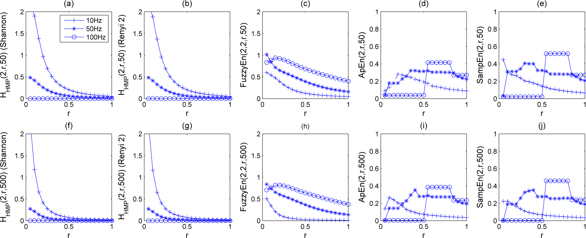
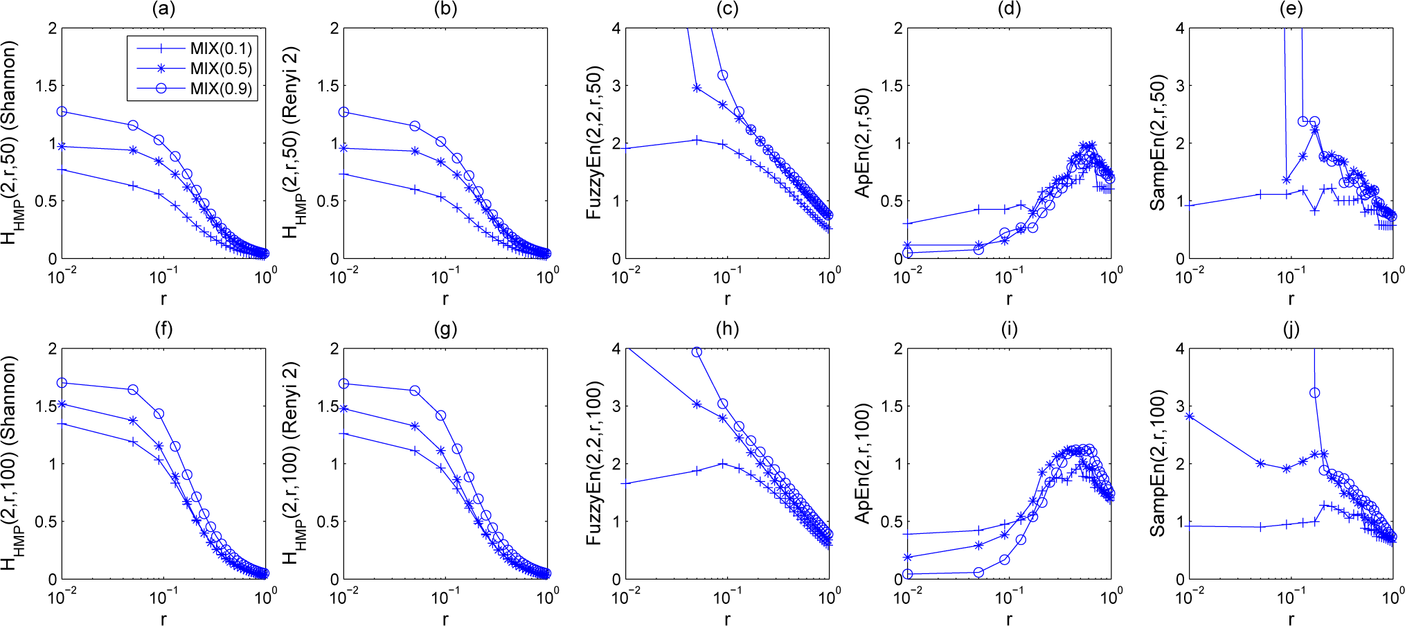
5.1.1. Synthetic Sequences

Figure 2 depicts the values obtained for H_HMP (using Shannon and Renyi’s entropy estimators) along with those obtained with FuzzyEn, ApEn and SampEn for three periodic sinusoids of different frequencies f₁ = 10 Hz, f₂ = 50 Hz and f₃ = 100 Hz, as well as two different signal lengths of N = 50 and 500 points. This experiment has been reproduced as described in [12] assuming a sampling frequency f_s = 1000 Hz, a time delay τ = 1 and an embedding dimension d_e = 2. In view of the results depicted in Figure 2, it is possible to observe that both H_HMP estimations provide very similar results. Furthermore, the values obtained for H_HMP are quite similar for both lengths evaluated, being smaller for bigger N values. Since H_HMP is based on a non-parametric estimation using a Gaussian kernel and in contrast to ApEn-based measures, it shows a smooth behavior and does not change abruptly with respect to small changes in r. The original definition of H_HMP, Equations (19) and (20), used σ instead of r. Although they state for different concepts a window size of the kernel function and neighborhood threshold, respectively, during the experiments with H_HMP, the reader must interpret them as equal. On the other hand, and also in contrast to the ApEn-based measures, H_HMP presents also a good consistency, because there is no crossing among the plots corresponding to different frequencies. These properties are desirable for any entropy estimator.

A more detailed comparison of FuzzyEn with respect to H_HMP in Figure 2 shows that for the first one, the larger the frequency of the sinusoid, the larger the entropy values obtained, whereas for the second one, the larger the frequency, the smaller the entropy. The explanation given to this phenomenon for FuzzyEn in [12] is that high frequency sinusoids appear to be more complex, which is lightly inaccurate, being an undesirable effect of the methods used for estimation; such an empirical result is due to the windowing effect and the need to fix a sampling frequency (f_s) for comparing sinusoids of different fundamental frequencies (f_a) and does not match well with the expected theoretical results, since from an information point of view, it should be zero for any discrete periodic sinusoid of infinite length [39]. This phenomenon is discussed in the Appendix.

Another important point to highlight is that, in most applications (also in [12]), the time delay used for the attractor reconstruction is set to one. Nonetheless, the right choice of the optimum τ improves the characterization of the nonlinear dynamics of time series with long-range linear correlations and an autocorrelation function decaying slowly [40]. The vectors y_k in the correlation sum (Equation (10)) match the vectors defined by Taken’s theorem perfectly, which established that a proper embedding dimension and time delay must be found in order to achieve good results. For many practical purposes, the most important embedding parameter is the product d_eτ of the time delay and the embedding dimension, rather than the embedding dimension and time delay alone [1] (Chapter 3, Section 3.3). The reason is that d_eτ is the time span represented by an embedding vector. However, usually, each of the embedding parameters are estimated separately. The most employed method for the estimation of d_e is the false nearest neighbors method [41] and the first minimum of the auto-mutual information or the first zero crossing of the autocorrelation function for τ. Regarding Figure 3a, it is possible to observe that for f = 10 Hz and τ = 1, the attractor furls around the main diagonal. However, a proper τ estimation (in this case τ = 4) returns the elliptical shape of the embedded attractor, and therefore, a proper selection of the time delay should help to compensate for the effect of the sampling frequency.

For the case of H_HMP, since the entropy is estimated depending on the states of a Markov chain, for f = 10 Hz, each state of the MC will contain several points of the attractor, whilst for f = 100 Hz, the distance among consecutive points increases (Figure 3a), so each state will contain only copies of the same point (from different periods), resulting in an entropy tending to zero as f_a increases. It is worth emphasizing that a proper attractor reconstruction plays an important role in the reliability of the measures that can be estimated from it [1] (Chapter 3).

Unlike H_HMP- and ApEn-based entropies, the other two proposed measures, H_MC and H_RSE, do not depend on the parameter r; therefore, they were only analyzed regarding the frequency, f_a, and signal length, N.

Table 1. Values of entropy measures for perfect sinusoids of different frequencies (f_i) and signal lengths (N). MC, Markov chain; RSE, recurrence-state entropy.

fi	N	HMC		HHMP		HRSE		ApEn	SampEn	FuzzyEn
		S*	R**	S	R	S	R
10	50	1.21	1.07	1.38	1.37	0.75	0.67	0.18	0.28	0.48
	500	1.01	0.76	0.66	0.65	0.96	0.70	0.24	0.19	0.21
50	50	0.30	0.28	0.33	0.33	0.26	0.23	0.18	0.31	0.72
	500	0.12	0.10	0.14	0.14	0.11	0.09	0.14	0.19	0.65
100	50	0.00	0.00	0.00	0.00	0.00	0.00	0.04	0.02	0.94
	500	0.00	0.00	0.00	0.00	0.00	0.00	0.00	0.00	0.82

^*Shannon estimator

^**Renyi estimator

shows the entropy values obtained for the aforementioned synthetic sinusoids. For those entropy measures depending on r, this parameter was a priori set to 0.15. As expected, the Markov-based entropy measures tend to zero, because for perfect sinusoids, there is no unpredictability with respect to the state transition (H_MC) or recurrence (H_RSE); in other words, for an embedded attractor from a perfect sinusoid, the conditional entropy of one point given the previous one (Markov condition) is zero. The length of the signal affects the values obtained for all of the measures, mainly because the more periods, the larger the number of points of the attractor falling in the same positions, implying that the random process becomes more predictable; therefore, its entropy decreases. This is an important property of the proposed measures: they characterize the attractor from a dynamical point of view, instead of in a static way, such as ApEn-based entropies.

The next experiment consists of estimating the complexity of three MIXprocesses [12], defined as:

$$MIX{(\rho )}_j=(1-Z_j)X_j+Z_j{Y}_j$$

(24)

where $X_j=\sqrt{2}$ sin $(2\pi j/12)$ for all j; Y_j are i.i.d. uniform random variables on the interval $\left[-\sqrt{3},\sqrt{3}\right]$; and Z_j are i.i.d. Bernoulli random variables with parameter ρ. The larger ρ is, the more irregular the process becomes. Figure 4 depicts the values of H_HMP, FuzzyEn, ApEn and SampEn statistics measuring the complexity of three different MIX processes. It is possible to observe that H_HMP has a similar consistency to FuzzyEn with respect to the values of complexity given to the processes under analysis, but H_HMP has less dependence on the parameter r, because H_HMP takes values in a narrower interval. Additionally, comparing Figures 4b and 4g against 4c and 4h, the results demonstrate being more consistent for short series. For H_MC and H_RSE,

Table 2. Values of Markovian entropies measuring the complexity of MIX(0.3), MIX(0.5) and MIX(0.7)). For H_HMP, the values were estimated using r = 0.15 × std(signal).

ρ	N	HMC		HHMP		HRSE
		S	R	S	R	S	R
0.3	50	0.64	0.59	0.63	0.61	0.56	0.56
0.3	100	0.96	0.88	0.59	0.56	0.94	0.89
0.5	50	0.93	0.91	0.64	0.62	0.57	0.57
0.5	100	1.31	1.26	0.80	0.78	1.09	1.08
0.7	50	0.83	0.80	0.83	0.82	0.90	0.62
0.7	100	1.22	1.18	0.81	0.79	1.16	1.14

shows the results obtained for the Shannon and Renyi estimators. It is possible to observe that these measures present also a good consistency regarding the complexity of the MIX processes. However, for lower ρ values, there is a stronger dependence on the length of the signal.

The next experiment looks for analyzing the effect of noise in the values provided by the entropy measures. It consists of evaluating the complexity of time series obtained from the Logistic map given by:

$$s_i{}_{+1}=R{s}_i(1-s_i)$$

(25)

for R = {3.5, 3.7, 3.8} and also by adding Gaussian noise components with different noise levels, N = {0, 0.1, 0.2, 0.3}. It is important to note that the logistic map produces periodic dynamics for R = 3.5 and chaotic dynamics for R = {3.7, 3.8}.

Table 3. Entropy values obtained from the logistic system for different R and noise level (NL). The parameter r was set to 0.25.

R	NL	HMC		HHMP		HRSE		ApEn	SampEn	FuzzyEn
		S	R	S	R	S	R
3.5	0.0	0.00	0.00	0.00	0.00	0.00	0.00	0.01	0.00	0.28
	0.1	0.85	0.74	0.23	0.22	1.90	1.67	0.08	0.07	0.48
	0.2	1.40	1.17	0.85	0.83	2.56	2.07	0.61	0.56	0.82
	0.3	1.44	1.28	1.33	1.31	2.23	2.37	0.90	0.88	1.03
3.7	0.0	0.84	0.74	0.43	0.42	3.41	2.68	0.38	0.38	0.77
	0.1	1.10	0.95	0.67	0.66	3.38	2.73	0.49	0.49	0.89
	0.2	1.58	1.43	1.54	1.51	2.83	2.98	0.86	0.81	1.10
	0.3	1.77	1.63	2.65	2.02	2.74	3.11	1.10	1.13	1.29
3.8	0.0	1.10	0.98	0.40	0.39	3.63	3.28	0.47	0.47	0.99
	0.1	1.22	1.03	0.72	0.70	3.75	3.52	0.58	0.59	1.14
	0.2	1.78	1.65	1.53	1.49	3.37	3.25	0.92	0.90	1.31
	0.3	1.83	1.68	2.14	2.10	2.42	2.36	1.19	1.24	1.55

shows the results of this experiment for the six different entropy measures. According to the results, the measures that kept the best consistency in the presence of noise are H_MC, ApEn, SampEn and FuzzyEn; H_HMP and H_RSE showed good consistency for signal-to-noise relationships lower than 0.2.

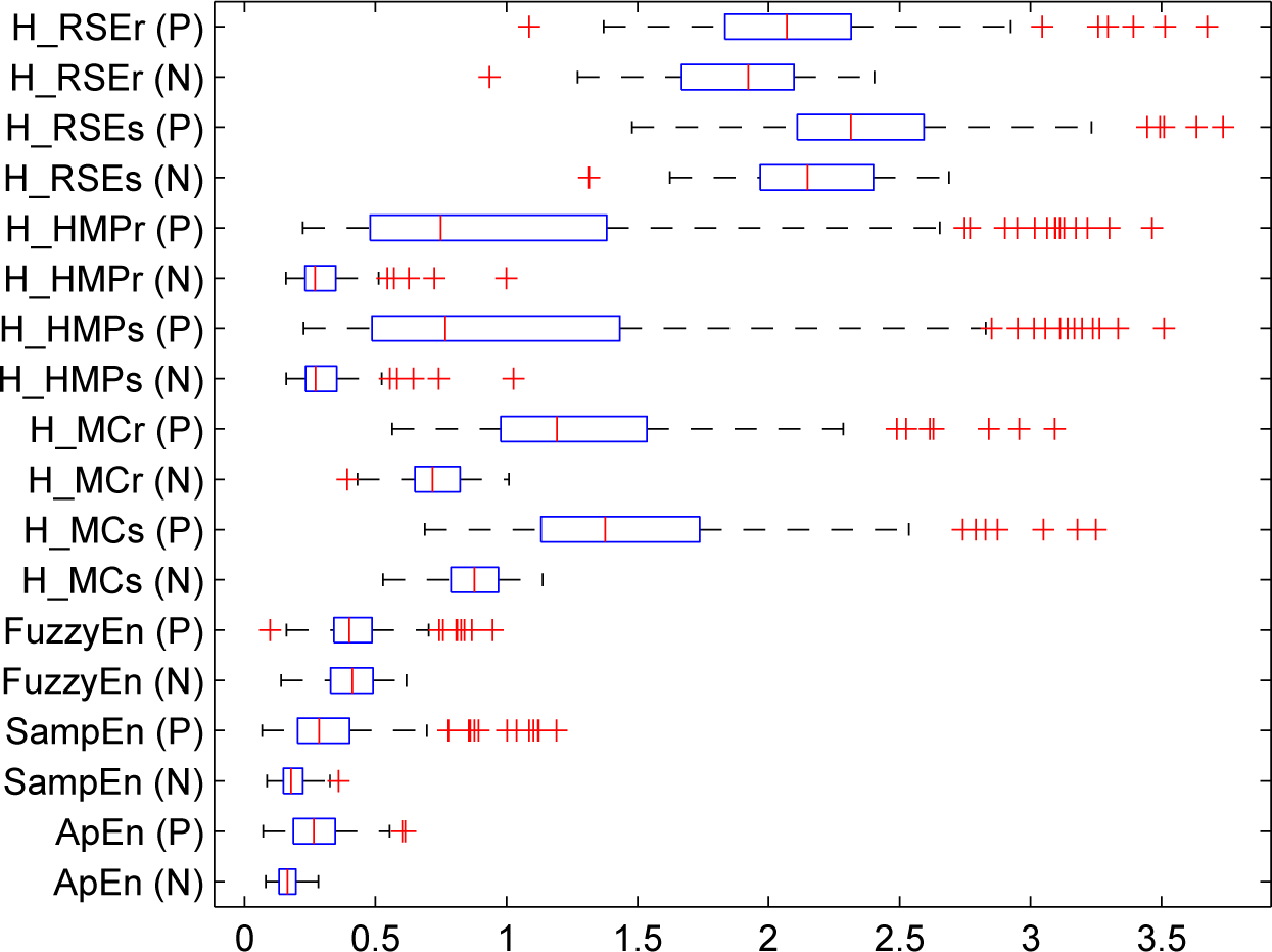
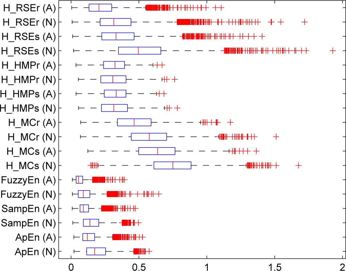
5.1.2. Real-Life Physiological Signals

The following experiments look for demonstrating the usefulness of the Markovian entropy measures in the characterization of real time series. In all of the real situations, the embedding parameters were estimated using the methods described in [1] (Chapter 3) and [41]. The ability of the six entropy measures (including the ApEn-based entropies) to characterize EEG signals from three different classes is shown in Figure 5. SampEn and FuzzyEn performed very well, separating H from E and S, but not so good differentiating E from S, although several values were considered as outliers. In both cases, FuzzyEn performs a little better than SampEn. On the other hand, each of the proposed Markovian entropies performed different for this dataset, since they respectively characterize different aspects of the underlying system. The two estimators of H_HMP performed similar to SampEn; however, H_MC and H_RSE are clearly able to differentiate between S and E groups. This indicates that these measures could be used together to improve the performance of an automatic recognition system, since they provide complementary discriminant information.

In addition to the EEG signals, the entropy measures were also evaluated to characterize voice recordings from pathological and normal speakers. Figure 6 shows the ability of the entropy measures to differentiate both groups. In this case, the parameter r was set to 0.35 × std(signal), as recommended in [10]. Figure 6 shows a similar behavior for ApEn and SampEn, although the pathological group for SampEn is more disperse. On the other hand, H_MC and H_HMP performed very well at separating both classes, whilst H_RSE behaves similarly to SampEn. It is clear from Figure 6 that normal samples can be grouped with less dispersion than the pathological ones. Lastly, the entropy values provided by FuzzyEn let the two groups completely overlap.

In the last experiment, the ability of the entropy measures as indicators of the presence (or absence) of the apnea disorder was evaluated using ECG and HRV sequences. Figure 7 shows the box plots obtained from HRV sequences labeled as normal (N) and apnea (A). None of the entropy measures is able to differentiate the two classes perfectly. However, H_RSE presents the best performance among the measures evaluated. The performance of the measures was also evaluated using the ECG recordings directly; nevertheless, the ApEn-based feature showed a better behavior applied to the HRV sequences, whilst the Markov-based features presented a more stable behavior.

Table 4. Performance of the entropy measures discriminating the different classes in the EEG, voice pathology and apnea (ECG and heart rate variability (HRV)) datasets, according to the Fisher class separability index (FI) and the one-way ANOVA test.

Measures	Datasets
	EEG		Voice		ECG		HRV
	FI	ANOVA	FI	ANOVA	FI	ANOVA	FI	ANOVA
ApEn	0.48	p < 0.001	0.69	p < 0.001	0.64	p < 0.001	0.69	p < 0.001
SampEn	0.48	p < 0.001	0.34	p < 0.001	0.08	v < 0.001	0.83	p < 0.001
FuzzyEn	0.80	p < 0.001	0.09	p < 0.001	0.03	p < 0.001	0.72	p < 0.001
HMCr	1.00	p < 0.001	1.00	p < 0.001	0.37	p < 0.001	0.58	p < 0.001
HHMPr	0.24	p < 0.001	0.57	p < 0.001	0.16	p < 0.001	0.01	p > 0.05
HRSEr	0.83	p < 0.001	0.20	p < 0.001	1.00	p < 0.001	1.00	p < 0.001

shows the Fisher class separability measure (FI) [30] obtained for the six entropy measures in the four experiments with real physiological data and the p-value obtained after a one-way ANOVA. FI can be understood as an index that indicates the level of separability among classes (groups of people) that could be achieved using one or a set of measures. The larger FI, the better is the discrimination among groups (classes). FI can be expressed as:

$$FI=\frac{tr(S_B)}{tr(S_W)}$$

(26)

where S_B and S_W are the within-cluster scatter matrix and the between-cluster scatter matrix, respectively, which are given by:

$$S_W={\displaystyle \sum _{i=1}^{Nc}{\displaystyle \sum _{z\in G_i}(z-{\mu }_i){(z-{\mu }_i)}^T}}$$

(27)

$$S_B={\displaystyle \sum _{i=1}^{Nc}{n}_i({\mu }_i-\mu ){({\mu }_i-\mu )}^T}$$

(28)

where z is the variable or variables under analysis, G_i means the group or class i, N_c is the number of classes, µ_i is the mean of the ith-class, n_i is the number of samples from class i and µ is the mean of all samples. Since FI has no maximum bound, for the sake of comparison, it is easier to normalize the FIs obtained for the different measures with respect to the maximum one in a single experiment. Therefore, the best measure will obtain an FI of one, and the FI obtained for the other measures represents how good (or bad) the measure is with respect to the best in the particular experiment. The one-way ANOVA test is included for the sake of comparison with other works in the state-of-the-art.

Table 4 shows that, for EEG, the discrimination ability of H_RSE is better than FuzzyEn, H_HMP performs worse than SampEn and H_MC is by far the best measure to identify different pathophysiological states. On the other hand, for voice signals’ H_HMP performs similar than ApEn. The FI obtained by FuzzyEn is quite low, which is in concordance with Figure 6. In this case, H_MC is again the best feature, indicating that the regularity of the voice signals is a very important aspect for differentiating between normal and pathological subjects. Finally, for the apnea database, the recurrence entropy H_RSE perform better than all of the other measures in both, ECG recordings and their derived HRV signals. As was pointed out above, Markov-based measures show similar FI values for ECG and their derived HRV signals, whilst SampEn and FuzzyEn showed a very low performance when they were evaluated on the original ECG recordings.

It is worth noting that, for the four experiments with real physiological data, the two Markov-based entropies related to the stability of the trajectories were the measures that performed the best, suggesting that taking into account the inherent time dimension involved in the embedded attractor is relevant for a complexity analysis. Moreover, since each of the Markov-based entropies characterizes a different aspect of the system behavior, from a pattern recognition point of view, they should be used together in order to provide as much information as possible for the decision process.

6. Discussion and Conclusions

In practice, discrete sinusoids are length limited, so the windowing effect leads to non-null entropy values. This fact explains that all of the methods developed in the literature to measure entropy present non-null values for length-limited discrete sinusoids. In this sense, the best entropy measurement should be that providing an invariant value with respect to the length of the window, N. Thus, the entropy values for discrete sinusoidal sequences should be lower as N increases. On the other hand, the lower the f_a of the sinusoid, the bigger the number of cycles needed to obtain small entropy values (i.e., for a given N, the lower the f_a, the higher the uncertainly, and vice versa). In view of the previous discussion, it is not possible to conclude that higher f_a implies more complexity in terms of entropy (i.e., there is no causality relationship, although there exists an obvious correlation for some of the entropy measurements found in the literature, specifically for FuzzyEn and permutation entropy [42]). In contrast, the higher the f_a, the smaller the entropy should be for a given f_s and N, because the number of samples falling in one period of a high frequency sinusoid is lower, so the amplitude values are more frequently repeated, leading to less points in the attractor that are more distant.

Thus, given that N and f_a affect the entropy values, we could speak about a causality relationship (to be verified and out of the scope of this paper) with respect to both the length of the signal and the frequency of the sinusoid (not necessarily linear). Despite this, the literature reports causality relationships identifying more frequency with more entropy. This is also shown for other complexity measurements [43]. In any case, as demonstrated in [42], the relationship is not linear.

Lastly, depending on the relationship between f_s and f_a, these conclusions are valid for a range of τ values. The bigger the quotient f_s/f_a, the larger the range for τ that could be used to satisfy the aforementioned causality relationship. If τ takes very large values, the relationship between f_a and entropy could not be monotonically decreasing or increasing. Thus, the higher the τ value, the larger the f_s needed to satisfy the aforementioned causality relationship.

This work presents three entropy measures based on a Markov modeling of embedded attractors, providing results that are consistent with the aforementioned discussion. The proposed measures along with three standard entropy estimators were evaluated in three toy problems in order to evaluate their consistency against noise level, signal length and regularity according to MIX processes. The results showed a better behavior than the standard measures, being more close to the theoretical values expected, and showed a smooth and good consistency for different fundamental frequencies of periodic discrete sinusoids. In view of the results, we can conclude that the formulation of the new entropy estimators opens the possibility for a better quantification of the dynamic information present in the trajectories forming the attractor.

On the other hand, three different real databases were employed in order to evaluate the discrimination capability of the proposed entropy measures in real-life situations. In all cases, at least one of the Markov entropies performed better than the standard measures, demonstrating their capabilities to separate different pathophysiological conditions. In this sense, it is worth noting that, from a pattern recognition point of view, the three measures proposed in this work are complementary and should be used together, since each of them characterizes a different aspect of the system’s behavior, so a complete quantification of the attractor complexity should take into account all of these aspects.

References

1. Kantz, H.; Schreiber, T. Nonlinear Time Series Analysis, 2nd ed; Cambridge University Press: Cambridge, UK, 2004. [Google Scholar]
2. Gao, J.; Hu, J.; Tung, W.W. Entropy measures for biological signal analyses. Nonlinear Dyn. 2012, 68, 431–444. [Google Scholar]
3. Yan, R.; Gao, R. Approximate entropy as a diagnostic tool for machine health monitoring. Mech. Syst. Signal Process 2007, 21, 824–839. [Google Scholar]
4. Balasis, G.; Donner, R.V.; Potirakis, S.M.; Runge, J.; Papadimitriou, C.; Daglis, I.A.; Eftaxias, K.; Kurths, J. Statistical Mechanics and Information-Theoretic Perspectives on Complexity in the Earth System. Entropy 2013, 15, 4844–4888. [Google Scholar] [Green Version]
5. Pincus, S.M. Approximate entropy as a measure of system complexity. Proc. Natl. Acad. Sci. 1991, 88, 2297–2301. [Google Scholar]
6. Abarbanel, H.D. Analysis of Observed Chaotic Data; Springer: New York, NY, USA, 1996. [Google Scholar]
7. Milnor, J. On the concept of attractor. Commum. Math. Phys. 1985, 99, 177–195. [Google Scholar]
8. Giovanni, A.; Ouaknine, M.; Triglia, J.M. Determination of Largest Lyapunov Exponents of Vocal Signal: Application to Unilateral Laryngeal Paralysis. J. Voice. 1999, 13, 341–354. [Google Scholar]
9. Serletis, A.; Shahmordi, A.; Serletis, D. Effect of noise on estimation of Lyapunov exponents from a time series. Chaos Solutions Fractals 2007, 32, 883–887. [Google Scholar]
10. Arias-Londoño, J.; Godino-Llorente, J.; Sáenz-Lechón, N.; Osma-Ruiz, V.; Castellanos-Domínguez, G. Automatic detection of pathological voices using complexity measurements, noise parameters and cepstral coefficients. IEEE Trans. Biomed. Eng. 2011, 58, 370–379. [Google Scholar]
11. Richman, J.S.; Moorman, J.R. Physiological time-series analysis using approximate entropy and sample entropy. Am. J. Physiol. Heart Circ Physiol. 2000, 278, H2039–H2049. [Google Scholar]
12. Chen, W.; Zhuang, J.; Yu, W.; Wang, Z. Measuring complexity using FuzzyEn, ApEn and SampEn. Med. Eng. Phys. 2009, 31, 61–68. [Google Scholar]
13. Xu, L.S.; Wang, K.Q.; Wang, L. Gaussian kernel approximate entropy algorithm for analyzing irregularity of time series, Proceedings of the Fourth International Conference on Machine Learning and Cybernetics, Guangzhou, China, 18–21 August 2005; pp. 5605–5608.
14. Cappé, O. Inference in Hidden Markon Models; Springer: New York, NY, USA, 2007. [Google Scholar]
15. Ozertem, U.; Erdogmus, D. Locally Defined Principal Curves and Surfaces. J. Mach. Learn. Res. 2011, 12, 241–274. [Google Scholar]
16. Hastie, T.; Stuetzle, W. Principal curves. J. Am. Stat. Assoc. 1989, 84, 502–516. [Google Scholar]
17. Cover, T.M.; Thomas, J.A. Elements of information theory, 2nd ed; Wiley: Hoboken, NJ, USA, 2006. [Google Scholar]
18. Takens, F. Detecting strange attractors in turbulence. In Nonlinear Optimization; Volume 898, Lecture Notes in Mathematics; Springer: Berlin, Germany, 1981; pp. 366–381. [Google Scholar]
19. Alligood, K.T.; Sauer, T.D.; Yorke, J.A. CHAOS: An Introduction to Dynamical Systems; Springer: New York, NY, USA, 1996. [Google Scholar]
20. Costa, M.; Goldberger, A.; Peng, C.K. Multiscale entropy analysis of biological signals. Phys. Rev. E. 2005, 71, 021906. [Google Scholar]
21. Rezek, I.A.; Roberts, S.J. Stochastic complexity measures for physiological signal analysis. IEEE Trans. Biomed. Eng. 1998, 45, 1186–1191. [Google Scholar]
22. Woodcock, D.; Nabney, I.T. A new measure based on the Renyi entropy rate using Gaussian kernels; Technical Report; Aston University: Birmingham, UK, 2006. [Google Scholar]
23. Murphy, K.P. Machine learning a probabilistic perspective; MIT Press: Cambridge, MA, USA, 2012; Chapter 17. [Google Scholar]
24. Fraser, A.M. Hidden Markov Models and Dynamical Systems; SIAM: Philadelphia, PA, USA, 2008. [Google Scholar]
25. Ephraim, Y.; Merhav, N. Hidden Markov Processes. IEEE Trans. Inf. Theory 2002, 48, 1518–1569. [Google Scholar]
26. Ragwitz, M.; Kantz, H. Markov models from data by simple nonlinear time series predictors in delay embedding spaces. Phys. Rev. E. 2002, 65, 1–12. [Google Scholar]
27. Sheng, Y. The theory of trackability and robustness for process detection. Ph.D. Thesis; Dartmouth College: Hanover, New Hampshire, NH, USA, 2008. Available online: http://www.ists.dartmouth.edu/library/206.pdf accessed on 2 June 2015.
28. Rabiner, L.R. A tutorial on hidden Markov models and selected applications on speech recognition. Proc. IEEE. 1989, 77, 257–286. [Google Scholar]
29. Massachusetts Eye and Ear Infirmary, Voice Disorders Database, Version.1.03 [CD-ROM]; Kay Elemetrics Corp; Lincoln Park, NJ, USA, 1994.
30. Duda, R.O.; Hart, P.E.; Stork, D.G. Pattern Classification, 2nd ed; Wiley: New York, NY, USA, 2000. [Google Scholar]
31. Ghassabeh, Y.; Linder, T.; Takahara, G. On some convergence properties of the subspace constrained mean shift. Pattern Recognit. 2013, 46, 3140–3147. [Google Scholar]
32. Comaniciu, D.; Meer, P. Mean Shift: A Robust Approach Toward Feature Space Analysis. IEEE Trans. Pattern Anal. Mach. Intell. 2002, 24, 603–619. [Google Scholar]
33. Erdogmus, D.; Hild, K.E.; Principe, J.C.; Lazaro, M.; Santamaria, I. Adaptive Blind Deconvolution of Linear Channels Using Renyi’s Entropy with Parzen Window Estimation. IEEE Trans. Signal Process 2004, 52, 1489–1498. [Google Scholar]
34. Rényi, A. On measure of entropy and information, Proceedings of the Fourth Berkeley Symposium on Mathematical Statistics and Probability, Statistical Laboratory of the University of California, Berkeley, CA, USA, 20 June–30 July 1960; pp. 547–561. Available online: http://projecteuclid.org/euclid.bsmsp/1200512181 accessed on 2 June 2015.
35. Andrzejak, R.; Lehnertz, K.; Rieke, C.; Mormann, F.; David, P.; Elger, C. Indications of nonlinear deterministic and finite dimensional structures in time series of brain electrical activity: Dependence on recording region and brain state. Phys. Rev. E. 2001, 061907. [Google Scholar]
36. Parsa, V.; Jamieson, D. Identification of pathological voices using glottal noise measures. J. Speech Lang. Hear. Res. 2000, 43, 469–485. [Google Scholar]
37. Goldberger, A.; Amaral, L.; Glass, L.; Hausdorff, J.; Ivanov, P.; Mark, R.; Mietus, J.; Moody, G.; Peng, C.K.; Stanley, H. PhysioBank, PhysioToolkit, and PhysioNet: Components of a New Research Resource for Complex Physiologic Signals. Circulation 2000, 101, e215–e220. [Google Scholar]
38. Penzel, T.; Moody, G.; Mark, R.; Goldberger, A.; Peter, J.H. The Apnea-ECG Database, Proceedings of Computers in Cardiology, Cambridge, MA, USA, 24–27 September 2000; pp. 255–258.
39. Viertiö-Oja, H.; Maja, V.; Särkelä, M.; Talja, P.; Tenkanen, N.; Tolvanen-Laakso, H.; Paloheimo, M.; Vakkuri, A.; YLi-Hankala, A.; Meriläinen, P. Description of the entropy™ algorithm as applied in the Datex-Ohmeda S/5™ entropy module. Acta Anaesthesiol. Scand. 2004, 48, 154–161. [Google Scholar]
40. Kaffashi, F.; Foglyano, R.; Wilson, C.G.; Loparo, K.A. The effect of time delay on Approximate & Sample Entropy calculation. Physica D. 2008, 237, 3069–3074. [Google Scholar]
41. Cao, L. Practical method for determining the minimum embedding dimension of a scalar time series. Physica D. 1997, 110, 43–50. [Google Scholar]
42. Morabito, F.C.; Labate, D.; La-Foresta, F.; Bramanti, A.; Morabito, G.; Palamara, I. Multivariate Multi-Scale Permutation Entropy for Complexity Analysis of Alzheimer’s Disease EEG. Entropy 2012, 14, 1186–1202. [Google Scholar]
43. Aboy, M.; Hornero, R.; Abásolo, D.; Álvarez, D. Interpretation of the Lempel-Ziv Complexity Measure in the Context of Biomedical Signal Analysis. IEEE Trans. Biomed. Eng. 2006, 53, 2282–2288. [Google Scholar]
Figure 1. Two-dimensional embedded attractor extracted from 200 ms of the speech signal HB1NAL.NSP(taken from [29]) and its principal curve obtained using the subspace-constrained mean shift (SCMS) method. The recording corresponds to the sustained phonation of the vowel/ah/.
Entropy 17 03595f1
Figure 2. Values of hidden Markov processes (HMP) entropy (HHMP), fuzzy entropy (FuzzyEn), approximate entropy (ApEn) and sample entropy (SampEn) for periodic sinusoids of different frequencies and signal lengths with respect to the parameter r.
Entropy 17 03595f2
Figure 3. Two-dimensional embedded attractors for perfect sinusoids with frequencies f1 = 10 Hz, f2 = 50 Hz and f3 = 100 Hz; (a) time delays set as the default value τ = 1; note that, depending on the fundamental and sampling frequencies, perfect sinusoids could even be seen, in the states space, as a diagonal line indicating that the ellipsoid has collapsed; (b) time delays set using a criterion based on the auto-mutual information; note that if a more appropriate τ is set for every sinusoidal signal, the embedded attractor could recover its ellipsoidal shape.
Entropy 17 03595f3
Figure 4. Values of HHMP, FuzzyEn, ApEn and SampEn obtained measuring the complexity of MIX(0.3), MIX(0.5) and MIX(0.7). The abscissa represents the r values, displayed logarithmically in order to make the experiment comparable to the one proposed in [12].
Entropy 17 03595f4
Figure 5. Box plots for entropy measures estimated from EEG signals of three different groups of people: (H) healthy, (E) epileptic subjects during a seizure-free interval and (S) epileptic subjects during a seizure
Entropy 17 03595f5
Figure 6. Box plots for entropy measures estimated from voice signals of two different groups of people: (N) normal, (P) pathological.
Entropy 17 03595f6
Figure 7. Box plots for entropy measures estimated from HRV signals of two different groups of people: (N) normal, (A) apnea.
Entropy 17 03595f7