
Source Localization by Entropic Inference and Backward Renormalization Group Priors

Departamento de Física Geral, Instituto de Física, Universidade de São Paulo, CP 66318, 05315-970, São Paulo-SP, Brazil
Entropy 2015, 17(5), 2573-2589; https://doi.org/10.3390/e17052573
Submission received: 3 February 2015
/
Revised: 13 April 2015
/
Accepted: 16 April 2015
/
Published: 23 April 2015
(This article belongs to the Section Information Theory, Probability and Statistics)
Abstract
:A systematic method of transferring information from coarser to finer resolution based on renormalization group (RG) transformations is introduced. It permits building informative priors in finer scales from posteriors in coarser scales since, under some conditions, RG transformations in the space of hyperparameters can be inverted. These priors are updated using renormalized data into posteriors by Maximum Entropy. The resulting inference method, backward RG (BRG) priors, is tested by doing simulations of a functional magnetic resonance imaging (fMRI) experiment. Its results are compared with a Bayesian approach working in the finest available resolution. Using BRG priors sources can be partially identified even when signal to noise ratio levels are up to ∼ −25dB improving vastly on the single step Bayesian approach. For low levels of noise the BRG prior is not an improvement over the single scale Bayesian method. Analysis of the histograms of hyperparameters can show how to distinguish if the method is failing, due to very high levels of noise, or if the identification of the sources is, at least partially possible.
1. Introduction
This paper presents a method of constructing priors for spatially distributed systems which draws from ideas of the renormalization group (RG) [1] and can be used to improve the performance of maximum entropy or Bayesian inference based methods. Both RG and multigrid methods [2] separate the computational effort into separate simpler problems at different scales. However, they are quite different in the implementation. The multigrid methods deal with distributions of probability of variables at one scale, conditional on variables in another scale. The RG deals with the marginal distribution of the variables in one scale, after the joint distributions is integrated over the degrees of freedom in a finer resolution scale.
While the method is general and can be adapted to several source inference scenarios, a particular application was chosen to exemplify its power. A simulation of functional Magnetic Resonance imaging is presented, showing that for high noise levels it is significantly better than a pure Bayes approach working in the finest available resolution. Earlier versions of these ideas, without the Entropic inference and RG justifications, were used to design what were then dubbed multigrid priors used for fMRI [3]. Applications to identify active cortical sources using magneto or electroencephalography (M/EEG) and the information connectome using EEG will be published elsewhere.
Our general method of inference proceeds by iteration over a set of lattices of increasing spatial resolution. The method will at several stages assign probability distribution to groups of variables representing the sources. To start consider the same prior uniform distribution at every region of the coarsest lattice. That is, uniform distribution within a region, and the same distribution for all regions. Two steps, Entropic Inference and Backward Renormalization Group, are iterated. Using the data, Maximum Relative Entropy updates to a posterior. A backward renormalization group transformation generates a prior on the next level of spatial resolution. These steps are repeated until the last lattice. Since the small resolution stages have only a few degrees of freedom, the inverse problem inference is easy. As the dimension of the problem increases the solution is still fast because the now very informative prior permits a very good starting point.
This paper is organized as follows. In Section 2 the theory of Backward Renormalization Group priors is presented. In Section 3 the renormalization group transformation and the Entropic inference steps are calculated for a simple model of fMRI in a task-driven paradigm. The results of simulations under different conditions of noise corruption are presented in Section 4. Averaging solutions obtained by shifting the lattice’s origin leads to an algorithm that can identify activity isles at signal to noise levels of less than −20 dB. The mechanisms that lead to the clear separation of signal from noise in the construction of the inferred images can be identified permitting the introduction of a criterion to decide when the noise is so large that no reliable identification of active regions is possible.
2. Methods
2.1. Overview of the Method
In a spatially extended system a source x(r) gives rise to a measurable quantity y(r′). We restrict the description to a discretized spatial lattice and consider that measurements subject to noise ξ are modeled by a linear matrix model y = Gx + ξ. For M sensors, T the length of the time series of measurements, N the number of sites of the lattice where x lives, the dimensions of the matrices y, x, G and ξ are respectively M × T, N × T, M × N and M × T. In the case of fMRI x may be taken as a variable that takes one of two values, active or inactive and G is the Bold hemodynamic response. For EEG, x represents electric dipoles and G the Green function of the brain and the y’s are scalp voltage measurements. Call the determination of y given x the forward problem. The inverse problem is to determine the sources from the data. The representation of the space where the x variables live can be done at different levels of resolution, and a set of renormalized lattices {Λd}d=0,…D is considered. Each lattice is composed by sites rd(i) ∈ Λd with i = 1, ….|Λd|. The particular form of how a coarser or renormalized lattice Λd−1 is obtained from the previous Λd depends on the particular type of problem. At each scale d the set of source variables is collectively denoted xd = {xd,i} = {xd (rd (i))} and the integration measure by dxd which includes the possibility of sums over discrete variables.
The method consists of three steps, called 1.a, 1.b and 2 respectively, to be iterated from the coarser to the finer scales, which are schematically described as follows. Choose a convenient parametric family of distributions, denoted Q(xd|θd), where θd is the set of parameters for the entire lattice. For d = 0 start with a prior
. It can be shown in simulations that this choice is not critical. Suppose now that the method has been applied and a distribution
is available. To update to the next level
, the first step 1.a uses the data to determine a posterior distribution P (xd−1). This requires the use of Maximum Relative Entropy methods and it might lead to a distribution not in the same parametric family as the original
. The step 1.b projects it back to the parametric space resulting in
, to be considered a posterior still in the same lattice, where parameters
incorporate information from the data. This is also a Maximum Relative Entropy step, but with the reverse Kullback-Leibler divergence, since it leads back to the parametric space. The effect of these two steps is an update on the parameters at the same resolution:
Step 2, called the Backward Renormalization Group, permits enlarging the space and leads to the required Q(xd|θ0d):
This completes the transition from prior at level d − 1 to prior at level d. In the next paragraph these steps will be described in detail.
2.2. Details of the Method
Instead of looking at the distribution of probability at a single level of resolution at each point in the iterative process the state of knowledge will be represented by a distribution P (xd, xd−1, y), to be obtained from a prior distribution Q(xd, xd−1, y). The method of choice is the Maximum Relative Entropy (ME) because of two reasons: (i) when constraints are imposed and the prior already satisfies the constraints ME will result in a posterior equal to the prior and (ii) when the results of a measurement are considered as constraints, ME gives the same results as updating with Bayes rule [4]. The Bayesian usual update can be thought of as a special case of Maximum Entropy update.
To show (i) we perform a simple Maximum Entropy exercise: Consider a variable ζ that takes values z and that Q(z) represents our prior state of knowledge. New information is obtained, e.g., that the expected value 〈f(z)〉 is known to have a particular value: 〈f(z)〉 = E. The update from Q(z) to P(z) is done by maximizing
The result, after satisfying normalization is the Boltzmann-Gibbs probability density
, with λ to be chosen to satisfy 〈f(z)〉P = E. What is the value of λ if 〈f(z)〉Q = E, if the prior already satisfied the constraint? It is simple to see that λ = 0 and Z(λ) = 1, so the reuse of old data in the from of constraints, again and again doesn’t change a density Q(z) that already satisfies the constraint. While this sounds trivial, it will be useful since data in Bayes updates can be written as constraints. But the reuse of data using Bayes rules should be avoided.
To prove condition (ii) we follow [4]. Consider the problem where a distribution P (x) has to be obtained, first, from the knowledge that a measurement of Y has yielded a datum y′; second, that prior to the inclusion of such information our knowledge of x is codified by a distribution Q(x) and third, that the relation between Y and X is codified by a likelihood Q(y|x). Thus we have to determine P (x, y) subject to constraints ∫ dx P(x, y) = P (y) = δ (y – y′), by maximizing
where the Lagrange multiplier is a function λ(y) since there is a constraint for each possible value of y.
From the resulting joint density P(x; y) follows the desired marginal P(x) = ∫ dy P(x, y) The result is
where
is the Bayes posterior Q(x|y′) given by Bayes theorem, which just follows from the rules of probability. This proves that Maximum Relative Entropy as an inference engine justifies the use of Bayes theorem as the update procedure when the constraint is a datum such as knowing that a measurement of Y turned out to give a value y′. Maximum Relative Entropy justifies that Bayes theorem should be used in the inference process.
Going back to the spatially extended problem, consider that the problem’s solution has advanced up to a coarse level of resolution d − 1 where the degrees of freedom are xd−1. Now the data yd will be used to update the information about xd. Hence, and this is probably the most important assumption, the relevant space for inference is formed by the degrees of freedom at the two scales and the data at the level of description d: (xd, xd−1, yd).
Thus, we seek the maximization of
to obtain P (xd, xd−1, yd), which in addition to normalization, is subject to
- The marginal of yd is known: , since the measured data is .
- The marginal prior Q(xd−1) belongs to a parametric family and hence shall be written as
- Q(xd|xd−1) codes knowledge about the backward renormalization, the relation between the x variables at different renormalization stages (see Section 3.1.)
- Given xd, knowledge of xd−1 is irrelevant for yd: Q(yd|xdxd−1) = Q(yd|xd), since coarser information is unnecessary in the presence of finer information.
Marginalization and the product rule of probability give, for the prior
which can be calculated from (B) and (C). To return to the chosen parametric family, determine the closest member
by obtaining the set of
which maximizes the entropy
which is solved by imposing the partial derivatives of the entropy with respect to the parameters are zero and leads to the new parameters being given in terms of moments of Q(xd). This is essentially what is called a Variational Bayes step in [5] and is a mean field approximation. Equations (7) and (8) implement the mapping in Equation (2) and how to do this within the realm of the Renormalization Group is addressed in Section 3.1.
We have all the ingredients to go back to the problem of solving the maximization problem (Equation (6)). Taking the marginal of the maximum entropy distribution we obtain
which is given by what we would have expected: Bayes theorem is used to incorporate the information in the data
through the use of the likelihood of the data
. But there is an extra and important ingredient brought in by Equations (7) and (8), that the prior at this new scale is obtained by whatever information we had on xd−1, i.e.
and by the backward renormalization procedure Q(xd|xd−1) that links the two scales.
Now the less dramatic point (1.b). Yet another maximum entropy projection leads to the final result of this scale resolution
which implements the mapping of equation that permits starting all over again. This step might not be necessary if the renormalization and learning steps do not lead outside the f(x|θ) parametric family. Equations (9) and (10) implement the step in display (1).
Note that condition (ii) ensures that while we are using the measurements of yd at each scale we are not reusing the data in a forbidden manner.
3. Results: an Application to FMRI
The high impact that the techniques of neuroimaging like fMRI (e.g., [6] for and overview and [7] for statistical analysis) have on current research justifies that this method should be applied in that context. In the case of fMRI it is reasonable to consider an Ising spin variable x = sd,i, which takes two values (1 for active, −1 for inactive). It describes the state of activity of lattice site i when the system is represented in the lattice Λd. The probability of the activities is fd(sd|θd). The renormalized activity variables in a coarser grain lattice Λd−1 are given by the renormalization group transformation sd−1,i = R({sd,i}i∈I). Different renormalization group transformation choices are possible, for example a majority rule for spins inside a block of sites i that gives rise to the coarser scale variable sd−1,I or a Migdal Kadanoff dizimation. The renormalized parameters can be calculated from Equations (7) and (8). This is in general a difficult procedure but several approximate schemes are available.
3.1. Backward Migdal Kadanoff Renormalization
The direct RG transformation is
a real space renormalization group mapping that leads from the finer scale parameters to the renormalized parameters. In general there are parameters θd coupling spins in all sorts of manners. In order to proceed a simple parametric family has to be considered. We consider simply pair and single site interactions within 2 × 2 plaquettes and the couplings are θ = (K, h). The real space renormalization group version of of Migdal [8] and Kadanoff [9] is the simplest possible but sufficient for purposes at hand. It leads to the evolution of the parameters [10]
To determine the values of the hyperparameters of the prior at the next level, under the assumption that the hyperparameters are uniform on a plaquette, this map can be inverted to produce the backward RG map (Equation (2) which is implemented by Equations (9) and (10)), linking the posterior at scale d − 1 to the prior at scale d:
This coupling flow is shown in Figure 1. This means that if after learning at a coarse scale d − 1 the knowledge is codified with a set of parameters
for a spin sd−1,I, then the set
will be used in the prior for the inference of the group of sources {sd,i}i∈I at the finer scale within block I. Even if the process is started with a spatially uniform set of θ0, the learning step will introduce variations that will reflect that the data V does not favor the update of probabilities of the sources at different places in the same from, and spatial differences will appear reflecting the construction of the inference. The plaquette distribution is
where the sum i, j ∈ I means that every pair inside the plaquette is included only once and i ≠ j. The square plaquette partition function is z = 2 exp(6K) cosh(4h)+8 cosh(2h)+6 exp(−2K) and the local magnetization
3.2. The Learning Step
Once the parameters
have been determined at a finer scale by Equations (15), data must be incorporated via Maximum Entropy, or equivalently through Bayes as shown by Equation (9) and the resulting posterior projected to the parametric space giving a new set
.
The fMRI model is as follows. A lattice Λ is a square lattice 2d × 2d sites, with 1 ≤ d ≤ D and distance between nearest neighbors L/(2d − 1). Some estimate of the configuration of sD is the object of all this exercise. The data collected, sampled at times {tk}k=1…T is VD,i(tk) and the model
where H(t) is the hemodynamic response function and the s variables take on values ±1 instead of 0, 1. A plaquette in a lattice Λd is made up of the four sites of a square of smallest possible side L/(2d − 1). Lattice Λd can be naturally divided into plaquettes whose center are the sites of lattice Λd−1. The data to be used in each renormalization stage is obtained from the data on the previous lattice by renormalization
and the renormalized model
The choice of the likelihood is an important step of the modelling process. For the fMRI model assume a site independent Gaussian noise process,
where the denominator
is independent of the activities. Although this is a probability of V given {sd,i} it can be written as proportional to a member in the Ising family given by Equation (16):
this is an example of a conjugated prior, where the likelihood is proportional to a member of the family of the prior. This results in a great simplification since step 1.b is unnecessary. Note that the Ising interaction term allows for spatial correlations in the activity.
Then Maximum Entropy (see Equations (9) and (10)) leads to a posterior
with the learning update (Equation (1)) of the parameters given by
Using the notation
, it follows from Equations (20) and (21), that the learning step changes the parameters by
The learning process is such that the effective local field increases if there is a time correlation between the renormalized data and the hemodynamic response function. The pair interactions are reduced by incorporating the data and the backward RG drives the pair coupling in the direction of the critical value. The next section has the results of a simulation of an fMRI experiment.
4. Numerical Results
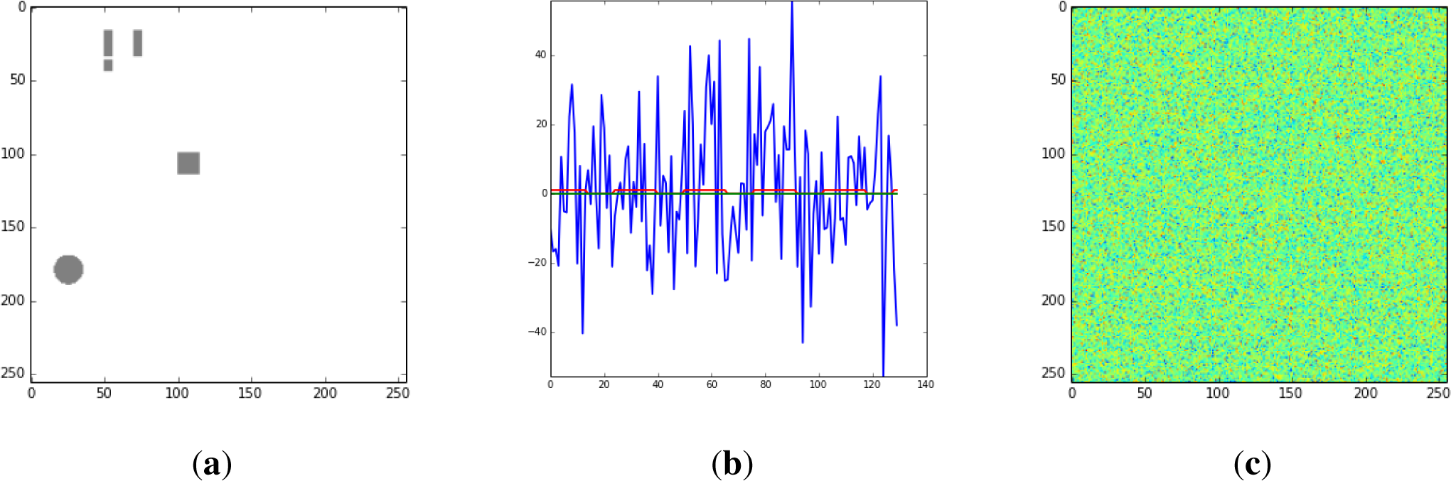
The simulated experiments consist of a sequence of active and rest periods where a number of images Tact, Trest are collected. This is repeated Nrep times. Figures 2–7 essentially tell the story. A few small regions, shown in Figure 2a are active. The fMRI simulated data is built by multiplying, for each pixel, the activity and the periodic hemodynamic response function and corrupting by the addition of noise. A typical pixel time series from the active region is shown in Figure 2b and one data image from an active period is shown in Figure 2c. The likelihood in Equation (21) shows that the corrupting Gaussian noise is assumed in the reconstruction, but the experimental noises could be of other types, so Gaussian and Cauchy noise are considered in the corruption of the data and Gaussian noise is always considered in this reconstruction in this paper. If some additional information about the noise becomes available, the method can be adapted accordingly.
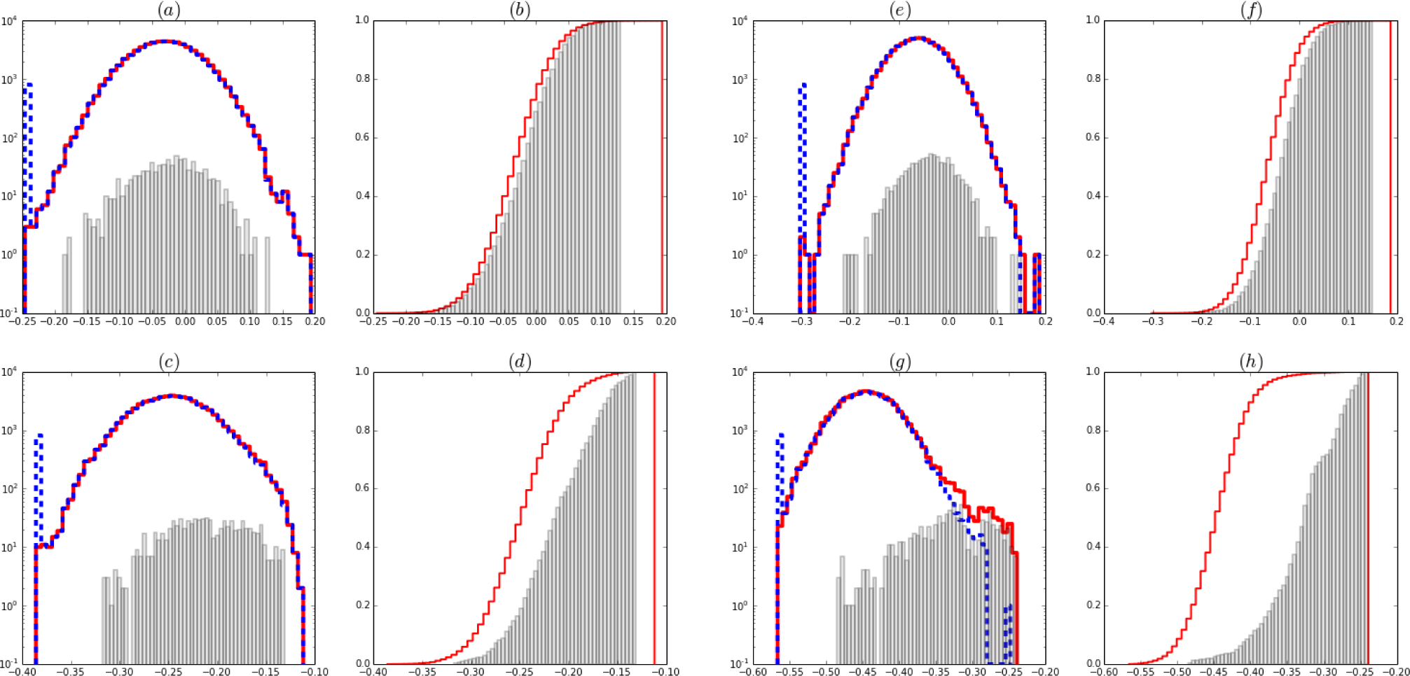
The numerical simulations shown here correspond to a brutal corruption with noise. For example, in Figure 3, the on-off hemodynamic function is of amplitude one and the Gaussian noise variance is 15, a signal to noise ratio of SNR= −23dB. The pure Bayes method (see Figures 3g,h) fails to identify the active regions, while the backward renormalization iteration leads to a rough identification of at least some active areas. The h field histograms help to understand the joint effect of the steps in the process. Note that the Bayes histograms, shown at the top of the left panel in Figures 4–6, are almost Gaussian. The renormalization transformation shifts the whole histogram to the origin, and the learning step Equation (27) shifts most fields to the left, where 〈Vd−1,IH〉 is small, and a few fields to the right, where it is large. This results in non-Gaussian distributions as shown at the bottom of the left panel in Figures 4–6. The meaning of the bumps is very interesting. Since these are simulations, the effects on the signal (active pixels) can be analyzed separately from the noise (inactive pixels) and this is clearly shown in the right hand side histograms of these figures. Since the active area is very small, the signal histogram is difficult to see. The shift in the signal histogram, relative to the whole picture field histogram is clearly seen even for the Bayes. But the shift is not large enough to escape the noise histogram umbrella. In the bottom pictures of the right panels in Figures 4–6, the signal histogram can be seen escaping the noise histogram and in breaking away making a bump in the otherwise Gaussian histograms. But this bump can be seen in the histogram of the fields of the whole image, signaling where to draw the line in deciding what is noise and what is signal. The same behavior can be seen in Figure 7, where the noise corruption is not Gaussian but Cauchy.
4.1. The Effect of the Lattice
It is due to the structure of the square renormalized lattices that the images of the active regions tend to show sharp horizontal or vertical edges. In order to get rid of this bias, an average of the magnetizations obtained with different choices of the origin of the lattice was performed. This was done by repeating the calculation Ls × Ls times, with the origin of the lattice at a position translated by (x, y) pixels, with 0 ≤ x, y < Ls. For each one the magnetization given by Equation (17), is calculated and then averaged at each pixel. Figures 8 and 9 show the results for L = 28 and Ls = 32. It can be seen that the sharp edges are smoothed by the averaging process leading to a better image.
Once the shift-averaged magnetization is available it can be used for instance to infer the form of the hemodynamic response function by doing a spatial average of the data time series over the region that has been identified as active [11]:
where Θ(x) = 0 or 1 if x < 0 or x ≥ 0 respectively and the threshold m0 can be obtained from the onset of the shoulder of the histogram (see Figure 8g). HRF (t), the spatial average over the active regions and B(t) the baseline, the spatial average over the regions identified as inactive, are shown in Figure 10a.
5. Discussion
The use of data to inform the prior is not new since Empirical Bayes (EB), e.g., see [12], has been around in many flavors for many decades, The idea behind the method presented here is different in at least two aspects. First, in EB the estimates of hyperparameters is made using the marginals of the data and the resulting posteriors of the sources are conditioned on estimates of the hyperparameters. In this sense a multigrid approach would be more aligned with the EB approach [12]. Second, the source variables in different lattices are related by renormalization and are not in the same footing as hyperparameters.
What are the main ingredients a problem has to satisfy so that the backward renormalization helps the inferential process? A method that builds priors that lead to better results has to introduce the use of some form of information that is not used in the pure Bayes. The new information is that the active regions are not isolated pixels but have some spatial extension. The data in the fMRI models come in two types of time series. One, the noise, has a mean value µn = 0 and the other has a mean value µs ≠ 0, the active pixels. In the simulations, Section 4, µs ∼ 1 and the variance of the noise ξ is taken up to σ ∼ 20 and still a partial identification of the active areas is possible. The renormalization of the data by blocking leads to a decrease in the effective variance
, where R2 is the typical area of the active regions and Ta the number of images where there is activity. For the pure Bayes approach the effective noise variance is only reduced by
. Blocking reduces the spatial resolution, which is recovered by the Backward renormalization step and the use of a more refined version of the data. This argument suggests that the large regions of activity will be more easily detected than the small regions as indeed happens in the simulations. Also the quality of recovery of a region of size R can not be expected to be better than that with pure Bayes at a variance 1/R times smaller. On the other hand, the inactive area is much larger than the active (about 7% of the total image shown in Figure 2 is active). This means that the identification of the inactive areas will be very effective translating into very few false positives. The backward renormalization step determines an effective transmission of the information to higher resolutions. Independently of the starting point, the pair interaction is driven to the critical value (in this case K ≈ .03) by the Backward renormalization step.
In Figure 10b, the receiver operating characteristic (ROC) curves are shown for different values of σ for both methods. The lines are obtained by measuring the specificity (T N/(F P + T N)) and the sensitivity (T P/(T P + F N)) when the magnetization threshold m0 is changed ((T, F) =(true, false), (P, N) = (positive, negative)). Note that the ROC curve for the pure Bayes with σ = 5 is approximately the same as for BRG priors with σ = 23, compatible with the discussion above for R = 4 or 5, a reasonable estimate, as seen in Figure 2.
In this simple case, the magnitude of the HRF is the same in every active region. But HRF amplitudes may vary in space in experimental cases. It is not difficult to include this variability in the model, e.g., see [11]. If this variation is permitted the pair interaction will also be driven by the data to space dependent values.
6. Conclusion
In this paper, the information used to construct priors is essentially that the sources are spatially localized but that single site activity is not the rule. The computational demands can be very much reduced if the starting point of an iterative process, like the Variational Bayes, is close to the final solution. The building of better priors through the building of more spatially refined lattices leads to simple problems at each new scale. The method presented here has several potential application scenarios. That a simulation of fMRI was chosen to exemplify the method is due to the simplicity and importance of the task-based or stimulus driven rest-active experimental paradigm. Applications to EEG/MEG source determination, and Connectome information flow will be presented elsewhere. We have not strived to present an extremely realistic simulation, but note that that doesn’t make it simpler. Noise to signal ratios in the simulations results presented here are very high and attest to the potential of the method. Even the error of corrupting with very high Cauchy noise and analyzing under the assumption that the noise was Gaussian could be handled quite efficiently. The Renormalization Group is one of the most important developments in Physics in the second half of the last century. It is typically used to integrate out degrees of freedom associated to the finer scales degrees of freedom. But here the reverse direction was taken. Typically the RG is referred to as a semigroup. But that applies only if the issue is how to go from the dynamical variables from one lattice to another. Then only the direction towards the coarser lattices is possible. However, if only the hyperparameters are considered then the RG is invertible. The hyperparameters or coupling constants, from one scale are related to the other scales and by inverting the RG map, the posterior in one scale feeds the prior in the next refinement. The use of the Migdal-Kadanoff renormalization group is not essential since there are several other possibilities for Ising variables. In general, the nature of the sources will dictate the renormalization group transformation useful to transport information from a coarse to a finer lattice. In addition, the choice of the type of lattice can be very important. Each application will have its own peculiarities, but in all of them, the choice of the prior at the coarsest spatial representation will be quite irrelevant.
Acknowledgments
I thank Ariel Caticha for discussions about Entropic Inference; Said Rabbani, Selene Amaral, Leonardo Barbosa and Leonardo Tavares for discussions about multigrid priors; Felippe Alves Pereira for his help with the python code. The author received support from the Núcleo de Apoio à Pesquisa CNAIPS of the University of São Paulo.
Conflicts of Interest
The author declares no conflict of interest.
References
- Wilson, K.G. The Renormalization Group and Critical Phenomena. Rev. Mod. Phys 1983, 55, 583–600. [Google Scholar]
- Goodman, J.; Sokal, A.D. Multigrid Monte Carlo Method. Conceptual Foundations. Phys. Rev. D 1989, 40, 2035–2071. [Google Scholar]
- Amaral, R.; Rabbani, S.R.; Caticha, N. Multigrid Priors for a Bayesian Approach to FMRI. NeuroImage 2004, 23, 654–662. [Google Scholar]
- Giffin, A.; Caticha, A. Updating Probabilities with Data and Moments. Presented at the 27th Interenational Workshop on Bayesian Inference and Maximum Entropy Methods in Science and Engineering, Saratoga Springs, NY, USA, 8–13 July 2007. [CrossRef]
- Bishop, C.M. Pattern Recognition and Machine Learning, 1st ed; Information Science and Statistics Series; Springer: New York, NY, USA, 2007. [Google Scholar]
- Logothetis, N.K. What We Can Do and What We Cannot Do with FMRI. Nature 2008, 453, 869–878. [Google Scholar]
- Ashby, F.G. Statistical Analysis of FMRI Data; MIT Press: Hong Kong, China, 2011. [Google Scholar]
- Migdal, A.A. Phase transitions in gauge and spin-lattice systems. Sov. Phys. JETP 1975, 42, 743–746. [Google Scholar]
- Kadanoff, L.P. Notes on Migdal’s Recursion Formulas. Ann. Phys 1976, 100, 359–394. [Google Scholar]
- Griffiths, R.B.; Kaufman, M. Spin Systems on hierarchical lattices. Introduction and thermodynamic limit. Phys. Rev. B 1982, 26, 5022–5032. [Google Scholar]
- Amaral, R.; Rabbani, S.R.; Caticha, N. BOLD Response Analysis by Iterated Local Multigrid Priors. Neuroimage 2006, 36, 361–369. [Google Scholar]
- Carlin, B.P.; Louis, T.A. Bayes and Empirical Bayes methods for Data Analysis; Chapman and Hall/CRC: Boca Raton, Florida, USA, 1996. [Google Scholar]
Figure 1.
The Migdal Kadanoff Backward Renormalization Group flow.

Figure 2.
(a): Active areas, without noise. (b): An active pixel times series is a square periodic hemodynamic function with amplitude 1 or zero (red) plus Gaussian noise with σdata(= 20) (blue). (c): A typical simulated data image during the active period. Active time Tact = 14, resting time Trest = 12, number of active-rest repetitions Nrep = 5. Time units: one image per unit.

Figure 3.
(a–e) Contour plots and Backward Renormalization hyperparameters hd(i) for lattices L × L, L = 2d, d = 3 − 7 (positive values in red, negative values in blue).(f) Final result for lattice with d = 8, which shows the threshold image of the fields. The threshold is chosen from the histogram of Figure 6. (g) Pure Bayes field contour plot and (h) field. Data corrupted with Gaussian noise with σ = 15.
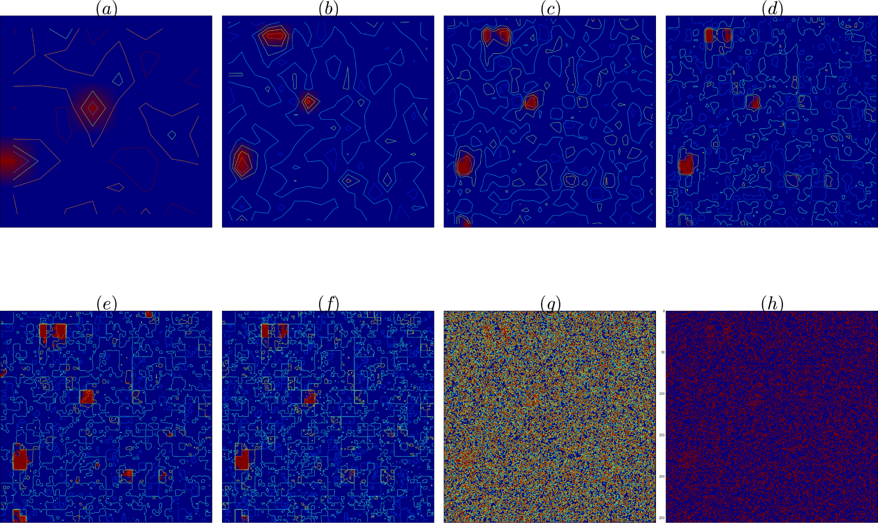
Figure 4.
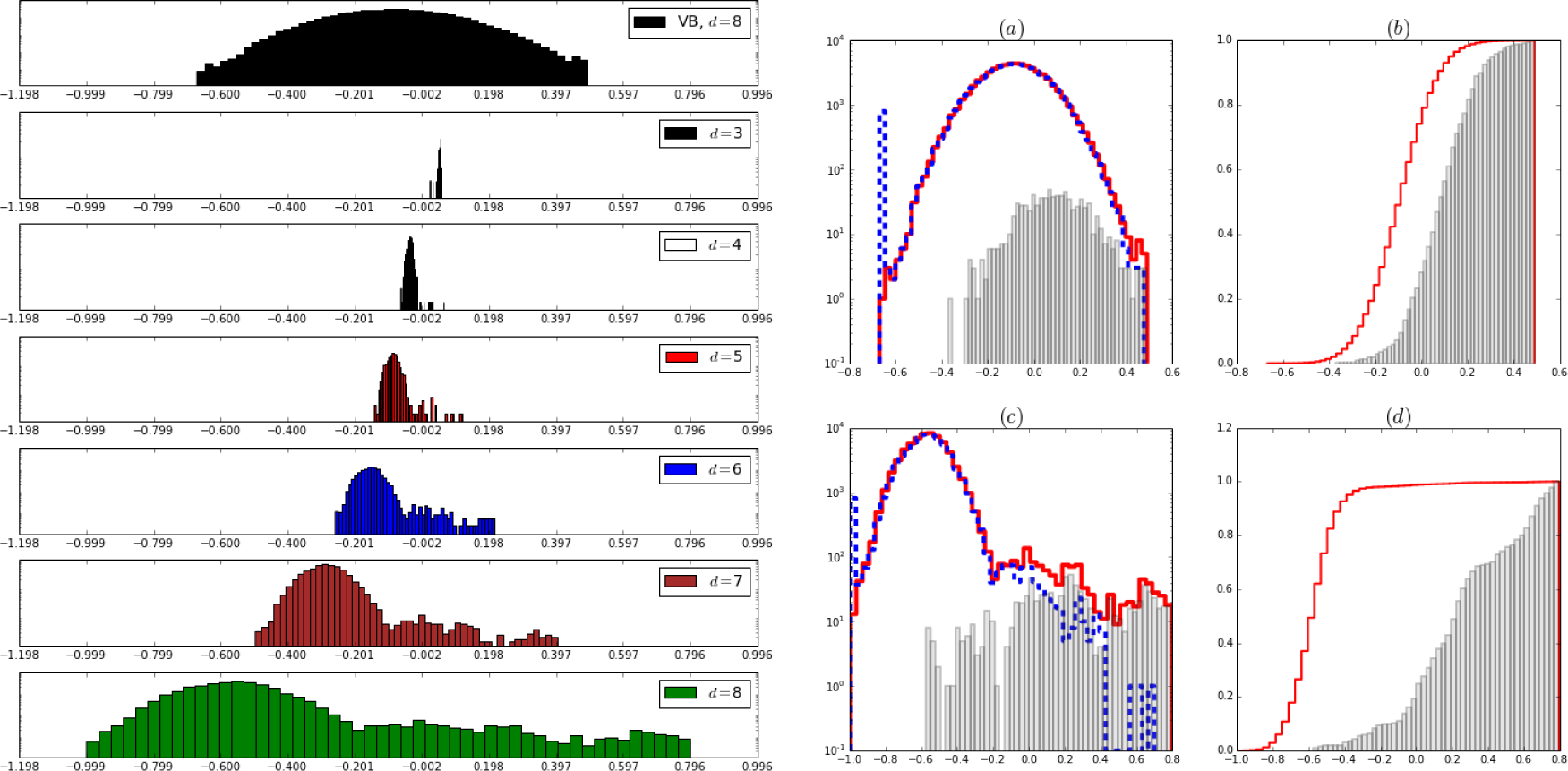
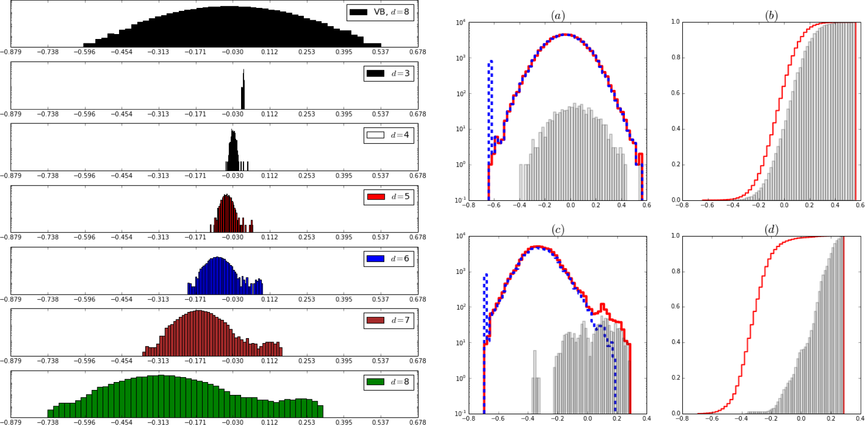
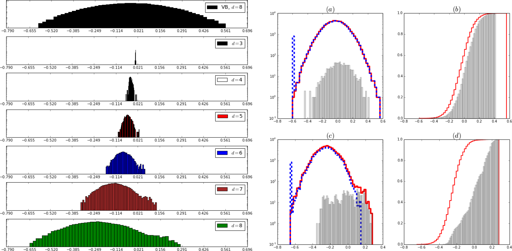
Left panel: Normalized histograms of the magnetic fields hyperparameters hi. Vertical axis in log scale. From top to bottom, first figure shows the Gaussian like Bayes results for the full lattice. Second to seventh figures show the histograms for the BRG priors as the lattice side increases from 23 to 28. Note that the inverse renormalization (Equations (15)) sends the distribution to the left towards lower values of the field. The learning step (Equations (27)) send most values to the left but a few to the right, hence the distributions become bimodal, separating noise from signal. Right panel, (a) and (c): The normalized histograms hi in logarithmic scale. Steps (red): whole image. Dashed lines (blue): only from the region known to be inactive in the simulation. Bars (grey): from the region known to be active in the simulation. Right (b) and (d): cumulative histograms. Steps (red): Whole image. Bars (grey): the active regions. Top row ((a) and (b): Bayes. Bottom row ((c) and (d)): final result of the BRG priors in L × L lattice, L = 28. Data corrupted with Gaussian noise with σ = 7
Figure 4.
Left panel: Normalized histograms of the magnetic fields hyperparameters hi. Vertical axis in log scale. From top to bottom, first figure shows the Gaussian like Bayes results for the full lattice. Second to seventh figures show the histograms for the BRG priors as the lattice side increases from 23 to 28. Note that the inverse renormalization (Equations (15)) sends the distribution to the left towards lower values of the field. The learning step (Equations (27)) send most values to the left but a few to the right, hence the distributions become bimodal, separating noise from signal. Right panel, (a) and (c): The normalized histograms hi in logarithmic scale. Steps (red): whole image. Dashed lines (blue): only from the region known to be inactive in the simulation. Bars (grey): from the region known to be active in the simulation. Right (b) and (d): cumulative histograms. Steps (red): Whole image. Bars (grey): the active regions. Top row ((a) and (b): Bayes. Bottom row ((c) and (d)): final result of the BRG priors in L × L lattice, L = 28. Data corrupted with Gaussian noise with σ = 7

Figure 5.
Same as Figure 4, data corrupted with Gaussian noise with σ = 15.
Figure 5.
Same as Figure 4, data corrupted with Gaussian noise with σ = 15.

Figure 6.
Same as Figure 4, data corrupted with Gaussian noise with σ = 20. The images corresponding to this histograms are shown in Figure 3.

Figure 7.
Normalized histograms of the magnetic fields hi. Data corrupted with Cauchy noise with amplitude at half width σC = 20 (figures a-d) and σC = 10 (figures e-h). Images (a, b, e, f) are the histograms for the Bayes algorithm and (c,d,g,h) for the BRG priors. Note first that for the case σC = 10 the histogram in figure (g) develops a shoulder, consistent with the fact that a partial identification of the active areas is possible. The other cases (a, c, e) fail to develop a shoulder and the methods can’t identify the active areas. Figure (g) shows that even though the noise was Cauchy and the data analysis done under the hypothesis of Gaussian noise, the BRG priors can partially find the active areas. Continuous steps (red): full image. Dashed steps (blue) inactive regions. Bars (grey) histogram of hi of Active regions.

Figure 8.
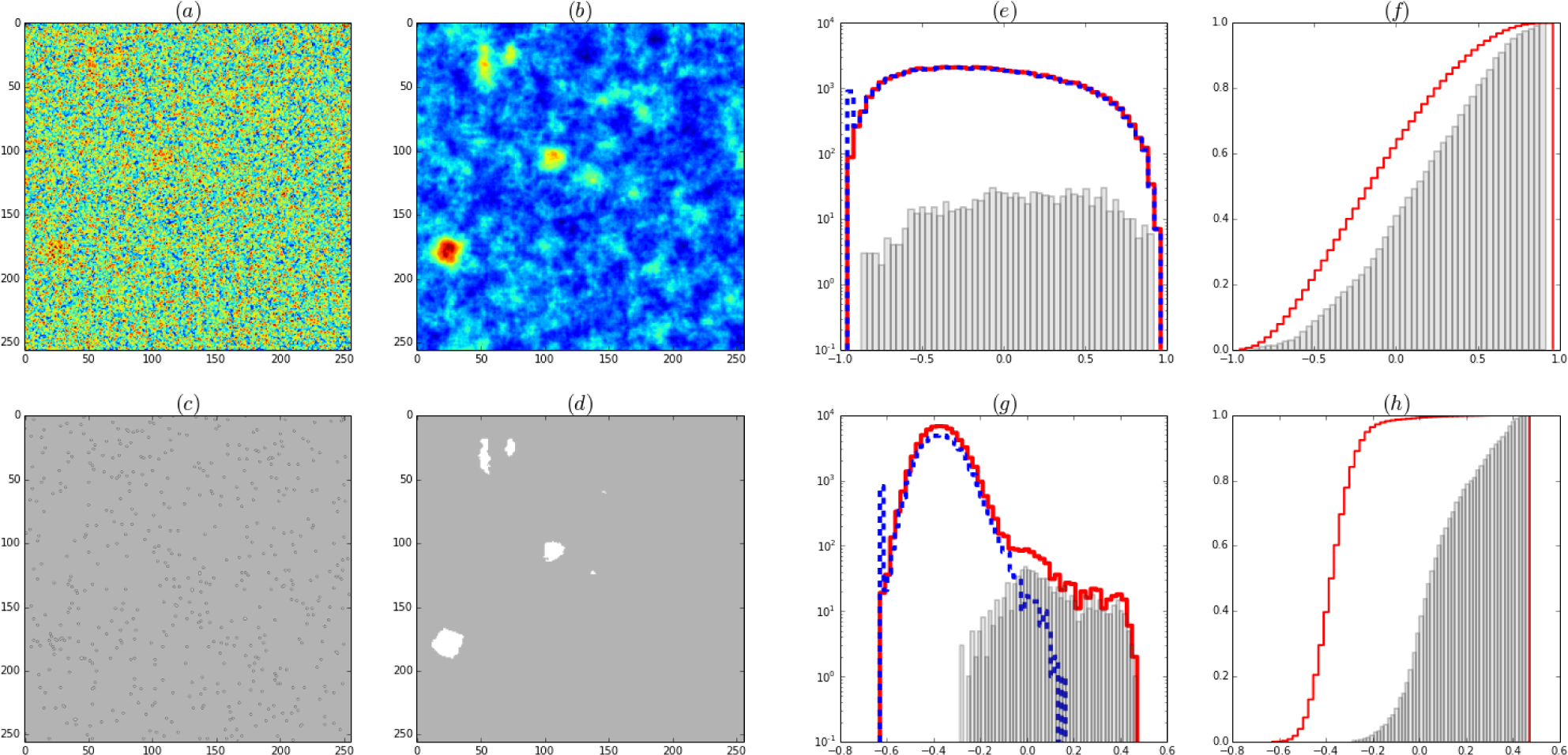
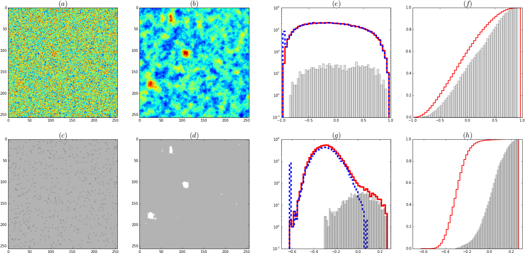
Magnetization or expected value of activity for σ = 15. (a) Pure Bayes, (b) BRG priors: Average of Ls × Ls shifts with Ls = 32. Thresholded magnetization for (c) Pure Bayes (d) BRG priors. (e-f) Normalized histograms of the magnetization. (e) and (f)(cumulative) Pure Bayes, (g) and (h) Normalized histograms (cumulative) BRG priors. In continuous line (red) the magnetization of the full image, in dashed line (blue) the histogram of the inactive region, in (grey) bars the histograms of the region where there is activity. The full histogram is experimentally available. The separation into signal (bars) and noise (dashed) can only be done in the simulation. The thresholds of (c) and (d) are chosen to give the same number of active sites. The threshold for figure (d) is chosen at the beginning of the shoulder in the continuous histogram in figure (g).
Figure 8.
Magnetization or expected value of activity for σ = 15. (a) Pure Bayes, (b) BRG priors: Average of Ls × Ls shifts with Ls = 32. Thresholded magnetization for (c) Pure Bayes (d) BRG priors. (e-f) Normalized histograms of the magnetization. (e) and (f)(cumulative) Pure Bayes, (g) and (h) Normalized histograms (cumulative) BRG priors. In continuous line (red) the magnetization of the full image, in dashed line (blue) the histogram of the inactive region, in (grey) bars the histograms of the region where there is activity. The full histogram is experimentally available. The separation into signal (bars) and noise (dashed) can only be done in the simulation. The thresholds of (c) and (d) are chosen to give the same number of active sites. The threshold for figure (d) is chosen at the beginning of the shoulder in the continuous histogram in figure (g).

Figure 9.
Same as Figure 8 but σ = 20.
Figure 9.
Same as Figure 8 but σ = 20.

Figure 10.
(a) Hemodynamic response as a function of time. Dashed line (Red) the active-inactive task. Thick line (Blue) HRF (t), the data spatial average over active region. Thin line (Green) the baseline B(t), the data spatial average over the inactive sites. BRG priors-shifted average algorithm. Spatial averages over regions where local magnetization is higher than threshold (experimentally available from the onset of the shoulder of Figure 5 Right.(c)). Data corrupted with Gaussian noise with σ = 15. Range of Shift of Lattice origin = 32 × 32. The times series shown are smoothed using a moving-average with a window of 5 time steps. (b) ROC curves, 1− Specificity vs Sensitivity, obtained by changing the magnetization threshold for activity, BRG priors are shown in continuous lines, Pure Bayes in dashed lines. (c) The statistics t = (mf −ms)/max(var mf, var ms) measures the separability of two distributions of magnetization as a function of the magnitude of the corrupting noise: mf of the full picture and ms of the active region.

© 2015 by the authors; licensee MDPI, Basel, Switzerland This article is an open access article distributed under the terms and conditions of the Creative Commons Attribution license (http://creativecommons.org/licenses/by/4.0/).
Share and Cite
MDPI and ACS Style
Caticha, N. Source Localization by Entropic Inference and Backward Renormalization Group Priors. Entropy 2015, 17, 2573-2589. https://doi.org/10.3390/e17052573
AMA Style
Caticha N. Source Localization by Entropic Inference and Backward Renormalization Group Priors. Entropy. 2015; 17(5):2573-2589. https://doi.org/10.3390/e17052573
Chicago/Turabian StyleCaticha, Nestor. 2015. "Source Localization by Entropic Inference and Backward Renormalization Group Priors" Entropy 17, no. 5: 2573-2589. https://doi.org/10.3390/e17052573