
Information Geometry on Complexity and Stochastic Interaction

1
Max Planck Institute for Mathematics in the Sciences, Inselstraße 22, 04103 Leipzig, Germany
2
Faculty of Mathematics and Computer Science, University of Leipzig, PF 100920, 04009 Leipzig, Germany
3
Santa Fe Institute, 1399 Hyde Park Road, Santa Fe, NM 87501, USA
Entropy 2015, 17(4), 2432-2458; https://doi.org/10.3390/e17042432
Submission received: 28 February 2015
/
Revised: 2 April 2015
/
Accepted: 8 April 2015
/
Published: 21 April 2015
(This article belongs to the Special Issue Information Theoretic Incentives for Cognitive Systems)
Abstract
:Interdependencies of stochastically interacting units are usually quantified by the Kullback-Leibler divergence of a stationary joint probability distribution on the set of all configurations from the corresponding factorized distribution. This is a spatial approach which does not describe the intrinsically temporal aspects of interaction. In the present paper, the setting is extended to a dynamical version where temporal interdependencies are also captured by using information geometry of Markov chain manifolds.
1. Preface: Information Integration and Complexity
Since the publication of Shannon’s pioneering work in 1948 [1], it has been hypothesized that his information theory provides means for understanding information processing and learning in the brain. Already in the 1950s, the principle of redundancy reduction has been proposed independently by Attneave [2] and Barlow [3]. In 1981, Laughlin has provided some experimental evidence for the redundancy reduction principle in terms of the maximization of the output entropy of large monopolar cells of the fly’s compound eye [4]. As only deterministic response functions have been considered, this principle turns out to be equivalent to the mutual information maximization between the input and the output. Later, Linsker [5] has demonstrated that the maximization of mutual information in a layered feed-forward network leads to feature detectors that are similar to those observed by Hubel and Wiesel in the visual system of the cat and the monkey [6,7]. He coined his information-theoretic principle of learning the infomax principle.
The idea that an information-theoretic principle, such as the infomax principle, governs learning processes of neuronal systems has attracted many researchers. A highly recognized contribution in this regard is the work by Bell and Sejnowski [8] which applies the infomax principle to the source separation problem. An exhaustive review of all relevant contributions to that field is not within the scope of this short discussion. I shall focus on approaches that aim at relating such information based principles to the overall complexity of the system. In particular, I shall concentrate on the theory of information integration and complexity, initially proposed by Tononi, Sporns, and Edelman [9], and further developed and analyzed in a series of papers [10–15]. I shall compare this line of research with my own information-geometric approach to complexity, initially proposed in my manuscript [16], entitled Information Geometry on Complexity and Stochastic Interaction, which led to various lines of research that I am going to outline below. This manuscript constitutes the main body of the present paper, starting with Section 2. It quantifies complexity as the extent to which the whole is more than the sum of its parts using information geometry [17]. Thereby, it extends the notion of multi-information [18,19], also called information integration in [9], to the setting of discrete time stochastic processes, in particular Markov chains. This article was originally accepted for publication in IEEE Transactions on Information Theory, subject to minor revision. However, by the end of the unusually long reviewing process I had come to the conclusion that my geometric approach has to be further improved in order to address important aspects of complexity (I shall be more concrete on that). Recent developments, on the other hand, suggest that this work is of relevance in the context of information integration already in its present form [12–15,20,21]. Therefore, it should be useful to provide it together with a discussion of its strengths and shortcomings, thereby relating it to similar work that has been developed since its first publication.
Let us first consider the so-called multi-information [18,19] of a random vector X = (Xv)v∊V, taking values in a finite set:
where H denotes the Shannon entropy (we assume V to be a non-empty and finite set). The multi-information vanishes if and only if the variables Xv, v ∊ V, are stochastically independent. In their original paper [9], Tononi, Sporns, and Edelman call this quantity integration. Following their intuition, however, the notion of integration should rather refer to a dynamical process, the process of integration, which is causal in nature. In later works, the dynamical aspects have been more explicitly addressed in terms of a causal version of mutual information, leading to improved notions of effective information and information integration, denoted by Φ [10,11]. In fact, most formulated information-theoretic principles are, in some way or another, based on (conditional) mutual information. This directly fits into Shannon’s classical sender-receiver picture [1], where the mutual information has been used in order to quantify the capacity of a communication channel. At first sight, this picture suggests to treat only feed-forward networks, in which information is transmitted from one layer to the next, as in the context of Linsker’s infomax principle. In order to overcome this apparent restriction, however, we can simply unfold the dynamics in time and consider corresponding temporal information flow measures, which allows us to treat also recurrent networks. In what follows, I am going to explain this idea in more detail, thereby providing a motivation of the quantities that are derived in Section 2 in terms of information geometry.
We consider again a non-empty and finite set V of nodes and assume that each v ∊ V receives signals from a set of nodes which we call parents of v and denote by pa(v). Based on the received signals, the node v updates its state according to a Markov kernel K(v), the mechanism of v, which quantifies the conditional probability of its new state
given the current state ωpa(v) of its parents. If v ∊ pa(v), this update will involve also ωv for generating the new state
. How much information is involved from “outside”, that is from ∂(v) := pa(v) \ v, in addition to the information given by ωv? We can define the local information flow from this set as
where MI stands for the (conditional) mutual information. Note that this is the uncertainty reduction that the node v gains through the knowledge of its parents’ state, in addition to its own state. Now let us define the total information flow in the network. In order to do so, we have to consider the overall transition kernel. Because the nodes update their states in parallel, the global transition kernel is given as
In order to quantify the total information flow in the network, we simply add all the local information flows, defined by Equation (2), and obtain
It is easy to see that the total information flow vanishes whenever the global transition kernel has the following structure which encodes the dynamics of isolated non-communicating nodes:
Referring to these kernels as being split, we are now ready to give our network information flow measure, defined by Equation (4), a geometric interpretation. If K has the structure Equation (3) then
Here, Dp(K || K′) is a measure of “distance”, in terms of the Kullback-Leibler divergence, between K and K′ with respect to the distribution p (see definition by Equation (23)). The expression on the right-hand side of Equation (6) can be considered as an extension of the multi-information (1) to the temporal domain. The second equality, Equation (7), gives the total information flow in the network a geometric interpretation as the distance of the global dynamics K from the set of split dynamics. Stated differently, the total information flow can be seen as the extent to which the whole transition X → X′ is more than the sum of its individual transitions
, v ∊ V. Note, however, that Equation (6) follows from the additional structure (3) which implies
. This structure encodes the consistency of the dynamics with the network. Equation (7), on the other hand, holds for any transition kernel K. Therefore, without reference to a particular network, the distance minK′ split Dp(K || K′) can be considered as a complexity measure for any transition X → X′, which we denote by C(1)(X → X′). The information-geometric derivation of C(1)(X → X′) is given in Section 2.4.1. Restricted to kernels that are consistent with a network, the complexity C(1)(X → X′) reduces to the total information flow in the network (see Proposition 2 (iv)).
In order to consider the maximization of the complexity measure C(1)(X → X′) as a valid information-theoretic principle of learning in neuronal systems, I analyzed the natural gradient field on the manifold of kernels that have the structure given by Equation (3) (see [17,22] for the natural gradient method within information geometry). In [23] I proved the consistency of this gradient in the sense that it is completely local: If every node v maximizes its own local information flow, defined by Equation (2), in terms of the natural gradient, then this will be the best way, again with respect to the natural gradient, to maximize the complexity of the whole system. This suggests that the infomax principle by Linsker and also Laughlin’s ansatz, applied locally to recurrent networks, will actually lead to the maximization of the overall complexity. We used geometric methods to study the maximizers of this complexity analytically [24,25]. We have shown that they are almost deterministic, which has quite interesting implications, for instance for the design of learning systems that are parametrized in a way that allows them to maximize their complexity [26] (see also [27] for an overview of geometric methods for systems design). Furthermore, evidence has been provided in [25] that the maximization of C(1)(X → X′) is achieved in terms of a rule that mimics the spike-timing-dependent plasticity of neurons in the context of discrete time. Together with Wennekers, we have studied complexity maximization as first principle of learning in neural networks also in [28–33].
Even though I implicitly assumed that a natural notion of information flow has to reflect the causal interactions of the nodes, I should point out that the above definition of information flow has a shortcoming in this regard. If Xv and X∂(v) contain the same information, due to a strong stochastic dependence, then the conditional mutual information in Equation (2) will vanish, even though there might be a strong causal effect of ∂(v) on v. Thus, correlation among various potential causes can hide the actual causal information flow. The information flow measure of Equation (2) is one instance of the so-called transfer entropy [34] which is used within the context of Granger causality and has, as a conditional mutual information, the mentioned shortcoming also in more general settings (see a more detailed discussion in [35]). In order to overcome these limitations of the (conditional) mutual information, in a series of papers [35–39] we have proposed the use of information theory in combination with Pearl’s theory of causation [40]. Our approach has been discussed in [41] where a variant of our notion of node exclusion, introduced in [36], has been utilized for an alternative definition. This definition, however, is restricted to direct causal effects and does not capture, in contrast to [35], mediated causal effects.
Let us now draw a parallel to causality issues of the complexity measure introduced in the original work [9], which we refer to as TSE-complexity. In order to do so, consider the following representation of the original TSE-complexity as weighted sum of mutual informations:
where
. Interpreting the mutual information between A and its complement V\A in this sum as an information flow is clearly misleading. These terms are completely associational and neglect the causal nature of information flow. In [10,11], Tononi and Sporns avoid such inconsistencies by injecting noise (maximum entropy distribution) into A and then measuring the effect in V \ A. They use the corresponding interventional mutual information in order to define effective information. Note that, although their notion of noise injection is conceptually similar to the notion of intervention proposed by Pearl, they formalize it differently. However, the idea of considering a post-interventional mutual information is similar to the one formalized in [35,36] using Pearl’s interventional calculus.
Clearly, the measure C(1)(X → X′) does not account for all aspects of the system’s complexity. One obvious reason for that can be seen by comparison with the multi-information, defined by Equation (1), which also captures some aspects of complexity in the sense that it quantifies the extent to which the whole is more than the sum of its elements (parts of size one). On the other hand, it attains its (globally) maximal value, if and only if the nodes are completely correlated. Such systems, in particular completely synchronized systems, are generally not considered to be complex. Furthermore, it turns out that these maximizers are determined by the marginals of size two [42]. Stated differently, the maximization of the extent to which the whole is more than the sum of its parts of size one leads to systems that are not more than the sum of their parts of size two (see for a more detailed discussion [43,44]). Therefore, the multi-information does not capture the complexity of a distribution at all levels. The measure C(1)(X → X′) has the same shortcoming as the multi-information. In order to study different levels of complexity, one can consider coarse-grainings of the system at different scales in terms of corresponding partitions Π = {S1,…, Sn} of V. Given such a partition, we can define the information flows among its atoms Si as we already did for the individual elements v of V. For each Si, we denote the set of nodes that provide information to Si from outside by
. We quantify the information flow into Si as in Equation (2):
For a transition that satisfies Equation (3), the total information flow among the parts Si is then given by
We can now define the Π-complexity of a general transition, as we already did for the complete partition:
Obviously, the Π-complexity coincides with the information flow IF (X → X′ | Π) in the case where the transition kernel is compatible with the network. The information-geometric derivation of C(X → X′ | Π) is given in Section 2.4.1. In the early work [10,11], a similar approach has been proposed where only bipartitions have been considered. Later, an extension to arbitrary partitions has been proposed by Balduzzi and Tononi [12,13] where the complexity defined by Equation (11) appears as measure of effective information. Note, however, that there are important differences. First, the proposed measure by Tononi and his coworkers is reversed in time, so that their quantity is given by Equation (11) where X and X′ have exchanged roles. This time-reversal of the effective information is motivated by its intended role as a measure relevant to conscious experience. This does not make any difference in the case where a stationary distribution is chosen as input distribution. However, in order to be consistent with causal aspects of conscious experience, the authors choose a uniform input distribution, which models the least informative prior about the input.
Note that there is also a closely related measure, referred to as synergistic information in the works [15,45]:
The last equation directly follows from Proposition 1 (iii) (see the derivation of Equation (29)). Interpreting the mutual informations as (one-step) predictive information [46–48], the synergistic information quantifies the extent to which the predictive information of the whole system exceeds the sum of predictive informations of the elements.
Now, having for each partition of the system the corresponding Π-complexity of Equation (11), how should one choose among all these complexities the right one? Following the proposal made in [10–13], one should identify the partition (or bipartition) that has the smallest, appropriately normalized, Π-complexity. Although the overall complexity is not explicitly defined in these works, the notion of information integration, denoted by Φ, seems to directly correspond to it. This is confirmed by the fact that information integration is used for the identification of so-called complexes in the system. Loosely speaking, these are defined to be subsets S of V with maximal information integration Φ(S). This suggests that the authors equate information integration with complexity. In a further refinement [12,13] of the information integration concept, this is made even more explicit. In [13], Tononi writes: “In short, integrated information captures the information generated by causal interactions in the whole, over and above the information generated by the parts.”
Defining the overall complexity simply as the minimal one, with respect to all partitions, will ensure that a complex system has a considerably high complexity at all levels. I refer to this choice as the weakest link approach. This is not the only approch to obtain an overall complexty measure from individual ones defined for various levels. In order to give an instructive example for an alternative approach, let us highlight another representation of the TSE-complexity. Instead of the atoms of a partition, this time we consider the subsets of V with a given size k ∊ {1,…, N} and define the following quantity:
Let us compare this quantity with the multi-information of Equation (1). For k = 1, they are identical. While the multi-information quantifies the extent to which the whole is more than the sum of its elements (subsets of size one), its generalization C(k)(X) can be interpreted as the extent to which the whole is more than the sum of its parts of size k. Now, defining the overall complexity as the minimal C(k)(X) would correspond to the weakest link approach which I discussed above in the context of partitions. A complex system would then have considerably high complexity C(k)(X) at all levels k. However, the TSE-complexity is not constructed according to the weakest link approach, but can be written as a weighted sum of the terms C(k)(X):
where
. The right choice of the weights is important here. I refer to this approach as the average approach. Clearly, one can interpolate between the weakest link approach and the average approach using the standard interpolation between the L∞-norm (maximum) and the L1-norm (average) in terms of the Lp-norms, p ≥ 1. However, Lp-norms appear somewhat unnatural for entropic quantities.
The TSE-complexity has also an information-geometric counterpart which has been developed in a series of papers [43,44,49,50]. It is instructive to consider this geometric reformulation of the TSE-complexity. For a distribution p, let p(k) be the maximum-entropy estimation of p with fixed marginals of order k. In particular, p(N) = p, and p(1) is the product of the marginals pv, v ∊ V, of order one. In some sense, p(k) encodes the structure of p that is contained only in the parts of size k. The deviation of p from p(k) therefore corresponds to C(k)(X), as defined in Equation (14). This correspondence can be made more explicit by writing this deviation in terms of a difference of entropies:
where D denotes the Kullback-Leibler divergence. If we compare the Equations (16) and (14), then we see that
corresponds to
. Indeed, both terms quantify the entropy that is contained in the marginals of order k. From the information-geometric point of view, however, the second term appears more natural. The first term seems to count marginal entropies multiple times so that we can expect that this mean value is larger than
. In [43], we have shown that this is indeed true, which implies
If we replace the C(k)(X) in the definition (15) of the TSE-complexity by D(p || p(k)), then we obtain with the Pythagorean theorem of information geometry the following quantity:
where
. Let us compare this with the multi-information. Following [18], we can decompose the multi-information as
I already mentioned that high multi-information is achieved for strongly correlated systems, which implies that the global maximizers can be generated by systems that only have pairwise interactions [42], that is p = p(2). It follows that in the above decompsition of Equation (19), only the first term D(p(2) || p(1)) is positive while all the other terms vanish for maximizers of the multi-information. This suggests that the multi-information does not weight all contributions D(p(k+1) || p(k)) to the stochastic dependence in a way that would qualify it as a complexity measure. The measure defined by Equation (18), which I see as an information-geometric counterpart of the TSE-complexity, weights the higher-order contributions D(p(k+1) || p(k)), k ≥ 2, more strongly. In this geometric picture, we can interpret the TSE-complexity as a rescaling of the multi-information in such a way that its maximization will emphasize not only pairwise interactions.
Concluding this preface, I compared two lines of research, the one pursued by Tononi and coworkers on information integration, and my own information-geometric research on complexity. The fact that both research lines independently identified closely related core concepts of complexity confirms that these concepts are quite natural. The comparison of the involved ideas suggests the following intuitive definition of complexity: The complexity of a system is the extent to which the whole is more than the sum of its parts at all system levels. I argue that information geometry provides natural methods for casting this intuitive definition into a formal and quantitative theory of complexity. My paper [16], included here as Section 2, exemplifies this way of thinking about complexity. It is presented with only minor changes compared to its initial publication, except that the original reference list is replaced by the largely extended up-to-date list of references. This implies repetitions of a few standard definitions which I already used in this preface.
2. “Information Geometry on Complexity and Stochastic Interaction”, Reference [16]
2.1. Introduction
“The whole is more than the sum of its elementary parts.” This statement characterizes the present approach to complexity. Let us put it in a more formal setting. Assume that we have a system consisting of elementary units v ∊ V. With each non-empty subsystem S ⊂ V we associate a set
of objects that can be generated by S. Examples for such objects are (deterministic) dynamical systems, stochastic processes, and probability distributions. Furthermore, we assume that there is a “composition” map
that defines how to put objects of the individual units together in order to describe a global object without any interrelations. The image of ⊗ consists of the split global objects which are completely characterized by the individual ones and therefore represent the absence of complexity. In order to quantify complexity, assume that there is given a function D : (x, y) ↦ D(x || y), that measures the divergence of global objects x,
. We define the complexity of
to be the divergence from being split:
Of course, this approach is very general, and there are many ways to define complexity following this concept. Is there a canonical way? At least, within the probabilistic setting, information geometry [17,51] provides a very convincing framework for this. In the context of random fields, it leads to a measure for “spatial” interdependencies: Given state sets Ωv, v ∊ V, we define the set OS of objects that are generated by a subsystem S ⊂ V to be the probability distributions on the product set
. A family of individual probability distributions p(v) on Ωv can be considered as a distribution on the whole configuration set
by identifying it with the product
. In order to define the complexity of a distribution
on the whole system, according to Equation (20) we have to choose a divergence function. A canonical choice for D is given by the Kullback-Leibler divergence [52,53]:
The distributions with maximal interdependence (complexity) are given by
Spatial interdependence has been studied by Amari [18] and Ay [23,55] from the information-geometric point of view, where it is referred to as (stochastic) interaction and discussed in view of neural networks. The aim of the present paper is to use the concept of complexity that is formalized by Equation (20) in order to extend spatial interdependence to a dynamical notion of interaction, where the evolution in time is taken into account. Therefore, the term “stochastic interaction” is mainly used in the context of spatio-temporal interdependence.
The present paper is organized as follows. After a brief introduction into the information-geometric description of finite probability spaces in Section 2.2, the general notion of separability is introduced for Markovian transition kernels, and information geometry is used for quantifying non-separability as divergence from separability (Section 2.3). In Section 2.4, the presented theoretical framework is used to derive a dynamical version of the definition in Equation (21), where spatio-temporal interdependencies are quantified and referred to as stochastic interaction. This is illustrated by some simple but instructive examples.
2.2. Preliminaries on Finite Information Geometry
In the following, Ω denotes a non-empty and finite set. The vector space ℝΩ of all functions Ω → ℝ carries the natural topology, and we consider subsets as topological subspaces. The set of all probability distributions on Ω is given by
Following the information-geometric description of finite probability spaces, its interior
can be considered as a differentiable submanifold of ℝΩ with dimension |Ω|−1 and the basis-point independent tangent space
(If one considers
as an “abstract” differentiable manifold, there are many ways to represent it as a submanifold of ℝΩ. In information geometry, the natural embedding presented here is called (−1)-respectively (m)-representation)
With the Fisher metric 〈·,·〉p : T(Ω) × T(Ω) → ℝ in p ∊ defined by
becomes a Riemannian manifold [56] (In mathematical biology this metric is also known as Shahshahani metric [57]). The most important additional structure studied in information geometry is given by a pair of dual affine connections on the manifold. Application of such a dual structure to the present situation leads to the notion of (−1)- and (+1)-geodesics: Each two points p, q can be connected by the geodesics
, α ∊ {−1, +1, with
Here, r(t) denotes the normalization factor.
A submanifold ε of
is called an exponential family if there exist a point p0 ∊ and vectors v1,…, vd ∊ RΩ, such that it can be expressed as the image of the map
, θ = (θ1,…, θd) ↦ pθ, with
Let p be a probability distribution in
. An element p′∊ ε is called (−1)-projection of p onto ε iff the (−1)-geodesic connecting p and p′ intersects ε orthogonally with respect to the Fisher metric. Such a point p′ is unique ([51], Theorem 3.9, p. 91) and can be characterized by the Kullback-Leibler divergence [52,53] (This is a special case of Csiszár’s f-divergence [54])
We define the distance D(· || ε) :
from E by
It is well known that a point p′ ∊ ε is the (−1)-projection of p onto ε if and only if it satisfies the minimizing property D(p || ε) = D(p || p′) ([51], Theorem 3.8, p. 90; [17], Corollary 3.9, p. 63).
In the present paper, the set of states is given by the Cartesian product of individual state sets Ωv, v ∊ V, where V denotes the set of units. In the following, the unit set and the corresponding state sets are assumed to be non-empty and finite. For a subsystem S ⊂ V,
denotes the set of all configurations on S. The elements of
are the random fields on S. One has the natural restriction XS : ΩV → ΩS, ω = (ωv)v∊V ↦ ωS := (ωv)v∊S, which induces the projection
, p ↦pS, where pS denotes the image measure of p under the variable XS. If the subsystem S consists of exactly one unit v, we write pv instead of p{v}.
The following example, which allows us to put the definition of Equation (21) into the information-geometric setting, represents the main motivation for the present approach to stochastic interaction. It will be generalized in Section 2.4.
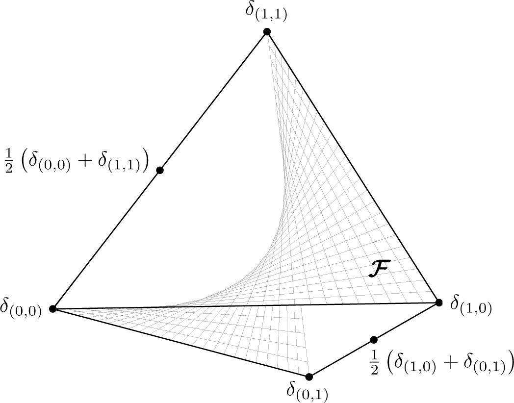
Example 1 (FACTORIZABLE DISTRIBUTIONS AND SPATIAL INTERDEPENDENCE). Let V be a finite set of units and Ωv, v ∊ V, corresponding state sets. Consider the tensorial map
with
The image
of this map, which consists of all factorizable and strictly positive probability distributions, is an exponential family in
with dim
. For the particular case of binary units, that is |Ωv| = 2 for all v, the dimension of F is equal to the number |V| of units. The following statement is well known [18]: The (−1)-projection of a distribution
on
is given by ⊗v∊V pv (the pv, v ∊ V, are the marginal distributions), and one has the representation
where H denotes the Shannon entropy [1]. As stated in the introduction, I(p) is a measure for the spatial interdependencies of the units. It vanishes exactly when the units are stochastically independent.
Before extending the spatial notion of interaction to a dynamical one, in Section 2.3 we consider the more general concept of separability of transition kernels.
2.3. Quantifying Non-Separability
2.3.1. Manifolds of Separable Transition Kernels
Consider a finite set V of units, corresponding state sets Ωv, v ∊ V, and two subsets A, B ⊂ V with B 6= ∅. A function
is called Markovian transition kernel if
for all ω ∊ ΩA, that is
The set of all such kernels is denoted by
. We write
for its interior and
respectively
as abbreviation in the case A = B. If A = ∅, then ΩA consists of exactly one element, namely the empty configuration ϵ. In that case,
can naturally be identified with
, ω ∊ ΩB.
Given a probability distribution
and a transition kernel
, the conditional entropy for (p, K) is defined as
For two random variables X, Y with Prob{X = ω} = p(ω) for all ω ∊ ΩA, and Prob{Y = ω′ | X = ω} = K(ω′ | ω) for all ω ∊ ΩA with p(ω) > 0 and all ω′ ∊ ΩB, we set H(Y | X) := H(p, K).
In the present paper, the set
is interpreted as a model for the dynamics of interacting units, and the information flow associated with this dynamics is studied in Section 2.4. In the present section, we introduce a general notion of separability of transition kernels in order to capture all examples that are discussed in the paper in a unified way.
Consider a family
where the Ai and Bi are subsets of V. We assume that {B1,…, Bn} is a partition of V, that is Bi ≠ ∅ for all i, Bi ∩ Bj = ∅ for all i ≠ j, and
. Now consider the corresponding tensorial map
with
The image
of
is a submanifold of
with
Its elements are the separable transition kernels with respect to
.
Here are the most important examples:
Examples and Definitions 1.
- If we set , the tensorial map is nothing but the identity , and therefore one has .
- Consider the case where no temporal information is transmitted but all spatial information: . In that case the tensorial map reduces to the natural embeddingwhich assigns to each probability distribution p the kernelTherefore, we write .
- In addition to the splitting in time which is described in example (2), consider also a complete splitting in space: . Then we recover the tensorial map of Example 1. Thus, can be identified with .
- To model the important class of parallel information processing, we set . Here, each unit “computes” its new state on the basis of all current states according to a kernel . The transition from a configuration ω = (ωv)v∊V of the whole system to a new configuration is done according to the following composed kernel in :
- In applications, parallel processing is adapted to a graph G = (V, E) – here, E ⊂ V × V denotes the set of edges – in order to model constraints for the information flow in the system. This is represented by . Each unit v is supposed to process only information from its parents pa(v) = {μ ∊ V: (μ, v) ∊ E}, which is modeled by a transition kernel . The parallel transition of the whole system is then described by
- Now, we introduce the example of parallel processing that plays the most important role in the present paper: Consider non-empty and pairwise distinct subsystems S1,…, Sn of V with V = S1⊎· · ·⊎Sn and define . It describes {S1,…, Sn}-split information processing, where the subsystems do not interact with each other. Each subsystem Si only processes information from its own current state according to a kernel . The composed transition of the whole system is then given byFor the completely split case, where the subsystems are the elementary units, we define .
2.3.2. Non-Separability as Divergence from Separability
Consider a Markov chain Xn = (Xv,n)v V, n = 0, 1, 2,…, that is given by an initial distribution
and a kernel
. The probabilistic properties of this stochastic process are determined by the following set of finite marginals:
Thus, the set of Markov chains on ΩV can be identified with
and we also use the notation {Xn} = {X0, X1, X2,…} instead of (p, K). The interior MC(ΩV ) of the set of Markov chains carries the natural dualistic structure from
, which is induced by the diffeomorphic composition map
,
(⊗ can be extended to a continuous surjective map
). Thus, we can talk about exponential families and (−1)-projections in MC(ΩV). The “distance” D((p, K) || (p′, K′)) from a Markov chain (p, K) to another one (p′, K′) is given by
with
For a set
, we introduce the exponential family (see Proposition 3)
which has dimension
.
The set of all these exponential families is partially ordered by inclusion with MC(ΩV) as the greatest element and MCfac(ΩV ) as the least one. This ordering is connected with the following partial ordering ≼ of the sets
: Given
and
, we write
(
coarser than
) iff for all (A, B) ∊ there exists a pair (A′, B′) ∊′ with A ⊂ A′ and B ⊂ B′. One has
Thus, coarsening enlarges the corresponding manifold (the proof is given in the appendix).
Now, we describe the (−1)-projections on the exponential families
:
Proposition 1. Let (p, K) be a Markov chain in MC(ΩV ) and S ≼S ′. Then:
- (PROJECTION) The (−1)-projection of (p, K) on is given by (p, ) with. Here, the kernels denote the corresponding marginals of K:is the projection of K on with respect to p.
- (ENTROPIC REPRESENTATION) The corresponding divergence is given by
- (PYTHAGORIAN THEOREM) One has
If
, that is K(ω′|ω) = p(ω), ω, ω′ ∊ ΩV, with a probability distribution
, then the divergence Dp(K||Kfac) is nothing but the measure I(p) for spatial interdependencies that has been discussed in the introduction and in Example 1. More generally, we interpret the divergence
as a natural measure for the non-separability of (p, K) with respect to
. The corresponding function
has a unique continuous extension to the set
of all Markov chains which is also denoted by
(see Lemma 4.2 in [55]). Thus, non-separability is defined for not necessarily strictly positive Markov chains.
2.4. Application to Stochastic Interaction
2.4.1. The Definition of Stochastic Interaction
As stated in the introduction we use the concept of complexity that is described by the formal definition in Equation (20) in order to define stochastic interaction.
Let V be a set of units and Ωv, v ∊ V, corresponding state sets. Furthermore, consider non-empty and pairwise distinct subsystems S1,…, Sn ⊂ V with V = S1 ⊎⋯⊎ Sn. The stochastic interaction of S1,…, Sn with respect to
is quantified by the divergence of (p, K) from the set of Markov chains that represent {S1,…, Sn}-split information processing, where the subsystems do not interact with each other (see Examples and Definitions 1 (6)). More precisely, we define the stochastic interaction (of the subsystems S1,…, Sn) to be the function
with
In the case of complete splitting of V = {v1,…, vn} into the elementary units, that is Si := {vi}, i = 1,…, n, we simply write I instead of I{v1},…,{vn}.
The definition of stochastic interaction given by Equation (25) is consistent with the complexity concept that is discussed in the introduction.
Here are some basic properties of I, which are well known in the spatial setting of Example 1:
Proposition 2. Let V be a set of units, Ωv, v ∊ V, corresponding state sets, and Xn = (Xv,n)v∊V, n = 0, 1, 2,…, a Markov chain on ΩV. For a subsystem S ⊂ V, we write XS,n := (Xv,n)v∊S. Assume that the chain is given by, where p is a stationary distribution with respect to K. Then the following holds:
- A, B ⊂ V, A, B ≠ ∅, A ∩ B = ∅, A ⊎ B = V ⇒
- If the process is parallel, then
- If the process is adapted to a graph (V, E) then
In the statements (iii) and (iv), the conditional mutual information MI(X; Y | Z) of two random variables X, Y with respect to a third one Z is defined to be the difference H(X | Z) − H(X | Y, Z) (see p. 22 in [58]).
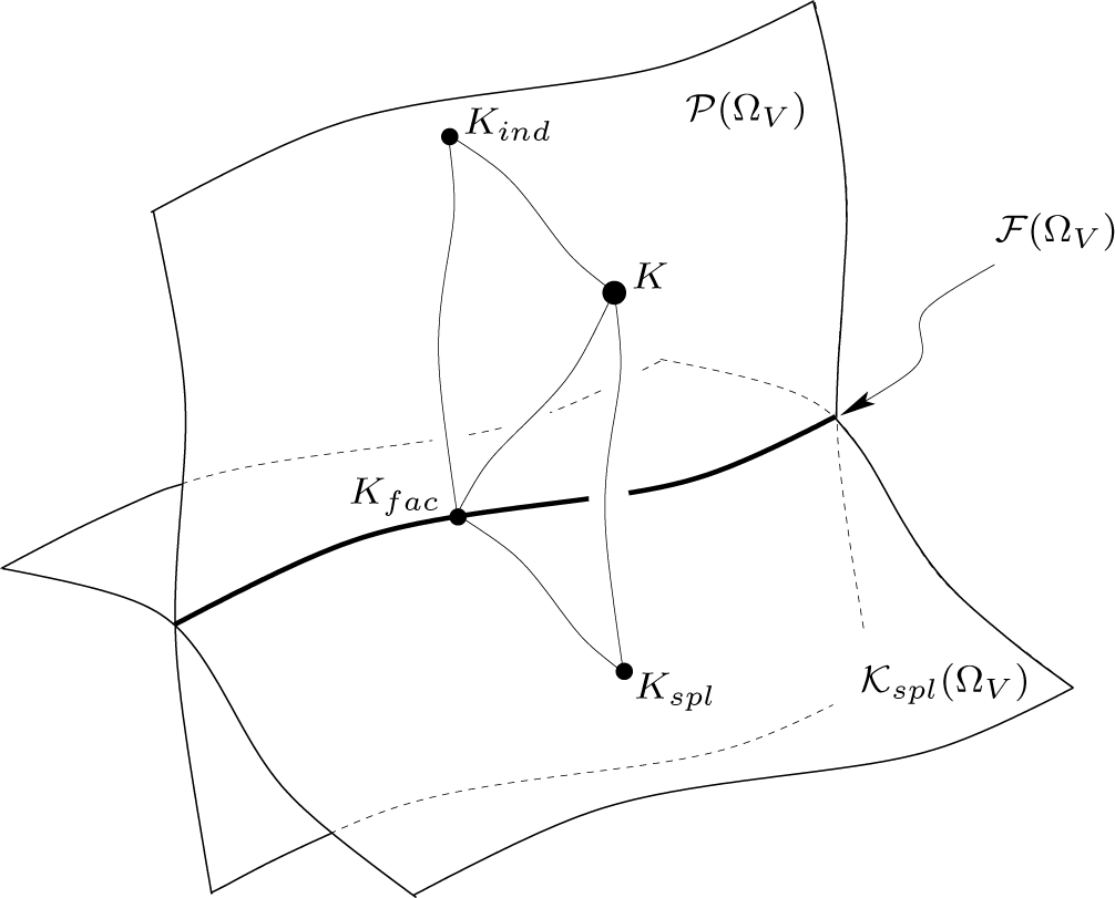
If Xn+1 and Xn are independent for all n, the stochastic interaction I{Xn} reduces to the measure I(p) for spatial interdependencies with respect to the stationary distribution p of {Xn} (see Example 1). Thus, the dynamical notion of stochastic interaction is a generalization of the spatial one. Geometrically, this can be illustrated as follows. In addition to the projection Kspl of the kernel K ∊ MC(ΩV) with respect to a distribution
on the set of split kernels, we consider its projections Kind and Kfac on the set
of independent kernels and on the subset
, respectively. From Proposition 1 we know
According to the Pythagorian relation (Proposition 1 (iii)), we get the following representation of stochastic interaction:
In the particular case of an independent process, the divergences Dp(K || Kind) and Dp(Kspl || Kfac) in Equation (29) vanish, and the stochastic interaction coincides with spatial interdependence.
2.4.2. Examples
Example 2 (SOURCE AND RECEIVER). Consider two units 1 = source and 2 = receiver with the state sets Ω1 and Ω2. Assume that the information flow is adapted to the graph G = {{1, 2}, {(1, 2)}}, which only allows a transmission from the first unit to the second. In each transition from time n to n + 1, a state X1,n+1 of the first unit is chosen independently from X1,n according to a probability distribution
. The state X2,n+1 of the second unit at time n + 1 is “computed” from X1,n according to a kernel
. Using formula Equation (28), we have
This is the well-known mutual information of the variables X2,n+1 and X1,n, which has a temporal interpretation within the present approach. It plays an important role in coding and information theory [58].
Example 3 (TWO BINARY UNITS I). Consider two units with the state sets {0, 1}. Each unit copies the state of the other unit with probability 1 − ε. The transition probabilities for the units are given by the following tables:

| K(1)(y′| (x, y)) | 0 | 1 |
|---|---|---|
| (0, 0) | 1−ε | ε |
| (0, 1) | ε | 1 −ε |
| (1, 0) | 1 −ε | ε |
| (1, 1) | ε | 1 − ε |
| K(2)(y′| (x, y)) | 0 | 1 |
|---|---|---|
| (0, 0) | 1−ε | ε |
| (0, 1) | 1 − ε | ε |
| (1, 0) | ε | 1 − ε |
| (1, 1) | ε | 1 − ε |
The transition kernel
for the corresponding parallel dynamics of the whole system is then given by
| K((x', y')|(x, y)) | (0, 0) | (0, 1) | (1, 0) | (1, 1) |
|---|---|---|---|---|
| (0, 0) | (1−ε)2 | (1−ε)ε | ε(1−ε) | ε2 |
| (0, 1) | ε(1−ε) | ε2 | (1−ε)2 | (1−ε)ε |
| (1, 0) | (1−ε)ε | (1−ε)2 | ε2 | ε(1−ε) |
| (1, 1) | ε2 | ε(1−ε) | (1−ε)ε | (1−ε)2 |
Note that for ε ∊ {0, 1}, K corresponds to the deterministic transformations
which in an intuitive sense describe complete information exchange of the units. With the unique stationary probability distribution p = (
,
,
,
) one can easily compute the marginal kernels
| K1(x′|x) | 0 | 1 |
|---|---|---|
| 0 | ||
| 1 |
| K2(y′|y) | 0 | 1 |
|---|---|---|
| 0 | ||
| 1 |
The shape of this function is shown in Figure 3.
This function is symmetric around
where it vanishes. In ε = 0 and ε = 1 it attains its maximal value 2 ln 2. As stated above, this corresponds to the deterministic transformations with complete information exchange.
Example 4 (TWO BINARY UNITS II). Consider again two binary units with the state sets {0, 1} and the transition probabilities
| K(1)(x′| (x, y)) | 0 | 1 |
|---|---|---|
| (0, 0) | 1 | 0 |
| (0, 1) | 1−ε | ε |
| (1, 0) | ε | 1−ε |
| (1, 1) | 0 | 1 |
| K(2)(y′| (x, y)) | 0 | 1 |
|---|---|---|
| (0, 0) | 0 | 1 |
| (0, 1) | 1−ε | ε |
| (1, 0) | ε | 1−ε |
| (1, 1) | 1 | 0 |
The transition kernel
of the corresponding parallel dynamics is given by
| K((x', y')|(x, y)) | (0, 0) | (0, 1) | (1, 0) | (1, 1) |
|---|---|---|---|---|
| (0, 0) | 0 | 1 | 0 | 0 |
| (0, 1) | (1−ε)2 | (1−ε)ε | ε(1−ε) | ε2 |
| (1, 0) | ε2 | ε(1−ε) | (1−ε)ε | (1−ε)2 |
| (1, 1) | 0 | 0 | 1 | 0 |
Note that for ε ∊ {0, 1}, K corresponds to the deterministic transformations
Thus in an intuitive sense, for ε = 1 the units completely interact with each other, and for ε = 0 there is no interaction. For ε ∊]0, 1[ we compute the interaction with respect to the unique stationary probability distribution
With the corresponding marginal kernels
| K1(x′|x) | 0 | 1 |
|---|---|---|
| 0 | ||
| 1 |
| K2(y′|y) | 0 | 1 |
|---|---|---|
| 0 | ||
| 1 |
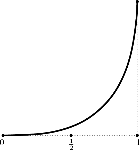
and Equation (27), we get
This function is monotonically increasing from the minimal value 0 (no interaction) in ε = 0 to its maximal value 2 ln 2 (complete interaction) in ε = 1.
3. Conclusions
Following the general concept that complexity is characterized by the divergence of a composed system from the superposition of its elementary parts, information geometry has been used to derive a measure for spatio-temporal interdependencies among a finite set of units, which is referred to as stochastic interaction. This generalizes the well-known measure for spatial interdependence that is quantified by the Kullback-Leibler divergence of a probability distribution from its factorization [18,55]. Thereby, previous work by Ay [23] is continued, where the optimization of dependencies among stochastic units has been proposed as a principle for neural organization in feed-forward networks. Of course, the present setting is much more general and provides a way to consider also recurrent networks. The dynamical properties of strongly interacting units in the sense of the present paper are studied by Ay and Wennekers in [24], where the emergence of determinism and structure in such systems is demonstrated.
Conflicts of Interest
The author declares no conflict of interest.
Appendix
Appendix: Proofs
Proposition 3. The manifold is an exponential family in MC(ΩV ).
Proof. To see this, consider the functions ΩV × ΩV → ℝ
and
It is easy to verify that the image of
under the map ⊗ is the following exponential family in
:
Here, Θ denotes the normalization factor, which depends on the λ-parameters. In particular, each element in
can be expressed in the following way
Proof of Implication (24). If
then there exists a partition Mi, i = 1,…, n, of the index set {1,…, m} such that
Let (p, K) be a Markov chain in
. Then there exist
with
The kernels
are contained in
, and therefore we get
.
Proof of Proposition 1.
- Consider the following strictly convex function ( denotes the set of positive real numbers)Here, λ and the are Lagrangian parameters. Note that in the case and , the value F (x, y) is nothing but the divergence of (p, K) from (x, (y)). In order to get the Markov chain that minimizes the divergence we have to compute the partial derivatives of F:andFor a critical point (x, y), the partial derivatives vanish. We get the following solution:andFrom Theorem 3.10 in [17] we know that this solution is the (−1)-projection of (p, K) onto . It is given by the initial distribution p and the corresponding marginals , of K.
- With (i) we get
- According to Equation (24) we have MCS (ΩV ) ⊆ MCS0 (ΩV ), and the statement follows from the Pythagorian theorem ([17], p. 62, Theorem 3.8).
Proof of Proposition 2.
- This follows from Proposition 1 (ii).
- We apply (i):
- For parallel processing, one hasThe statement is then implied by (i).
- This follows from (iii) and the Markov property for (V, E)-adapted Markov chains.
References
- Shannon, C.E. A mathematical theory of communication. Bell Syst. Tech. J. 1948, 27, 379–423. [Google Scholar]
- Attneave, F. Informational aspects of visual perception. Psychol. Rev. 1954, 61, 183–193. [Google Scholar]
- Barlow, H.B. Possible principles underlying the transformation of sensory messages. Sens. Commun. 1961, 217–234. [Google Scholar]
- Laughlin, S. A simple coding procedure enhances a neuron’s information capacity. Z. Naturforsch. 1981, 36, 910–912. [Google Scholar]
- Linsker, R. Self-organization in a perceptual network. Computer 1988, 21, 105–117. [Google Scholar]
- Hubel, D.H.; Wiesel, T.N. Functional Architecture of Macaque Monkey Visual Cortex (Ferrier lecture). Proc. R. Soc. Lond. B 1977, 198, 1–59. [Google Scholar]
- Hubel, D.H.; Wiesel, T.N. Brain Mechanisms of Vision. Sci. Am. 1979, 241, 150–162. [Google Scholar]
- Bell, A.J.; Sejnowski, T.J. An information-maximization approach to blind separation and blind deconvolution. Neural Comput. 1995, 7, 1129–1159. [Google Scholar]
- Tononi, G.; Sporns, O.; Edelmann, G.M. A measure for brain complexity: Relating functional segregation and integration in the nervous system. Proc. Natl. Acad. Sci. USA 1994, 91, 5033–5037. [Google Scholar]
- Tononi, G.; Sporns, O. Measuring information integration. BMC Neurosci. 2003, 4. [Google Scholar] [CrossRef] [Green Version]
- Tononi, G. An information integration theory of consciousness. BMC Neurosci. 2004, 5. [Google Scholar] [CrossRef] [Green Version]
- Balduzzi, D.; Tononi, G. Integrated Information in Discrete Dynamical Systems: Motivation and Theoretical Framework. PLoS Comp. Biol. 2008, 4, 1000091. [Google Scholar]
- Tononi, G. Consciousness as Integrated Information: A Provisional Manifesto. Biol. Bull. 2008, 215, 216–242. [Google Scholar]
- Barrett, A.B.; Seth, A.K. Practical Measures of Integrated Information for Time-Series Data. PLoS Comp. Biol. 2011, 7, 1001052. [Google Scholar]
- Edlund, J.; Chaumont, N.; Hintze, A.; Koch, C.; Tononi, G.; Adami, C. Integrated Information Increases with Fitness in the Evolution of Animats. PLoS Comp. Biol. 2011, 7, e1002236. [Google Scholar]
- Ay, N. Information Geometry on Complexity and Stochastic Interaction. MPI MiS Preprint, 95/2001. Available online: http://www.mis.mpg.de/publications/preprints/2001/prepr2001-95.html accessed on 7 December 2001.
- Amari, S.I.; Nagaoka, H. Methods of Information Geometry; Translations of Mathematical Monographs; AMS and Oxford University Press: New York, NY, USA, 2000. [Google Scholar]
- Amari, S.I. Information Geometry on Hierarchy of Probability Distributions. IEEE Trans. Inf. Theory 2001, 47, 1701–1711. [Google Scholar]
- McGill, W.J. Multivariate information transmission. Psychometrika 1954, 19, 97–116. [Google Scholar]
- Kolchinsky, A.; Rocha, L.M. Prediction and Modularity in Dynamical Systems, Advances in Artificial Life, Proceedings of the Eleventh European Conference on the Syntheses and Simulation of Living Systems (ECAL 2011); MIT Press: Paris, France, 2011; pp. 423–430.
- Arsiwalla, X.D.; Verschure, P.F.M.J. Integrated Information for Large Complex Networks, Proceedings of 2013 International Joint Conference on Neural Networks (IJCNN), Dallas, TX, USA, 4–9 August 2013; pp. 620–626.
- Amari, S.I. Natural gradient works efficiently in learning. Neural Comput. 1998, 10, 251–276. [Google Scholar]
- Ay, N. Locality of global stochastic interaction in directed acyclic networks. Neural Comput. 2002, 14, 2959–2980. [Google Scholar]
- Ay, N.; Wennekers, T. Dynamical Properties of Strongly Interacting Markov Chains. Neural Netw. 2003, 16, 1483–1497. [Google Scholar]
- Wennekers, T.; Ay, N. Finite state automata resulting from temporal information maximization and a temporal learning rule. Neural Comput. 2005, 17, 2258–2290. [Google Scholar]
- Ay, N.; Montúfar, G.; Rauh, J. Selection Criteria for Neuromanifolds of Stochastic Dynamics, Advances in Cognitive Neurodynamics (III), Proceedings of the Third International Conference on Cognitive Neurodynamics 2011, Hokkaido, Japan, 9–13 June 2011; pp. 147–154.
- Ay, N. Geometric Design Principles for Brains of Embodied Agents; Santa Fe Institute Working Paper 15-02-005; Santa Fe Institute: Santa Fe, NM, USA, 2015. [Google Scholar]
- Wennekers, T.; Ay, N. Temporal infomax leads to almost deterministic dynamical systems. Neurocomputing 2003, 52-4, 461–466. [Google Scholar]
- Wennekers, T.; Ay, N. Temporal Infomax on Markov chains with input leads to finite state automata. Neurocomputing 2003, 52-4, 431–436. [Google Scholar]
- Wennekers, T.; Ay, N. Spatial and temporal stochastic interaction in neuronal assemblies. Theory Biosci 2003, 122, 5–18. [Google Scholar]
- Wennekers, T.; Ay, N. Stochastic interaction in associative nets. Neurocomputing 2005, 65, 387–392. [Google Scholar]
- Wennekers, T.; Ay, N. A temporal learning rule in recurrent systems supports high spatio-temporal stochastic interactions. Neurocomputing 2006, 69, 1199–1202. [Google Scholar]
- Wennekers, T.; Ay, N.; Andras, P. High-resolution multiple-unit EEG in cat auditory cortex reveals large spatio-temporal stochastic interactions. Biosystems 2007, 89, 190–197. [Google Scholar]
- Schreiber, T. Measuring information transfer. Phys. Rev. Lett. 2000, 85, 461–464. [Google Scholar]
- Ay, N.; Polani, D. Information Flows in Causal Networks. Adv. Complex Syst. 2008, 11, 17–41. [Google Scholar]
- Ay, N.; Krakauer, D.C. Geometric robustness theory and biological networks. Theory Biosci. 2007, 2, 93–121. [Google Scholar]
- Ay, N. A Refinement of the Common Cause Principle. Discret. Appl. Math. 2009, 157, 2439–2457. [Google Scholar]
- Steudel, B.; Ay, N. Information-theoretic inference of common ancestors. Entropy 2015, 17, 2304–2327. [Google Scholar]
- Moritz, P.; Reichardt, J.; Ay, N. Discriminating between causal structures in Bayesian Networks via partial observations. Kybernetika 2014, 50, 284–295. [Google Scholar]
- Pearl, J. Causality: Models, Reasoning and Inference; Cambridge University Press: Cambridge, UK, 2000. [Google Scholar]
- Janzing, D.; Balduzzi, D.; Grosse-Wentrup, M.; Schölkopf, B. Quantifying causal influences. Ann. Stat. 2013, 41, 2324–2358. [Google Scholar]
- Ay, N.; Knauf, A. Maximizing Multi-Information. Kybernetika 2007, 42, 517–538. [Google Scholar]
- Ay, N.; Olbrich, E.; Bertschinger, N.; Jost, J. A Geometric Approach to Complexity. Chaos 2011, 21, 037103. [Google Scholar]
- Ay, N.; Olbrich, E.; Bertschinger, N.; Jost, J. A Unifying Framework for Complexity Measures of Finite Systems, Proceedings of the European Conference on Complex Systems 2006 (ECCS’06), Oxford University, Oxford, UK, 25–29 September 2006; p. 80.
- Adami, C. The Use of Information Theory in Evolutionary Biology. Ann. NY Acad. Sci. 2012, 1256, 49–65. [Google Scholar]
- Ay, N.; Bertschinger, N.; Der, R.; Guettler, F.; Olbrich, E. Predictive information and explorative behavior of autonomous robots. Eur. Phys. J. B 2008, 63, 329–339. [Google Scholar]
- Zahedi, K.; Ay, N.; Der, R. Higher coordination with less control—A result of information maximisation in the sensorimotor loop. Adapt. Behav. 2010, 18, 338–355. [Google Scholar]
- Ay, N.; Bernigau, H.; Der, R.; Prokopenko, M. Information driven self-organization: The dynamical system approach to autonomous robot behavior. Theory Biosci 2011. [Google Scholar] [CrossRef]
- Kahle, T.; Olbrich, E.; Jost, J.; Ay, N. Complexity Measures from Interaction Structures. Phys. Rev. E 2009, 79, 026201. [Google Scholar]
- Olbrich, E.; Bertschinger, N.; Ay, N.; Jost, J. How should complexity scale with system size? Eur. Phys. J. B 2008, 63, 407–415. [Google Scholar]
- Amari, S.I. Differential-Geometric Methods in Statistics (Lecture Notes in Statistics); Springer: Berlin, Germany, 1985. [Google Scholar]
- Kullback, S.; Leibler, R.A. On information and sufficiency. Ann. Math. Stat. 1951, 22, 79–86. [Google Scholar]
- Csiszár, I. I-divergence geometry of probability distributions and minimization problems. Ann. Probab. 1975, 3, 146–158. [Google Scholar]
- Csiszár, I. On topological properties of f-divergence. Stud. Sci. Math. Hungar. 1967, 2, 329–339. [Google Scholar]
- Ay, N. An Information-Geometric Approach to a Theory of Pragmatic Structuring. Ann. Probab. 2002, 30, 416–436. [Google Scholar]
- Rao, C.R. Information and the accuracy attainable in the estimation of statistical parameters. Bull. Calcutta Math. Soc. 1945, 37, 81–91. [Google Scholar]
- Hofbauer, J.; Sigmund, K. Evolutionary Games and Population Dynamics; Cambridge University Press: Cambridge, UK, 1998. [Google Scholar]
- Cover, T.M.; Thomas, J.A. Elements of Information Theory; Wiley Series in Telecommunications; Wiley-Interscience: New York, NY, USA, 1991. [Google Scholar]
Figure 1.
F denotes the set of factorizable distributions on {0, 1} × {0, 1}.

Figure 2.
Illustration of the two ways of projecting K onto
. Corresponding application of the Pythagorean theorem leads to Equation (29).
Figure 2.
Illustration of the two ways of projecting K onto
. Corresponding application of the Pythagorean theorem leads to Equation (29).

Figure 3.
Illustration of the stochastic interaction I{Xn} as a function of ε. For the extreme values of ε we have maximal stochastic interaction, which corresponds to a complete information exchange in terms of (x, y) ↦ (y, x) for ε = 0 and (x, y) ↦ (1 − y, 1 − x) for ε = 1. For
, the dynamics is maximally random, which is associated with no interaction of the nodes.
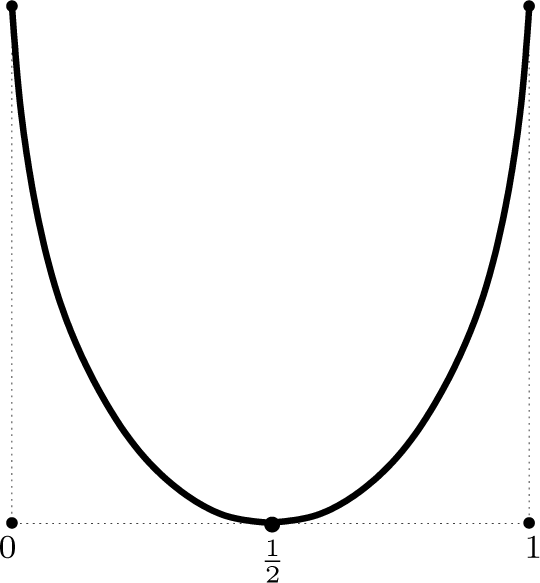
Figure 4.
Illustration of the stochastic interaction I{Xn} as a function of ε. For ε = 0, the two units update their states with no information exchange: (x, y) ↦ (x, 1 − y). For ε = 1, there is maximal information exchange in terms of (x, y) ↦(y, 1 − x).
Figure 4.
Illustration of the stochastic interaction I{Xn} as a function of ε. For ε = 0, the two units update their states with no information exchange: (x, y) ↦ (x, 1 − y). For ε = 1, there is maximal information exchange in terms of (x, y) ↦(y, 1 − x).
© 2015 by the authors; licensee MDPI, Basel, Switzerland This article is an open access article distributed under the terms and conditions of the Creative Commons Attribution license (http://creativecommons.org/licenses/by/3.0/).
Share and Cite
MDPI and ACS Style
Ay, N. Information Geometry on Complexity and Stochastic Interaction. Entropy 2015, 17, 2432-2458. https://doi.org/10.3390/e17042432
AMA Style
Ay N. Information Geometry on Complexity and Stochastic Interaction. Entropy. 2015; 17(4):2432-2458. https://doi.org/10.3390/e17042432
Chicago/Turabian StyleAy, Nihat. 2015. "Information Geometry on Complexity and Stochastic Interaction" Entropy 17, no. 4: 2432-2458. https://doi.org/10.3390/e17042432