Entropic-Skins Geometry to Describe Wall Turbulence Intermittency

Abstract

In order to describe the phenomenon of intermittency in wall turbulence and, more particularly, the behaviour of moments $⟨{\left|\delta V\right|}_r{}^p⟩$ and $⟨{\mathrm{\epsilon }}_r{}^p⟩$and intermittency exponents ζ_P with the order p and distance to the wall, we developed a new geometrical framework called “entropic-skins geometry” based on the notion of scale-entropy which is here applied to an experimental database of boundary layer flows. Each moment has its own spatial multi-scale support Ω_p (“skin”). The model assumes the existence of a hierarchy of multi-scale sets Ω_p ranged from the “bulk” to the “crest”. The crest noted characterizes the geometrical support where the most intermittent (the highest) fluctuations in energy dissipation occur; the bulk is the geometrical support for the whole range of fluctuations. The model assumes then the existence of a dynamical flux through the hierarchy of skins. The specific case where skins display a fractal structure is investigated. Bulk fractal dimension ${\mathrm{\Delta }}_f$ and crest dimension ${\mathrm{\Delta }}_{\infty }$ are linked by a scale-entropy flux defining a reversibility efficiency $\gamma =({\mathrm{\Delta }}_f-{\mathrm{\Delta }}_{\infty })/(d-{\mathrm{\Delta }}_{\infty })$ (d is the embedding dimension). The model, initially developed for homogeneous and isotropic turbulent flows, is applied here to wall bounded turbulence where intermittency exponents are measured by extended self-similarity. We obtained for intermittency exponents the analytical expression ${\zeta }_p=\left[({\mathrm{\Delta }}_{\infty }(1-\gamma )+3\gamma -2)/3\right]p+(3-{\mathrm{\Delta }}_{\infty })(1-{\gamma }^{p/3})$with γ ≈ 0.36 in agreement with experimental results.

1. Introduction: Intermittency in Wall and Bounded Turbulence

1.1. Intermittency in Turbulence: Departures to Kolmogorov’s Theory

Kolmogorov’s theory of fully developed turbulence assumes that energy dissipation occurs through an homogenous and isotropic way [1,2]. Following Kolmogorov’s formalism, turbulent flows are usually studied using structure functions $\langle {\left|\delta V\right|}_r{}^p\rangle$ or $\langle {\mathrm{\epsilon }}_r{}^p\rangle$ where ${\left|\delta V\right|}_r$ is the velocity difference across a distance r and ε_r, the rate of energy dissipation per unit mass averaged over a ball of size r. Kolmogorov’s classical theory, which postulates an homogeneous energy dissipation (that should be space-filling), predicts universal scaling laws $\langle {\left|\delta V\right|}_r{}^p\rangle \sim r^{{\zeta }_p}$ and $\langle {\mathrm{\epsilon }}_r{}^p\rangle ~r^{{\tau }_p}$ for high Reynolds numbers and scales belonging to the inertial range ( $\eta \ll r\ll r_0$ where η and r₀ are respectively the Kolmogorov’s scale and the integral scale). The scaling exponents ζ_P and τ_p are linked through ζ_P = τ_p/3 + p/3 due to the refined similarity hypothesis: $\langle {\left|\delta V\right|}_r{}^p\rangle =\langle {\mathrm{\epsilon }}_r{}^{p/3}\rangle r^{p/3}$ [3]. For these conditions, Kolmogorov predicted that the exponents ζ_P should follow a linear law: ζ_P = p/3, i.e., τ_p/3 = 0. The case p = 2 (ζ₂ = 2/3) corresponds to the Kolmogorov's spectrum: $E(k)=C_K{\mathrm{\epsilon }}^{2/3}{k}^{-5/3}$, where ε represents the rate of energy dissipation assumed to be a scale-independent quantity. Experimental and numerical studies showed a clear deviation of the exponents ζ_P from this linear value predicted in the context of Kolmogorov’s assumptions; the departure is weak for small values of p; for p = 2, the implication on the spectrum is weak (ζ₂ ≈ 0.70 instead of 2/3: the slope of spectrum is 1 + ζ₂) but this departure increases when p increases. For the sake of clearness, the exponents corresponding to this specific case of a homogeneous and isotropic turbulent flow will be noted ζ_p^HI. Several models have been proposed to describe this behaviour; the log-normal model [4], the β-model [5,6] and, more recently, the She–Levêque model [7] which displays a remarkable agreement with the experimental data. In this paper, we will use the property of extended self-similarity [8] to determine intermittency exponents.

1.2. Extended Self-Similarity and Intermittency Exponents for Homogenous Isotropic Turbulence

It has been observed that the existence of the scaling laws $\langle {\left|\delta V\right|}_r{}^p\rangle \sim r^{{\zeta }_p}$, expected for high Reynolds numbers, is difficult to evidence for moderate Reynolds numbers since the pertinent scale range is small which makes the determination of scaling exponents difficult. To overcome this experimental limitation, Benzi et al. [8] introduced extended self-similarity (hereafter ESS). The authors showed that each structure function $\langle {\left|\delta V\right|}_r{}^p\rangle$, even if it does not follow a power law with scale, is a power law of the particular structure function $\langle {\left|\delta V\right|}_r{}^3\rangle$. The remarkable point here is that the exponent corresponding to this power law (different from p/3, otherwise it would be not intermittent) can be identified to the ratio ζ_p/ζ₃ of the scaling exponents ζ_p that would be ideally obtained for high Reynolds numbers. Using the exact result ζ₃ = 1 [2], the absolute exponents ζ_p can then be determined. Some studies showed that the universal quantities in a turbulent flow were in fact the relative scaling exponents ζ_p/ζ₃ and not the absolute ones [9]. ESS thus represents an indirect determination of scaling exponents via measurements obtained at low and moderate Reynolds numbers in order to gather results that would constitute the limit at high Reynolds numbers. It has been shown that ESS result implies, more generally, that every structure function $\langle {\left|\delta V\right|}_r{}^p\rangle$ is a power-law function of any other structure function $\langle {\left|\delta V\right|}_r{}^q\rangle$ whose exponent corresponds to ζ_p/ζ_q.

For homogeneous and isotropic turbulent flows (scaling exponents noted ζ_p^HI), intermittency represents for low orders a slight deviation from the Kolmogorov’s theory; its effect on the spectrum of turbulence (order 2) is almost negligible but departure is important at large orders. The values now widely accepted are the following [6,8]: ζ₁^HI = 0.36, ζ₂^HI = 0.70, ζ₃^HI = 1, ζ₄^HI = 1.28, ζ₅^HI = 1.53, ζ₆^HI = 1.77, ζ₇^HI = 2.01 and ζ₈^HI = 2.23.

1.3. Intermittency for Wall and Bounded Turbulence

The fact that ESS argued that the universal quantities to consider are not the absolute scaling exponents ζ_p but the relative ones, ζ_p/ζ₃ generates a new interest for inhomogenous flows in order to understand the structure of turbulence and intermittency. A new kind of study linked to what can be called “bounded turbulent flows” emerged around 20 years ago. Protas et al. [10] studied a simulated two-dimensional turbulence in wakes behind bluff bodies corresponding to a homogeneous and isotropic turbulent flow. They showed that scaling exponents determined by ESS vary with distance to the obstacle and that intermittency visualized by the deviation of ζ_p relatively to linear Kolmogorov’s law p/3 increases towards the wall. Far from the obstacle, the values associated with homogeneous and isotropic turbulence are recovered. The experimental study conducted by Gaudin et al. [11] in turbulent wake flows led to the same qualitative result showing a continuous transition between a “bounded turbulence” near the cylinder and a homogeneous and isotropic turbulence downstream. Onorato et al. [12] evidenced experimentally in the case of a turbulent channel flow that the “region in which the small scale intermittency is stronger corresponds to the buffer layer” and, more exactly, to the range $10\le y^{+}\le 40$. At the value y⁺ = 310, the values ζ_p^HI corresponding to homogeneous and isotropic turbulence are recovered. Toschi et al. [13] also observed (numerically) in a turbulent channel flow a “growth of intermittency towards the boundaries”; they evidenced two characteristic zones: the first (y⁺ ≥ 100) is called “homogeneous” because it displays the scaling exponents ζ_p^HI found in homogeneous and isotropic turbulence; the second one (20 ≤ y⁺ ≤ 50), much more intermittent, displays a larger deviation of ζ_p exponents relatively to the homogeneous case.

2. Multi-Scale Geometry of Turbulence and Intermittency: Entropic-Skins Model

2.1. Geometrical Features of Intermittency in Turbulence

Due to the progress of visualisation techniques provided namely by laser technology, fully developed turbulence can also be studied geometrically through the analysis of turbulent interfaces and turbulent fields of velocity obtained by Particle Image Velocimetry. In the wake of the development of fractal geometry, it has been proposed that turbulent interfaces could be fractal for scales belonging to the inertial scale range. The fractal dimension ${\mathrm{\Delta }}_f\approx 2.36$ emerged from many studies concerning clouds, turbulent jets, mixing or boundary layers [14]. This generality has led Sreeenivasan et al. [15] to affirm: “the apparent generality of this result must have a simple and basic explanation.” Vassilicos and Hunt [16] qualified this dimension as a “magic number”. The last decade showed that the multi-scale structure of turbulent interfaces is indeed much more complicated than simple scale invariance. Let us quote the work by Dimotakis and his collaborators who showed that fractal dimension has a scale-dependent character [17] as well as several studies in the field of turbulent combustion showing that pure fractal behaviour can only be a limit [18,19]. After these precisions, we should indicate that the scale-dependency of fractal dimensions or scaling exponents are not the central point of this study. We will assume in this paper that a scale-range large enough exists as far as a constant fractal dimension can be defined. We are mainly interested by the behaviour of the exponents ζ_p measured by ESS when the wall distance varies.

Another important observation in terms of geometrical features related to the fact that a turbulent flow displays a hierarchy of different structures when submitted to a specific thresholding. The quantity used for thresholding can be vorticity or the fluctuation of energy dissipation relatively to its mean; it has been shown that, for high Reynolds numbers, the highest fluctuations relative to the mean occur on a filamentary support (whose fractal dimension is Δ_∞ = 1) [20,21]. This leads to the idea that turbulence, at high Reynolds numbers, should now be described as a mixture of disordered structures characterized by low intensity fluctuations (the background) and ordered structures (filaments) where the highest fluctuations relative to the mean take place.

Since a fractal dimension exists for the flow in the cases where the threshold intensity chosen for energy dissipation or vorticity is low (with probably a link with Δ_f ≈ 2.36) and another fractal dimension exists for the highest values of the threshold leading to filaments (Δ_∞ = 1) and, furthermore, given the fact that if this threshold is null then fractal dimension is obviously the embedding dimension (d = 3 for a three-dimensional turbulence which is the case considered here), this implies that a hierarchy of fractal dimensions between d = 3 and Δ_∞ = 1 depending on the threshold must be introduced.

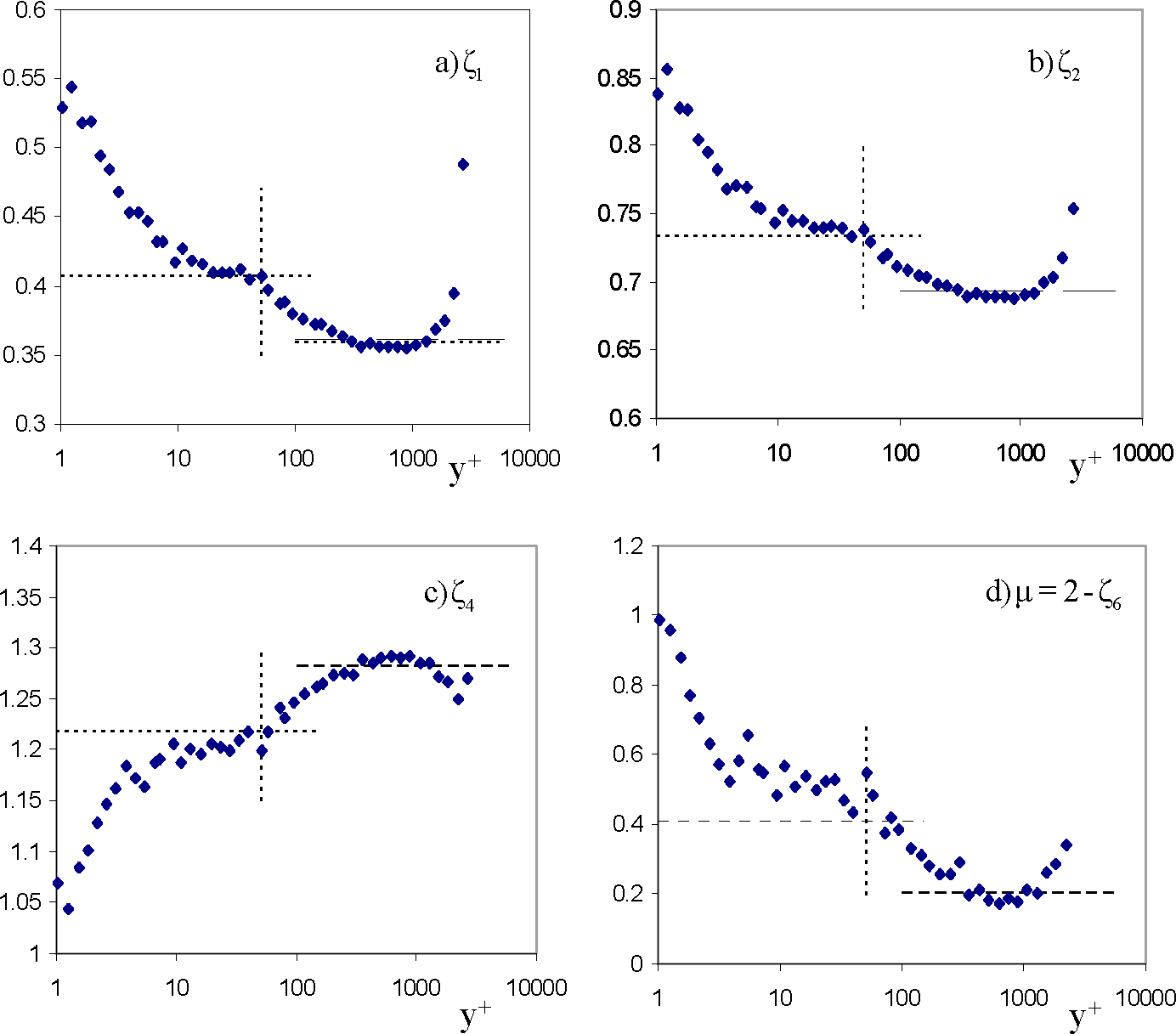
2.2. Wall Turbulence Intermittency through Structure Functions and Scaling Exponents

In order to explain the deviation from the Kolmogorov’s linear behaviour (ζ_p = p/3) associated with the phenomenon of intermittency, entropic-skins model (hereafter ESG) was proposed a few years ago [22,23]. It lies on the assumption that energy dissipation displays a range of fluctuations relative to its mean value and that these fluctuations, depending on their level, are characterized by a spatial support (the “active zone”) which is more or less extended. It then assumes that the value of a structure function is given by its active part: this means that there are zones of the fluid which do not contribute to the structure function. If f_p(r) is the volume fraction of the active part, we have $\langle {\mathrm{\epsilon }}_r{}^p\rangle =\overline{{\mathrm{\epsilon }}_r{}^p}{f}_p(r)$ where $\overline{{\mathrm{\epsilon }}_r{}^p}$ corresponds to the contribution due to the active part. Moreover, entropic-skins model assumes that this active part corresponding to the structure function $\langle {\mathrm{\epsilon }}_r{}^p\rangle$ is a fractal structure whose fractal dimension is ${\mathrm{\Delta }}_p$, depending on the order of the structure function. We interpret the order p as a parameter linked to a threshold on energy dissipation with two extrema: if p→0, Δ₀ = d = 3; if p→∞, Δ_∞ = 1. We associate the simple mean value (p = 1) to the classical fractal dimension Δ₁ = D_f. The whole range of fluctuations is thus investigated by varying p from 0 to p→∞. Usually p is taken as an integer but we emphasize that the order p can take any positive value and, namely, fractional values. We thus have $\langle {\mathrm{\epsilon }}_r{}^p\rangle =\overline{{\mathrm{\epsilon }}_r{}^p}{(r/r_0)}^{d-{\mathrm{\Delta }}_p}$. Moreover, we consider that the intermittency character is mainly provided by the fact that the active part which is characterized by the volume fraction is not space-filling. We therefore assume that the active part itself has a non-intermittent character: this implies that $\overline{{\mathrm{\epsilon }}_r{}^p}={\overline{{\mathrm{\epsilon }}_r}}^p$. This finally gives

$$\langle {\mathrm{\epsilon }}_r{}^p\rangle ={\overline{{\mathrm{\epsilon }}_r}}^p{(r/r_0)}^{d-{\mathrm{\Delta }}_p}$$

(1)

The case p = 1 gives $\langle {\mathrm{\epsilon }}_r\rangle =\overline{{\mathrm{\epsilon }}_r}{(r/r_0)}^{d-{\mathrm{\Delta }}_f}$. The quantity $\overline{{\mathrm{\epsilon }}_r}$ represents the mean energy dissipation of the active volume of the field at scale r while the quantity <ε_r> is the mean on the whole field: we have <ε_r> ≤ $\overline{{\mathrm{\epsilon }}_r}$ since f(r) ≤ 1. If U’ is the turbulent intensity of the flow, the total kinetic energy associated with a ball of size the integral scale r₀ is E_c = ρr₀^dU’². The characteristic time at integral scale being t₀ = r₀/U’, it implies that the power injected is P = E_c/t₀ = ρr₀^dU’³/r₀. This is an average for the entire field so we can write <ε_r> = P. It leads to $\overline{{\mathrm{\epsilon }}_r}=(U{\prime }^3/r_0){(r/r{}_0)}^{{\mathrm{\Delta }}_f-d}$. It is interesting to note that, if we define $m(r)=\rho r_0{}^d{(r/r_0)}^{d-{\mathrm{\Delta }}_f}$ as the active mass at scale r, then $\overline{{\mathrm{\epsilon }}_r}=P/m(r)$ is the mean energy dissipation of active part and corresponds to the power injected by unit of active mass. This implies that the quantity $\overline{{\mathrm{\epsilon }}_r}$ follows a power law with scale: $\overline{{\mathrm{\epsilon }}_r}\sim r^{\chi }$ with χ = Δ_f − d.

2.3. Entropic-Skins Model

To express structure functions as $\langle {\mathrm{\epsilon }}_r{}^p\rangle =\overline{{\mathrm{\epsilon }}_r{}^p}{f}_p(r)$, we need the spatial-extension of the set Ω_p which is defined by its volume fraction at scale r, f_p(r) = V_p(r)/V₀, where V_p(r) is the volume occupied by Ω_p at scale r in a total volume corresponding to integral scale V₀ = r₀^d. In mathematical terms, the set V_p(r) is equal to the volume of the “Minkowski sausage” of scale r of Ω_p set. If N_p(r) is the minimum number of balls of size needed to cover the set Ω_p, the volume is simply given by V_p(r) = N_p(r)r^d. We then introduce W_p(r) = 1/f_p(r) as the number of sets Ω_p necessary to fill the space and we define scale-entropy [19] by:

$$S_p\left(r\right)=ln\left[W_p\left(r\right)\right]with{W}_p\left(r\right)=V_0/V_p\left(r\right).$$

(2)

Scale-entropy can be defined even if the multi-scale set is not fractal since its volume fraction f_p(r) can always be defined. For the specific case where the set Ω_p being fractal, we have $V_p(r)={(r/r_0)}^{-{\mathrm{\Delta }}_p}{r}^d$; scale-entropy can then be easily written S_p(r) = (d − Δ_p)ln(r/r₀) in the fractal case. Let us come back to the general case without any assumption of fractality. We will use scale-entropy in order to define a dynamics in the hierarchy of the sets Ω_p between the two extrema Ω₀ and Ω_∞. To do so, we now consider two consecutive values of the order: p and p + dp where dp is a positive increment. This means that the range of fluctuations expressed by p varying from 0 to p→∞ is divided into an infinite number of layers having a thickness dp. The set Ω_p thus characterizes a layer (“skin”) of fluctuations in [p − dp/2; p + dp/2]; dp represents thus a sort of “thickness” for the set Ω_p in the order space. However, for the sake of clearness, we present here the case for dp = 1. The corresponding sets Ω_p and Ω_{p + 1} have a different scale entropy. The absolute value of scale-entropy is increasing from Ω_p to Ω_p+1, since fractal dimension is decreasing. We then define the scale-entropy jump at scale r between them by:

$$\delta S_p\left(r\right)=S_p\left(r\right)-S_{p-1}\left(r\right).$$

(3)

We interpret the quantity $\delta S_p^{\mathrm{in}}(r)=S_p^{}(r)-S_{p-1}^{}(r)$ as an input of scale-entropy for the set Ω_p coming from the lower hierarchical sets. The scale-entropy jump $\delta S_p^{\mathrm{out}}(r)=S_{p+1}^{}(r)-S_p^{}(r)$ is interpreted as an output for the set Ω_p which is expected to the higher hierarchical sets. We can define a quantity expressing how scale-entropy is transmitted through the set Ω_p via the transition from Ω_{p − 1} to Ω_{p + 1}

$${\gamma }_p(r)=\frac{\delta S_p^{\mathrm{out}}(r)}{\delta S_p^{\mathrm{in}}(r)}=\frac{S_{p+1}(r)-S_p(r)}{S_p(r)-S_{p-1}(r)}.$$

(4)

The quantity γ_p(r) is called the reversibility efficiency and characterizes the transition (referred to Ω_p) in terms of scale-entropy from Ω_{p − 1} to Ω_{p + 1}. If γ_p(r) = 1, the phenomenon is non-intermittent and there is no loss of scale-entropy at the scale r. If γ_p(r)→0, the phenomenon becomes infinitely intermittent. Let us define the quantity $\delta S_p^{\pi }(r)=\delta S_p^{\mathrm{in}}(r)-\delta S_p^{\mathrm{out}}(r)$ as the scale-entropy lost in the transition, we can also define a structural efficiency by:

$${\eta }_p(r)=\frac{\delta S_p^{\mathrm{in}}(r)-\delta S_p^{\mathrm{out}}(r)}{\delta S_p^{\mathrm{in}}(r)}=\frac{\delta S_p^{\pi }(r)}{\delta S_p^{\mathrm{in}}(r)}=1-{\gamma }_p(r)$$

(5)

Let us now consider the case where sets Ω_p are fractal, then the reversibility efficiency becomes scale-independent and we have

$${\gamma }_p=\frac{{\mathrm{\Delta }}_{p+1}-{\mathrm{\Delta }}_p}{{\mathrm{\Delta }}_p-{\mathrm{\Delta }}_{p-1}}$$

(6)

The corresponding structural efficiency ${\eta }_p=1-{\gamma }_p$ can be written:

$${\eta }_p=\frac{2({\mathrm{\Delta }}_p-{\overline{\mathrm{\Delta }}}_{p-1,p+1})}{{\mathrm{\Delta }}_p-{\mathrm{\Delta }}_{p-1}}\text{with}{\overline{\mathrm{\Delta }}}_{p-1,p+1}=\frac{{\mathrm{\Delta }}_{p+1}+{\mathrm{\Delta }}_{p-1}}{2}.$$

(7)

The sets Ω_p of the hierarchy are assumed to be dynamically linked. We will assume here that regularity and structural efficiencies are constant over all the hierarchy of skins: η_p = η and γ_p = γ with η = 1 − γ. This would mean that each skin Ω_p displays the same capacity to transform scale-entropy from its background Ω_{p − 1} towards its higher level Ω_{p + 1} whatever its level on the hierarchy. By analogy with thermodynamics, η could be considered as a sort of “geometrical Carnot efficiency” where $\delta S_p^{\mathrm{in}}(r)$ would be the “geometrical power” (expressed by scale-entropy jump) extracted from the low “reservoir” Ω_{p − 1} and injected to the system, $\delta S_p^{\mathrm{out}}(r)$ the “geometrical power” evacuated towards the high “reservoir” Ω_{p + 1} and $\delta S_p^{\pi }(r)$ the “geometrical power” really captured and used by the skin Ω_p for its own structure. We have in this particular case

$$\gamma =\frac{S_f(r)-S_{\infty }(r)}{S_0(r)-S_{\infty }(r)}={\frac{S_f(r)-S_{\infty }(r)}{-S_{\infty }(r)}}^{}{}^{}an{d}^{}{}^{}\eta =\frac{S_0(r)-S_f(r)}{S_0(r)-S_{\infty }(r)}={\frac{S_f(r)}{S_{\infty }(r)}}^{}.$$

(8)

In the case of fractal skins, writing Equation (8) for p = 1, this also leads to

$$\gamma ={\frac{{\mathrm{\Delta }}_f-{\mathrm{\Delta }}_{\infty }}{d-{\mathrm{\Delta }}_{\infty }}}^{}{}^{}an{d}^{}{}^{}\eta ={\frac{d-{\mathrm{\Delta }}_f}{d-{\mathrm{\Delta }}_{\infty }}}^{}.$$

(9)

Using this hypothesis, it can be easily shown that

$${\mathrm{\Delta }}_p={\mathrm{\Delta }}_{\infty }+(d-{\mathrm{\Delta }}_{\infty }){\gamma }^p.$$

(10)

To interpret and visualize what are reversibility and structural efficiencies, it can be useful to introduce an adequate terminology and analyze particular cases such as γ = 1 and γ = 0. The case γ = 1 corresponds to dimensions Δ_p all equal to the embedding dimension: Δ_p = d; $\forall p$. There is in fact no differentiation from the embedding space. The system does not display any differentiation and it has no intermittency. The case γ = 0 corresponds to a system with Δ_f = Δ_∞ and Δ_f < d. The system is now fractally differentiated relative to the embedding space (Δ_f < d) but not internally differentiated (Δ_f = Δ_∞). It corresponds to the case of maximal intermittency. In the general case, we propose to call ${\mathrm{\Delta }}_{f,\infty }={\mathrm{\Delta }}_{\mathrm{f}}-{\mathrm{\Delta }}_{\infty }$ the “internal fractal differentiation”, ${\mathrm{\Delta }}_{d,f}=d-{\mathrm{\Delta }}_f$ the “external fractal differentiation” and ${\mathrm{\Delta }}_{d,\infty }=d-{\mathrm{\Delta }}_{\infty }$ the maximal fractal differentiation. A high intermittent system displays a small internal differentiation but a high external differentiation. We now see that the assumption of reversibility (or structural) efficiency being constant through the hierarchy also means that the ratio of internal differentiation and external differentiation i.e., $\gamma /\eta =(1/\eta )-1=({\mathrm{\Delta }}_f-{\mathrm{\Delta }}_{\infty })/(d-{\mathrm{\Delta }}_f)$ is conserved through the hierarchy of sets Ω_p This ratio has a maximum when Δ_∞ = 0 i.e., ${\left(\gamma /\eta \right)}_{max}={\mathrm{\Delta }}_f/(d-{\mathrm{\Delta }}_f)$. It is then possible to define the ratio θ = (γ/η)/(γ/η)_max giving $\theta =1-({\mathrm{\Delta }}_{\infty }/{\mathrm{\Delta }}_f)$. As an indication, let us remark that if Δ_∞ = 1 and Δ_f = d = 3 then θ = 2/3 and if Δ_∞ = 2 and Δ_f = d = 3, it gives θ = 1/3.

We can also introduce n_∞(r) = V_f(r)/V_∞(r) as the number of crest volumes V_∞(r) needed to fill the bulk volume V_f(r), n_∞,max(r) = V₀/V_∞(r) at the number (maximum) of crest volumes needed to fill the total space V₀ and n_f(r) = V₀/V_f(r) as the number of bulk volumes to fill the total space. It is easily shown that $\gamma =\ln \left[n_{\infty }(r)\right]/\ln \left[n_{\infty ,\max }(r)\right]$ and $\eta =\ln \left[n_f(r)\right]/\ln \left[n_{\infty ,\max }(r)\right].$ We thus introduced a geometrical framework which describes how a system is internally fractally differentiated and how it is differentiated relative to the embedding space where it takes place. We will see now that it is particularly useful for the field of turbulence.

3. Entropic-Skins Geometry Applied to the Phenomenon of Intermittency

3.1. General Expression for Intermittency Exponents

The previous geometrical framework to express the structure functions defined for turbulent flows and to introduce quantities allowing the experimental determination of γ. For this, let us introduce the relative structure functions ${\mu }_p(r)=\langle {\mathrm{\epsilon }}_r{}^{p+1}\rangle /\langle {\mathrm{\epsilon }}_r{}^p\rangle$. Using the fact that $\langle {\mathrm{\epsilon }}_r{}^p\rangle ={\overline{{\mathrm{\epsilon }}_r}}^p{(r/r_0)}^{d-{\mathrm{\Delta }}_p}$ and $\gamma =({\mathrm{\Delta }}_{p+1}-{\mathrm{\Delta }}_p)/({\mathrm{\Delta }}_p-{\mathrm{\Delta }}_{p-1})$, it is easily shown that

$${\mu }_{p+1}(r)={\overline{{\mathrm{\epsilon }}_r}}^{1-\gamma }{\mu }_p{(r)}^{\gamma }$$

(11)

Since ${\mu }_p(r)=\overline{{\mathrm{\epsilon }}_r}{(r/r_0)}^{{\mathrm{\Delta }}_p-{\mathrm{\Delta }}_{p+1}}$, for p→∞ we have ${\mu }_{p\to \infty }(r)=\overline{{\mathrm{\epsilon }}_r}$.

It is useful to express a similar relationship for velocity increments since our experimental data is based on velocities. We can also define the relative structure functions based on velocity increments ${\nu }_p(r)=\langle {\left|\delta V\right|}_r{}^{p+1}\rangle /\langle {\left|\delta V\right|}_r{}^p\rangle$. If we define $\overline{\delta V_r}$ such as $\overline{{\mathrm{\epsilon }}_r}={\overline{\delta V_r}}^3/r$ and using refined-similarity hypothesis $\langle {\left|\delta V\right|}_r{}^p\rangle =\langle {\mathrm{\epsilon }}_r{}^{p/3}\rangle r^{p/3}$, it can be shown that

$${\nu }_{p+1}(r)={\overline{\delta V_r}}^{1-{\gamma }_v}{\nu }_p{(r)}^{{\gamma }_v}\text{with}{\gamma }_v={\gamma }^{1/3}$$

(12)

Moreover, since $\overline{{\mathrm{\epsilon }}_r}=\left(U{’}^3/r_0\right){\left(r/r_0\right)}^{\chi }$ with χ = Δf − d, we can write $\overline{\delta V_r}=U’{\left(r/r_0\right)}^{{\chi }_v}$ where χ_v = (Δ_f − 2)/3. The dimension of the quantity ${\nu }_p(r)$ is a velocity. Let us remark that ${\nu }_0(r)=\langle {\left|\delta V\right|}_r\rangle$ and ${\lim }_{p\to \infty }{\nu }_p(r)=\overline{\delta V_r}$.

Using the relations $\langle {\mathrm{\epsilon }}_r{}^p\rangle ={\overline{{\mathrm{\epsilon }}_r}}^p{(r/r_0)}^{d-{\mathrm{\Delta }}_p}$, $\overline{{\mathrm{\epsilon }}_r}=\left(U{’}^3/r_0\right){\left(r/r_0\right)}^{\chi }$ and (8), we thus obtain easily the scaling exponents

$${\tau }_p=({\mathrm{\Delta }}_f-d)p+(d-{\mathrm{\Delta }}_{\infty })(1-{\gamma }^p)$$

(13)

and, using ζ_p = τ_p/3 + p/3, we obtain ${\zeta }_p=\left[({\mathrm{\Delta }}_f-2)/3\right]p+(d-{\mathrm{\Delta }}_{\infty })(1-{\gamma }^{p¨/3})$ i.e., (with d = 3)

$${\zeta }_p=\left[\frac{{\mathrm{\Delta }}_{\infty }(1-\gamma )+3\gamma -2}{3}\right]p+(3-{\mathrm{\Delta }}_{\infty })(1-{\gamma }^{p/3}).$$

(14)

The previous expression (14) is general (for three-dimensional turbulence: d = 3): it depends only on the intermittency factor γ and the crest dimension Δ_∞. With γ and Δ_∞, we have Δ_f since $\gamma =({\mathrm{\Delta }}_f-{\mathrm{\Delta }}_{\infty })/(d-{\mathrm{\Delta }}_{\infty })$. Let us analyse some obvious and simple cases. The case γ = 1 corresponds to the non-intermittent case and thus to the Kolmogorov’s theory: ζ_p = p/3. It means that Δ_f = Δ_∞ = d: the phenomenon is purely space-filling and uniform for each level of fluctuation and does not present any fractal heterogeneity. The case γ = 0 gives ${\zeta }_p=\left[({\mathrm{\Delta }}_f-2)/3\right]p+d-{\mathrm{\Delta }}_{{}_f}$. We obtain an expression established in the context of the β-model [5,6] which has a “linear-plus-constant” form. In the framework of β-model, it has been claimed that, taking Δ_f = 2.8, it can fit the experimental scaling exponents up to 8 [6]. However, β-model gives ${\zeta }_1\approx 0.27$ which is very far from the experimental value 0.36. Moreover, since we should have ζ₀ = 0, this expression cannot be valid if ${\mathrm{\Delta }}_f\ne d$. To be in line with ζ₀ = 0, when $\gamma \to 0$we must have ${\mathrm{\Delta }}_f\to d$. The β-model starts in fact from a hypothesis, equivalent in our framework to $\langle {\mathrm{\epsilon }}_r{}^p\rangle ={\overline{{\mathrm{\epsilon }}_r}}^p{(r/r_0)}^{d-{\mathrm{\Delta }}_f}$, implying that each structure function has the same space-filling properties since there is a unique fractal dimension Δ_f. We thus observe here clearly what is the main advantage provided by entropic skins geometry: each structure function has its own fractal dimension Δ_p and the whole set is linked by the intermittency efficiency $\gamma =({\mathrm{\Delta }}_f-{\mathrm{\Delta }}_{\infty })/(d-{\mathrm{\Delta }}_{\infty })$.

3.2. Specific Case: Homogeneous and Isotropic Turbulence at High Reynolds Numbers

For the specific case of a three-dimensional homogenous and isotropic turbulence, it has been suggested, in the context of She-Levêque model, that the most intermittent structures have a filamentary form i.e., Δ_∞ = 1 (which can be unambiguously observed for high Reynolds numbers [20,21] but are much more difficult to evidence for moderate Reynolds numbers). We will note, for this case, the intermittency efficiency γ* and exponents ζ_p* and thus Δ_∞* = 1. This leads to

$${\zeta }_p^{*}=\left(\frac{2{\gamma }^{*}-1}{3}\right)p+2(1-{\gamma }^{*}{}^{p/3}).$$

(15)

We thus recover an expression obtained in the context of the She–Levêque model [7]. She–Levêque model (hereafter SL) assumes γ* = 2/3 using a phenomenological argument. The theoretical scaling exponents given by (15) describe very well the measured scaling exponents ζ_p^HI corresponding to this case. Using ESG, the intermittency efficiency can be calculated more precisely [22,23]. It gives ${\gamma }^{*}={({(1+3/\sqrt{8})}^{1/3}+{(1-3/\sqrt{8})}^{1/3})}^3\approx 0.68,$ a value slightly different from SL theory. Let us remark that Ruiz Chavarria et al. [24], measuring the parameter γ, found experimentally a value of 0.68. Moreover, this slightly different value implies a fractal dimension Δ_f* = 1 + 2γ* = 2.36 (instead of 7/3 = 2.33 obtained with SL value γ = 2/3). We thus recover the value of fractal dimension found in a wide variety of turbulent interfaces [14], a value which, despite the experimental uncertainties, can be distinguished from 2.33. An important difference with SL model is that our approach comes from a purely geometrical framework from which the main SL relation can be derived. The main parameter of the model γ* leads here to a geometrical interpretation in terms of fractal geometry which allows a generalization of the model. Another point is the interpretation of the quantity $\overline{{\mathrm{\epsilon }}_r}$ which, for us, represents the energy dissipation averaged over only the active parts of the field. In SL model, the main relation takes the form ${\mu }_{p+1}(r)={\mathrm{\epsilon }}_r{{}^{(\infty )}}^{1-\gamma }{\mu }_p{(r)}^{\gamma }$: the quantity ${\mathrm{\epsilon }}_r{}^{(\infty )}$ (with ${\mathrm{\epsilon }}_r{}^{(\infty )}=\overline{{\mathrm{\epsilon }}_r}$) is interpreted as the energy dissipation linked to the most intermittent structures, i.e., filaments, and it is assumed to follow a scaling law ${\mathrm{\epsilon }}_r{}^{(\infty )}\sim r^{-{\lambda }_{\infty }}$ with λ_∞ = 2/3 (in our formalism, λ_∞ = −χ = d − Δ_f). She–Levêque’s model attributes to filaments a dynamical role. In our interpretation, this quantity characterizes the active zone of the fluid which is not necessarily composed of filaments. SL model thus displays a strong constraint linked to the fact that the most intermittent sets are assumed to be filaments. In the years following SL model’s introduction, numerous studies pointed to the fact that the filamentary can only be a very specific case and that the dimension Δ_∞ depends on the system and on the Reynolds number. She and Waymire [25] suggested that the “characterization of the most singular structure is system dependent, but γ may be constant in a wider universality class”, while Benzi et al. [26] argued “that the structure and the statistics of the most singular event could be strongly nonuniversal.” SL model has also been applied to magnetohydrodynamic turbulence [27] with γ = 1/3, assuming that the most intermittent sets would be sheet-like structures (Δ_∞ = 2). In this phenomenon also, other results suggest that the dimension of the most intermittent events is nonuniversal. In this paper, we will consider that this dimension Δ_∞ is a free parameter and that it can take (in the same configuration) all the values possible for a fractal dimension between 0 and d = 3. Moreover, the wall being characterized by a dimension of 2, we expect that the crest dimension Δ_∞ = 2 will define a specific transition or behaviour of the turbulent boundary layer.

3.3. Methods to Measure Intermittency Efficiency, Bulk and Crest Dimensions

Let us thus come back to the general case considering that γ and Δ_∞ are free parameters. Our main point is that the Expression (14) is general while Expression (15) also obtained in SL model is applied (with Δ_∞ = 1 and γ* = 0.68) to the specific case of a homogeneous and isotropic turbulence. Using expression ${\nu }_{p+1}(r)={\overline{\delta V_r}}^{1-{\gamma }_v}{\nu }_p{(r)}^{{\gamma }_v}$, it is possible to determine the reversibility efficiency γ_v by using velocity signals and then to have γ since ${\gamma }_v={\gamma }^{1/3}$. We just express, keeping the scale constant, ${\nu }_{p+1}(r)$ as a function of ${\nu }_p(r)$ for the orders considered but, since p cannot reach high values for constraints of convergence, the number of points would be weak. A way to increase the number of points is to take fractional orders. So far, the order p has been taken as an integer but nothing forbids taking other values such as fractional numbers. Instead of taking an increment of 1, we can take an increment of dp being fractional (here dp = 0.2). The interest in this is that it allows a multiplication of the points. We define the relative scaling moments by ${\nu }_p(r)=\langle {\left|\delta V\right|}_r{}^{p+dp}\rangle /\langle {\left|\delta V\right|}_r{}^p\rangle$. It can be easily shown that

$${\nu }_{p+dp}(r)={\overline{\delta V_r}}^{1-\mathrm{\Gamma }}{\nu }_p{(r)}^{\mathrm{\Gamma }}\text{where}\mathrm{\Gamma }={\gamma }_v{}^{dp}.$$

(16)

The latter expression offers us a way to measure the intermittency efficiency by using structure functions based on velocity increments. We just have to fix the scale and express, by varying the order p, ${\nu }_{p+dp}(r)$ as a function of ${\nu }_p(r)$ using ln-ln coordinates. This gives access to the experimental value of intermittency efficiency.

In order to determine bulk dimension Δ_f, we will use the fact that $\overline{\delta V_r}~r^{{\chi }_v}$ with χ_v = (Δ_f − 2)/3. To measure χ_v, we will use a technique developed by Liu and She [28]. By using ${\zeta }_p=\left[({\mathrm{\Delta }}_f-2)/3\right]p+(d-{\mathrm{\Delta }}_{\infty })(1-{\gamma }^{p/3})$ and this formula expressed for p = 3 i.e., the relation 3χ_v + (d − Δ_∞)(1 − γ) = 1, eliminating Δ_∞ and since γ = (Δ_f − Δ_∞)/(d − Δ_∞); it leads; after some simple algebra; to

$${\zeta }_p-{\alpha }_p={\chi }_v(p-3{\alpha }_p)with{\alpha }_p=(1-{\gamma }^{p/3})/(1-\gamma )$$

(17)

The previous equation means that expressing the quantity ${\zeta }_p-{\alpha }_p$ as a function $p-3{\alpha }_p$ should lead to a linear law whose slope would give χ_v and thus Δ_f since χ_v = (Δ_f − 2)/3.

At each distance from the wall (quantified by y⁺), it is possible to measure the intermittency efficiency and bulk dimension. Bulk and crest dimensions are varying with wall distance but we will assume that there is a large enough range of y⁺ values where the intermittency efficiency is constant. We consider in fact that the boundary layer is adjusting its characteristic dimensions to conserve the same intermittency efficiency through the layer. Nevertheless, bulk and crest dimensions will be considered as dependent on y⁺. The intermittency efficiency γ is thus assumed constant but the bulk and crest dimensions can vary with wall distance.

In order to be able to estimate theoretically the value of γ, we introduce now the concept of “bulk-crest equivalent turbulent flow”. It represents an ideal and simple geometrical configuration of the flow which allows assuming reasonable values for crest and bulk dimensions and which would give the same intermittency efficiency. Since the bulk corresponds to the least intermittent structure, we assume that the bulk dimension of this ideal flow is the same as that of a homogenous and isotropic flow Δ_f = 2.36. The turbulent flow being bounded by the wall whose dimension is Δ^•_∞=2 leads to an intermittency efficiency of γ^• = 0.36. We emphasize the fact that this case is ideal. It helps us to estimate intermittency efficiency but this does not mean that bulk and crest dimensions are fixed and cannot vary. The bulk dimension and crest dimension can vary between 3 and 0. What is simply assumed is that intermittency efficiency is a constant independent from the variations of Δ_f and Δ_∞. We just assume a couple of values (easy to consider and to assume by simple geometrical considerations) to calculate γ^•. This means that if we are able to measure intermittency and if theory is valid, we should find values close to 0.36. As a conclusion for this part, we expect to recover in our experimental measurements a value of γ close to 0.36 with bulk and crest dimensions varying in the range [0,3] with a specific behaviour expected for Δ_∞ = 2 which the dimension of the wall.

Before presenting the experimental part of this paper, let us point back to the main point of our theory. We developed a geometrical description whose main advantage is to link classical statistics based on structure functions and a multi-scale geometry lying on a hierarchy of fractal dimensions. This hierarchy ranges from a bulk dimension associated to the low order moments (low fluctuations of energy dissipation) and a crest dimension associated with the highest fluctuations of energy dissipation in the flow. We emphasize that this is a completely different framework from multifractal geometry [6]. In the multifractal approach, a spectrum of fractal dimensions is defined but these ones have no explicit link between them. In our approach, the scale-entropy flux between skins characterized by a structural efficiency introduces a dynamical link between all the dimensions. For more details about the fundamental differences between entropic skins geometry and multifractal theory, see reference [29].

4. Experimental Section: Scaling Exponents and Intermittency Efficiency

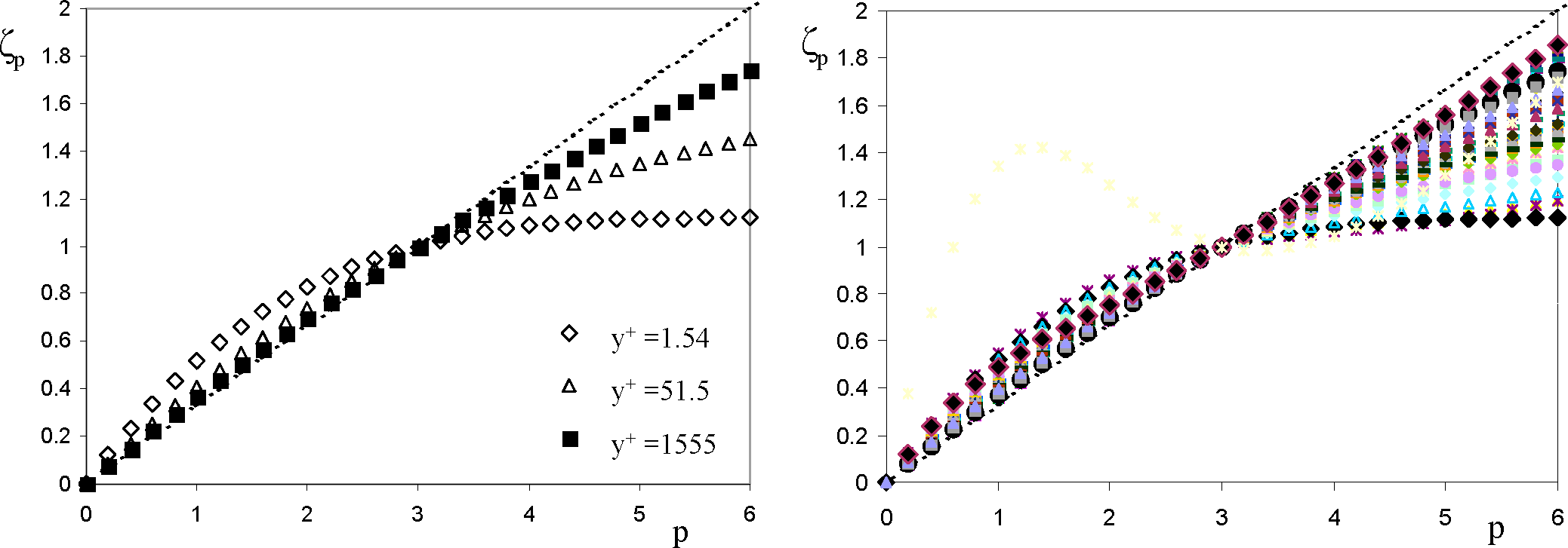
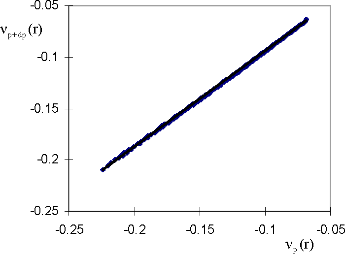
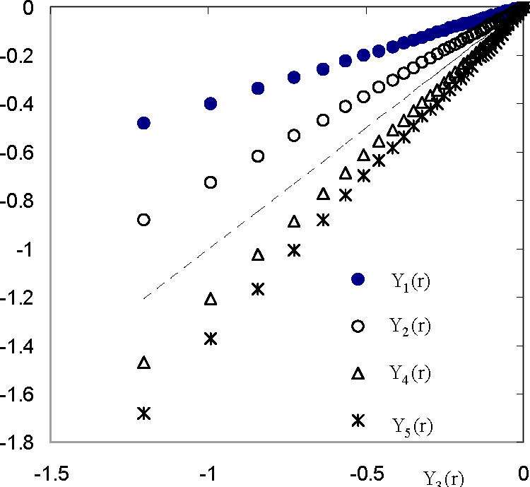
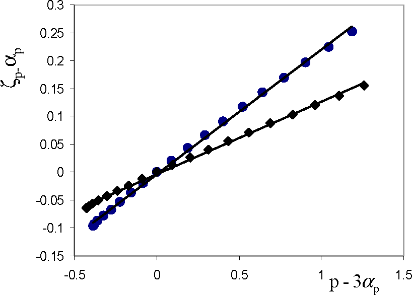
4.1. Scaling Exponents Measured by Extended Self-Similarity

To verify our geometrical approach and to compare it with the help of experimental data, we used a database obtained at Laboratoire de Mécanique de Lille and whose detailed description can be found in reference [30]. A set of 50 cases corresponding to 50 values of y⁺ ranging from 1–2722 has been considered. Each case is given by a signal staring from 6 × 10⁵–2.6 × 10⁶ points obtained by hot-wire anemometry. The studied flow has a mean velocity U_E = 3 m/s and corresponds to a boundary layer with zero pressure gradient. Its global thickness is δ = 0.35 m, the displacement thickness is δ* = 0.055 m, the momentum thickness is θ = 0.041 m. The von Kármán constant is κ = 0.41. The friction velocity is equal to u* = 0.11 m/s. We nondimensionalize δ: we have δ⁺ = (δu*)/ν. It gives δ⁺ = 2576. For each case, we determined the characteristic scales: Taylor scale λ and integral scale r₀. To define the velocity profile, the mean velocity U and turbulent intensity U’ as a function of y⁺ are also measured.

We calculated for each case the structure functions based on the velocity increments. We study the moments $\langle {\left|\delta V\right|}_{\mathrm{\Delta }t}{}^p\rangle$ based on the absolute value of velocity fluctuations ${\left|\delta V\right|}_{\mathrm{\Delta }t}=\left|V(t+\mathrm{\Delta }t)-V(t)\right|$ between two measurements separated by time increment Δt. To have the equivalent moments $\langle {\left|\delta V\right|}_r{}^p\rangle$ based on velocity fluctuation ${\left|\delta V\right|}_r=\left|V(x+r)-V(x)\right|$ between two points separated by a distance r, we used Taylor’s hypothesis i.e., r = UΔt where U is the mean longitudinal velocity for the position y⁺ which is investigated. We express our results with the non-dimensional scale coordinate ln(r/r₀) with r₀ = UΔt₀ where Δt₀ corresponds to the integral time. Integral and Taylor time-scales are measured by computing the auto-correlation function. The structure functions are computed for all the y⁺ values considered, i.e., for $1\le y^{+}\le 2722$. Let us introduce the non-dimensional quantity $Y_p(r)=\ln \left[\langle {\left|\delta V\right|}_r{}^p\rangle /\langle {\left|\delta V\right|}_{r_0}{}^p\rangle \right]$. We computed structure function for p ranging from 0.2–6 with an increment dp = 0.2. In Figure 1, we present the structure functions of orders 1, 2, 3, 4 and 5. The Taylor and integral scales are indicated by dashed lines. As expected, it can be observed that no real power law can be defined in the scale range [λ, r₀] which makes difficult any determination of the scaling exponents ζ_p.

In the absence of power laws, we used extended self-similarity in order to determine the relative exponents ζ_p/ζ₃. We give an example in Figure 2 for the case y⁺ = 51.3 but the same behaviour is followed for all the y⁺ range. More generally, we recall that extended self-similarity [8] consists in representing a moment of order p versus another one of order q leading to power laws. This gives the relative scaling exponents ζ_p/ζ_q. We focused on the relative scaling exponents ζ_p/ζ₃; using the exact result ζ₃ = 1 [3], we thus can determine the absolute scaling exponents.

We used the quantity Y_p(r) in order to be able to represent different values of p in the same graph. We verified that Y_p(r) is indeed a power law of Y₃(r). We determined the slope only in the scale range [λ, r₀] although the power law remains valid outside this scale range. In Figure 3, we present the scaling exponents ζ₁, ζ₂, ζ₄ and the quantity μ = 2 − ζ₆ classically used to characterize intermittency in the context of log-normal model [4]; the same kind of results are obtained for fractional orders. We recover the results already observed by several teams sharing that scaling exponents deviate increasingly from Kolmogorov behaviour when approaching the wall but we have a much larger range of y⁺ values here than the studies just quoted.

The evolution of ζ_P with wall distance displays two main zones separated at approximately y⁺ around 50. We can evidence two characteristic zones in these curves where scaling exponents seem to be constant while defining a plateau. The first one corresponds approximately to the range [300, 1500] and the second one approximately to the range [7, 50]. Let us analyze the first one. The value of scaling exponents of the first plateau is close to the set of values ζ_P^HI (indicated by a dashed-line) which correspond to a homogeneous and isotropic case. Nevertheless, this does not say anything about the intermittency efficiency and the crest dimension which should be introduced in the Equation (14) to calculate theoretically the exponents. We just recover values close to the ones of a homogeneous and isotropic flow but we emphasize the fact that this does not mean that the crest has a filamentary form (Δ_∞ = 1) and γ = 0.68. The experimental values γ and Δ_∞ will be measured just after. The second plateau ( $y^{+}\in$ [7,50]) corresponds to a much more intermittent configuration since the deviation from the Kolmogorov’s theory is much larger. As an indication, we represented (dotted line) the calculated values ζ_P^• for the couple (Δ_∞^• = 2 and γ^• = 0.36). For y⁺ > 1500, we have a more intermittent behaviour. The same results have been obtained for the fractional order structure functions. We thus recover the same qualitative result of references [12] and [13] which have also found two characteristic zones for intermittency, an “homogeneous” one (y⁺ = 310 in [12] and y⁺$\ge$ 100 in [13]), and a more intermittent one ( $10\le y^{+}\le 40$ in [12] and 20 ≤ y⁺ ≤ 50 in [13]) which corresponds approximately to the buffer layer.

In Figure 4, we present the evolution scaling exponents ζ_P as a function of p for several values of ranging from 1–2722: we recall that ζ_P/ζ₃ is measured and we use ζ₃ = 1 to have ζ_P. It is observed that, when the wall distance decreases, the curve displays a tendency to saturate. In these cases, the saturation can be noticed starting from the value p = 4. Let us note that this kind of saturation has also been obtained in the study of intermittency of a passive scalar such as temperature, for scaling exponents extracted from the corresponding scalar structure functions [31,32]. A good model of intermittency for wall turbulence must thus be able to describe the double dependency of scaling exponents on order and wall distance, and namely their tendency to saturate near the viscous layer.

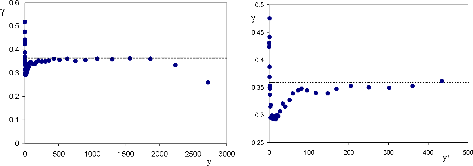
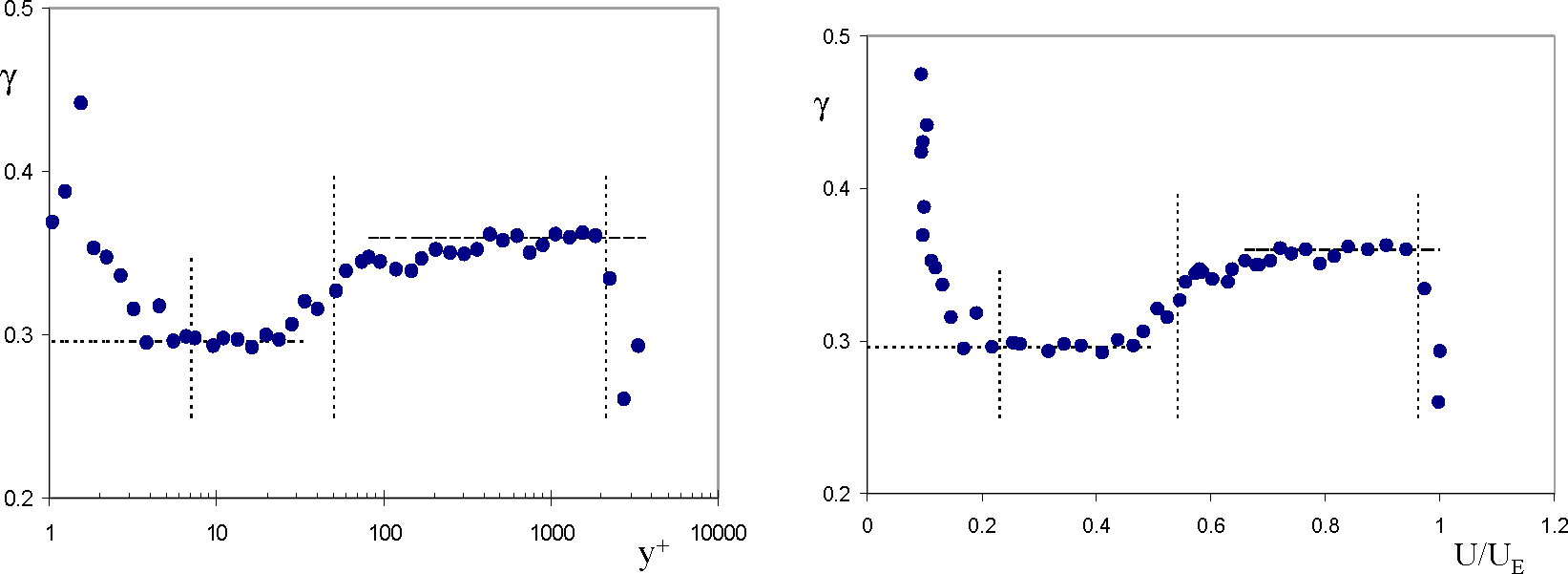
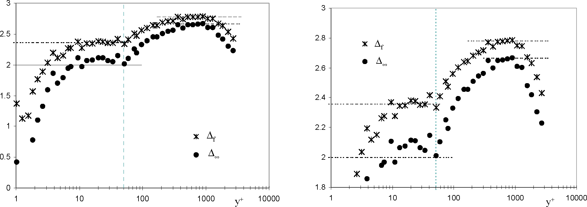
4.2. Intermittent Efficiency, Bulk and Crest Dimensions

To determine the intermittency efficiency γ, we used computed structure functions based on the velocity increments and namely the expression ${\nu }_{p+dp}(r)={\overline{\delta V_r}}^{1-\mathrm{\Gamma }}{\nu }_p{(r)}^{\mathrm{\Gamma }}{}_{}$ where $\mathrm{\Gamma }={\gamma }_v{}^{dp}$, an expression linking the relative structure functions. At fixed scale between Taylor and integral scale, we represent ${\nu }_{p+dp}(r)$ as a function of ${\nu }_p(r)$ for values of p ranging from 1–5 (here dp = 0.2). We verified that this leads to power laws. We did this for different scales from Taylor scale to integral scale. In Figure 5, an example of the resulting curve is shown; we obtained a perfect power law. To have Γ we just fit through the data: then we calculate γ_v with $\mathrm{\Gamma }={\gamma }_v{}^{dp}$ and finally γ with ${\gamma }_v={\gamma }^{1/3}$. The power law behaviour is well verified for all our range of y⁺ values.

Having determined each y⁺ value, we obtained the variation of γ with wall distance (Figure 6). For small values of y⁺ (Figure 6, right), the curve looks like a sort of potential interaction. It has a minimum at γ_m = 0.297 around y⁺_m ≈ 12. This can be linked to the fact that, in a turbulent boundary layer, y⁺ = 12 corresponds to the maximal production of kinetic energy. When y⁺ increases, γ tends towards a value close to 0.36 (predicted by ESG).

To evidence particular zones in the evolution of γ, we represent it with a logarithmic abscissa (Figure 7, left) for y⁺ and as a function of U/U_E (Figure 7, right). Again the curve is composed of two main, apparently symmetrical parts. For y⁺ > 2100, the intermittency is strong and is relative to outer intermittency since this zone corresponds to the outer region. For 300 ≤ y⁺ ≤ 2100, intermittency efficiency is relatively constant and is close to the value 0.36. It decreases until a minimal value around 0.297. The intermittency efficiency is constant, equal to 0.297 in the range 7 < y⁺ ≤ 24. For y⁺ ≤ 7, it increases towards values around 0.42 but with high uncertainty. We thus recover for the region 300 ≤ y⁺ ≤ 2100, the value γ^• = 0.36. We found a second plateau for 7 < y⁺ ≤ 24 where intermittency is much larger (indicated by scaling exponents, see Figure 7) but intermittent efficiency is slightly smaller than the theoretical value 0.36.

In order to determine the bulk dimension Δ_f, we used Equation (17) i.e., ${\zeta }_p-{\alpha }_p={\chi }_v{(p-3{\alpha }_p)}_{}{}^{}with{}^{}{\alpha }_p=(1-{\gamma }^{p/3})/(1-\gamma )$ where χ_v = (Δ_f − 2)/3. We represent ${\zeta }_p-{\alpha }_p$ as a function of $p-3{\alpha }_p$ for p varying from 1–5. As an illustration, we give, in Figure 8, the case corresponding to y⁺ = 350 and y⁺ = 31. The same property is obtained for all the y⁺ values and gives us the possibility to determine the quantity χ_v and thus Δ_f.

Using the intermittency efficiency and the value of χ_v as a function of wall distance, the bulk and crest dimension are calculated. To be physically coherent, we expect to find values of fractal dimension between 0 and 3 and a particular behaviour for Δ_∞ = 2. The results are shown in the Figure 9. Again the value y⁺ = 50 is remarkable since it divides the curve into two main seemingly convex zones. A plateau can be observed for values of y⁺ in [360, 1100] where bulk dimension reaches a maximum: Δ_f,M = 2.78, the corresponding crest dimension being Δ_{∞, M} = 2.66 (in this region γ = γ^• = 0.36). A second plateau can be distinguished for values of y⁺ in [7, 40] (corresponding to the buffer layer) with a seemingly constant value noted Δ_f,M,I close to 2.36. The corresponding crest is around 2.08 (in coherence with the fact that in this region γ = 0.3). For values around y⁺ = 50, the curve seems to present a crest dimension decreasing towards 2 just before increasing again. Nevertheless, in this region, uncertainties in measurements do not allow making a conclusion. We can also observe the fact that for a value of y⁺ of around 7, the crest dimension becomes smaller than 2. This implies that, for values y⁺ > 7 i.e., beyond the viscous layer, crest and bulk dimension values are larger than two. Values of fractal dimension smaller than 2 (dimension of the wall) occur on the viscous layer. This is consistent with the idea that viscous layer appears for the boundary layer as a sheet-like structure.

The intermittency efficiency vary in the viscous layer (y⁺ < 7) and approaching the external border of the boundary layer (y⁺ > 2100); nevertheless, in a wide range of y⁺ values (i.e., 7 ≤ y⁺ ≤ 2100), its variations remain very small recalling the fact that γ can vary between 0 and 1: γ is varying between 0.3 and 0.36 with a transition between these two values centered at y⁺ = 50. It would thus be interesting to give a simplified model in order to describe all the set of curves obtained experimentally. Let us consider a value constant to 0.36 (this value is also justified by some theoretical arguments) and let us make vary the crest dimension from 2.6 to 1 (Figure 10). The scaling exponents calculated with Expression (14) lead to the same general set of curves obtained experimentally and we also described the tendency toward saturation. Nevertheless, to be complete and to really be able to compare our model to experimental data, a link between crest dimension and wall-distance defined by y⁺ is missing. We expect to develop this point in the future.

5. Conclusions

In order to describe the phenomenon of intermittency in wall bounded turbulence such as a turbulent boundary layer, we introduced a new geometrical framework based on scale-entropy and a hierarchy of fractal sets (the “entropic skins”) linked to each other by scale-entropy dynamics which is characterized by intermittency efficiency. Two extrema are important: the bulk and the crest with $\gamma =({\mathrm{\Delta }}_f-{\mathrm{\Delta }}_{\infty })/(d-{\mathrm{\Delta }}_{\infty })$. We found that the scaling exponents usually defined in turbulence take the general form ${\zeta }_p=\left[({\mathrm{\Delta }}_{\infty }(1-\gamma )+3\gamma -2)/3\right]p+(3-{\mathrm{\Delta }}_{\infty })(1-{\gamma }^{p^{-}/3})$; Δ_∞ and γ are parameters depending on the experimental conditions and/or the distance to the wall.

We verified in an experimental boundary layer the interest of our approach for a wide range of wall distances ( $1\le y^{+}\le 2722$). Using extended self-similarity, we measured the scaling exponents which vary with y⁺ and display a tendency to the saturation in the vicinity of the wall, a behaviour which is captured by our model. Intermittency efficiency displays a complex behaviour when it is looked in detail but, in the whole boundary layer, it varies slightly and remains between 0.3 (corresponding to the buffer layer) and 0.36 in the inertial layer. Our theoretical and experimental results show that entropic-skins geometry based on conceptual but simple geometrical arguments can describe intermittency features of wall turbulence. One important advantage of our model is to establish a direct link between multi-scale features and statistics usually defined in this field such as structure functions and scaling exponents. Our geometrical framework is quite general and could be applied to a wide variety of systems involving multi-scale and complex scaling features.

References

1. Kolmogorov, A.N. The local structure of turbulence in incompressible viscous fluid for very large Reynolds numbers. Doklady Akademii Nauk SSSR 1941, 30, 9–13. [Google Scholar]
2. Kolmogorov, A.N. On degeneration (decay) of isotropic turbulence in an incompressible flow. Doklady Akademii Nauk SSSR 1941, 32, 538–540. [Google Scholar]
3. Anselmet, F.; Gagne, Y.; Hopfinger, E.J.; Antonia, R.A. High-order velocity structure functions in turbulent shear-flows. J. Fluid Mech 1984, 140, 63–89. [Google Scholar]
4. Kolmogorov, A.N. A refinement of previous hypotheses concerning the local structure of turbulence in a viscous incompressible fluid at high Reynolds numbers. J. Fluid Mech 1962, 13, 82–85. [Google Scholar]
5. Frisch, U.; Sulem, P.L.; Nelkin, M. A simple dynamical model of intermittent fully developed turbulence. Fluid Mech 1978, 87, 719–736. [Google Scholar]
6. Frisch, U. Turbulence: The Legacy of A.N. Kolmogorov.; Cambridge University Press: Cambridge, UK, 1995. [Google Scholar]
7. She, Z.-S.; Lévêque, E. Universal scaling laws in fully developed turbulence. Phys. Rev. Lett. 1994, 72, 336–339. [Google Scholar]
8. Benzi, R.; Ciliberto, S.; Tripiccione, R.; Baudet, C.; Massaioli, F.; Succi, S. Extended self-similarity in turbulent flows. Phys. Rev. E 1993, 48, R29–R32. [Google Scholar]
9. Dubrulle, B. Intermittency in fully developed turbulence: Log-Poisson statistics and generalized scale covariance. Phys. Rev. Lett. 1994, 73, 959–962. [Google Scholar]
10. Protas, B.; Goujon-Durand, S.S.; Wesfreid, J.E. Scaling properties of two-dimensional turbulence in wakes behind bluff bodies. Phys. Rev E 1997, 55, 4165–4169. [Google Scholar]
11. Gaudin, E.; Protas, B.; Goujon-Durand, S.; Wojciechowski, J.; Wesfreid, J.E. Spatial properties of velocity structure functions in turbulent wake flows. Phys. Rev. E 1998, 57, R9–R12. [Google Scholar]
12. Onorato, M.; Camussi, R.; Iuso, G. Small scale intermittency and bursting in a turbulent channel flow. Phys. Rev. E 2000, 61, 1447–1454. [Google Scholar]
13. Toschi, F.; Amati, G.; Succi, S.; Benzi, R.; Piva, R. Intermittency and structure functions in channel flow turbulence. Phys. Rev. Lett. 1999, 83, 5044–5047. [Google Scholar]
14. Sreenivasan, K.R. Fractals and multifractals in fluid turbulence. Ann. Rev. Fluid Mech 1991, 23, 539–604. [Google Scholar]
15. Sreenivasan, K.R.; Ramshankar, R.; Meneveau, C. Mixing, entrainment and fractal dimensions of surfaces in turbulent flows. Proc. R. Soc. Lond. A 1989, 421, 79–108. [Google Scholar]
16. Vassilicos, C.; Hunt, J. Fractal dimensions and spectra of interfaces with application to turbulence. Proc. R. Soc. Lond. A 1991, 435, 505–534. [Google Scholar]
17. Catrakis, H.J.; Dimotakis, P.E. Mixing in turbulent jets: scalar measures and isosurface geometry. J. Fluid Mech 1996, 317, 369–406. [Google Scholar]
18. Pocheau, A.; Queiros-Conde, D. Scale covariance of the wrinkling law of turbulent propagating interfaces. Phys. Rev. Lett. 1996, 76, 3352–3355. [Google Scholar]
19. Queiros-Conde, D. A diffusion equation to describe scale- and time-dependent dimensions of turbulent interfaces. Proc. R. Soc. Lond. A 2003, 459, 3043–3059. [Google Scholar]
20. Vincent, A.; Meneguzzi, M. The spatial structure and statistical properties of homogeneous Turbulence. J. Fluid Mech 1991, 225, 1–20. [Google Scholar]
21. Douady, S.; Couder, Y.; Brachet, M.E. Direct observation of the intermittency of intense vorticity filaments in turbulence. Phys. Rev. Lett. 1991, 67, 983–988. [Google Scholar]
22. Queiros-Conde, D. Geometry of intermittency in fully developed turbulence. C. R. Acad. Sci. IIB 1999, 327, 1385–1390. [Google Scholar]
23. Queiros-Conde, D. Entropic-skins model of fully developed turbulence. C. R. Acad. Sci. IIB 2000, 328, 541–546. [Google Scholar]
24. Ruiz Chavarria, G.R.; Baudet, C.; Ciliberto, S. Hierarchy of the Energy Dissipation Moments in Fully Developed Turbulence. Phys. Rev. Lett. 1995, 74, 1986–1989. [Google Scholar]
25. She, Z-S.; Waymire, E.C. Quantized energy cascade and log-Poisson statistics in fully developed turbulence. Phys. Rev. Lett. 1995, 74, 262–265. [Google Scholar]
26. Benzi, R.; Biferale, L.; Trovatore, E. Universal statistics of non-linear energy transfer in turbulent models. Phys. Rev. Lett. 1995, 77, 3114–3117. [Google Scholar]
27. Müller, W.-C.; Biskamp, D. Scaling properties of three-dimensional magnetohydrodynamic turbulence. Phys. Rev. Lett. 2000, 84, 475–478. [Google Scholar]
28. Liu, L.; She, Z.-S. Hierarchical structure description of intermittent structures of turbulence. Fluid Dyn. Res. 2003, 33, 261–286. [Google Scholar]
29. Queiros-Conde, D. Internal symmetry in the multifractal spectrum of fully developed Turbulence. Phys. Rev. E 2001, 64, 015301(R). [Google Scholar]
30. Carlier, J.; Stanislas, M. Experimental study of eddy structures in a turbulent boundary layer using particle image velocimetry. J. Fluid Mech 2005, 535, 143–188. [Google Scholar]
31. Celani, A.; Lanotte, A.; Mazzino, A.; Vergassola, M. Universality and Saturation of Intermittency in Passive Scalar Turbulence. Phys. Rev. Lett. 2000, 84, 2385–2388. [Google Scholar]
32. Moisy, F.; Willaime, H.; Andresen, J.S.; Tabeling, P. Passive Scalar Intermittency in Low Temperature Helium Flows. Phys. Rev. Lett. 2001, 86, 4827–4830. [Google Scholar]
Figure 1. Structure functions: ln | δ V | r p vs. ln(r/r0) for y+ = 51.5. The Taylor and the integral scales are indicated by vertical dashed lines.
Entropy 17 02198f1
Figure 2. Extended self-similarity at y+ = 51.5 for scale r such as λ r r 0: Yp(r) vs. Y3(r) for p = 1, 2, 4, 5. The dashed line correspond to the trivial case Y3(r). The slope gives relative scaling exponents ζp/ζ3. The absolute scaling exponents are calculated using the exact result ζ3 = 1.
Entropy 17 02198f2
Figure 3. Experimental scaling exponents (measured by ESS) vs. y+ logarithmic coordinate: (a) ζ1 vs. y+; (b) ζ2 vs. y+; (c) ζ4 vs. y+; (d) μ = 2 − ζ6 vs. y+. The dashed-lines gives the values corresponding to the homogeneous and isotropic case ζ1HI = 0.36, ζ2HI = 0.70, ζ4HI = 1.28 and μHI = 0.23. The dotted-lines corresponds to exponents calculated with Equation (14) for γ = 0.36 and Δ = 2, ζ1 = 0.408, ζ2 = 0.734, ζ4 = 1.223 and μ = 0.41. The value y+ = 50 separates the curve in two main parts.
Entropy 17 02198f3
Figure 4. (Right) Experimental scaling exponents (measured by ESS) ζP vs. p for y+ = 1.54; y+ = 51.5; y+ = 1555; The dashed line indicates Kolmogorov’s linear law. (Left) Scaling exponents ζP for y+ values ranging from to 1–2722.
Entropy 17 02198f4
Figure 5. Example of measurement of γ. ν p + d p ( r ) as a function of ν p ( r ) (here dp = 0.2) for values of p ranging from 1–5 (y+ = 51.5); slope Γ = 0.928, i.e., γ = 0.326.
Entropy 17 02198f5
Figure 6. (Left) Intermittency factor γ vs. y+; (Right) zoom on the range [1, 500]; Dashed line indicates the theoretical value γ = 0.36.
Entropy 17 02198f6
Figure 7. (Left) Measured reversibility efficiency γ vs. y+ (logarithmic coordinate); Horizontal dashed line the theoretical value γ = 0.36. (Right) Intermittency factor γ vs. U/UE. Vertical dashed lines indicates the values corresponding to y+ = 7, 50 and 2100.
Entropy 17 02198f7
Figure 8. Measurement of Δf. Quantity ζ p α p as a function of p 3 α p for p varying from 1–5. Two examples: the disks correspond to y+ = 350: the linear fit gives χv = 0.223 i.e., Δf = 2.67; the rhombs correspond to y+ = 31: the linear fit gives χv = 0.1305 i.e., Δf = 2.39 with χv = (Δf − 2)/3).
Entropy 17 02198f8
Figure 9. (Left) Bulk and crest dimensions Δf and Δ vs. y+ in logarithmic coordinate; (Right) Zoom on the superior part; dashed lines represents the values 2.36, 2.66 and 2.78. A singular point at y+ = 50 links two seemingly convex parts. It corresponds to the case γ = 0.36, Δ = 2 and Δf = 2.36. The crest dimension becomes smaller than 2 at around y+ = 7.
Entropy 17 02198f9
Figure 10. Calculation of scaling exponents with Expression (14): ζ p = [ ( Δ ( 1 γ ) + 3 γ 2 ) / 3 ] p + ( 3 Δ ) ( 1 γ p / 3 ) for crest dimension taking the values 2.6, 2.4, 2.2, 2, 1.8, 1.6, 1.4, 1.2 and 1. The intermittency efficiency is kept constant γ = γ = 0.36. Dotted line corresponds to the K41 theory. The bold curve corresponds to the case Δ = 2.
Entropy 17 02198f10