Distributed Extreme Learning Machine for Nonlinear Learning over Network


Department of Information Science and Electronic Engineering, Zhejiang University, Hangzhou 310027, China
*
Author to whom correspondence should be addressed.
Entropy 2015, 17(2), 818-840; https://doi.org/10.3390/e17020818
Submission received: 26 December 2014
/
Revised: 20 January 2015
/
Accepted: 6 February 2015
/
Published: 12 February 2015
(This article belongs to the Special Issue Recent Advances in Chaos Theory and Complex Networks)
Abstract
:Distributed data collection and analysis over a network are ubiquitous, especially over a wireless sensor network (WSN). To our knowledge, the data model used in most of the distributed algorithms is linear. However, in real applications, the linearity of systems is not always guaranteed. In nonlinear cases, the single hidden layer feedforward neural network (SLFN) with radial basis function (RBF) hidden neurons has the ability to approximate any continuous functions and, thus, may be used as the nonlinear learning system. However, confined by the communication cost, using the distributed version of the conventional algorithms to train the neural network directly is usually prohibited. Fortunately, based on the theorems provided in the extreme learning machine (ELM) literature, we only need to compute the output weights of the SLFN. Computing the output weights itself is a linear learning problem, although the input-output mapping of the overall SLFN is still nonlinear. Using the distributed algorithm to cooperatively compute the output weights of the SLFN, we obtain a distributed extreme learning machine (dELM) for nonlinear learning in this paper. This dELM is applied to the regression problem and classification problem to demonstrate its effectiveness and advantages.
1. Introduction
Due to the rapid development and broad application of networks of small, low-power devices that can sense, process and communicate information about their environment, e.g., wireless sensor networks (WSN), distributed data processing has become a hot topic in recent years. We start by considering a specific learning task regression, which is an efficient framework for data modeling. Distributed regression is to collaboratively learn the mapping between the input and the output based on noisy measurements collected at nodes distributed over a geographic region [1–5]. In the distributed implementations, the communication only occurs among one-hop neighboring nodes, which will help save energy and bandwidth [6,7]. Different types of distributed algorithms, including the diffusion type [1] and the consensus type [4], were developed for the distributed regression problem.
In previous studies, most of the existing distributed algorithms were developed for linear regression problem. These distributed algorithms succeeded in a number of cases where the measurements can be well modeled using a linear data model with additive noise [1]. However, in some real-world environments, the input-output relationship might be a nonlinear function f. In these cases, it is obviously unsuitable to collaboratively solve the nonlinear regression problems using the existing distributed linear algorithms directly.
Based on the solid mathematical foundation and considerable experimental successes, the kernel method was frequently adopted in centralized nonlinear learning [8,9]. Notice that in the standard kernel method, a learned function depends on all of the data
. However, communication is usually the biggest energy-consuming factor in WSN, which precludes an individual node from accessing the entire dataset and, thus, prevents one from using the kernel-based learning algorithms for distributed nonlinear regression directly.
Based on the successive orthogonal projection (SOP) algorithm [10], in [11,12], a distributed kernel least squares regression algorithm was recently proposed. This algorithm is proven to be effective for the nonlinear regression problem, but it has several flaws [13]. First, this algorithm is not an online learning algorithm, which hinders the ability to perform real-time estimation and adaptation in the case of the continuous streaming of measurements. Confined by the procedure of the SOP algorithms, we cannot simultaneously train several nodes if they share exemplars in their locally accessible training datasets. Besides, as to the robustness, if one individual node in the network stops working, then the whole learning algorithm cannot go on, which will lead to a catastrophic failure of the learning task. However, one of the purposes of developing distributed algorithms is to keep the holistic network working in spite of the individual node and/or link failure. In addition, each node has to broadcast their measurements to their neighboring nodes, which increases the communication burden. A modification of this distributed kernel algorithm was presented in [13]. This modified algorithm has a lower communication burden and allows asynchronous computation. However, it is still off-line, and each node also has to broadcast their measurements to their neighboring nodes.
Another broadly-used nonlinear modeling tool is the neural network. The multilayer perceptron (MLP) is the first attempt, but there are multilayer weight parameters to be estimated and communicated. The radial basis function (RBF) neural networks with Gaussian functions have been broadly used in the nonlinear regression problem [14]. Notice that we need to determine the centers and widths of the Gaussian basis functions based on the entire training set when we train the RBF neural networks. However, in distributed learning, the constraints on energy and communication preclude individual nodes from accessing the entire training set, which leads to the difficulty in adopting the distributed version of the usual learning algorithm to train the neural network directly.
In recent years, the extreme learning machine (ELM) was proposed [15–17]. In the ELM theory, it was proven mathematically that the hidden neurons of the single hidden layer feedforward neural network (SLFN) do not need to be tuned. With the randomly-generated parameters of the hidden layer and properly chosen output weights, the SLFN can approximate any continuous target function [18]. Thus, in the SLFN with RBF hidden neurons, we can just randomly select the centers and the widths and, then, only calculate the output weights [18]. From this point of view, training the output weights of the SLFN based on the ELM algorithm can be simply viewed as a linear learning problem. However, SLFN’s ability to construct nonlinear mapping between the input and the output is unchanged. Thus, we use the distributed algorithm to cooperatively train the output weights of the SLFN, which results in distributed ELM for the distributed nonlinear regression problem. In the above discussions, this distributed ELM is motivated for the nonlinear regression problem, which learns the relationship between the input and the output. There are many other problems that can also be formulated as constructing the input-output relationship, for example the classification problem. The centralized ELM algorithm was applied to the classification problem [18]. In this paper, we also apply the distributed ELM to the classification problem. The application scope of the distributed ELM is beyond regression and classification; we thus use nonlinear learning to denote the general applicability. In this paper, we only consider the SLFN with RBF hidden neurons. The training and performance of the SLFN with the sigmoidal activation function are quite similar to those of the RBF one.
One of the key advantages of the distributed ELM, among others, is its simplicity, which is especially important, considering the limited computational resources in WSNs.
This paper is organized as follows. In Section 2, some preliminaries about the nonlinear data model, the SLFN and the ELM algorithm are presented. Then, several types of distributed ELM algorithms are formulated in Section 3. In Section 4, a number of application examples for both regression and classification problems are presented to demonstrate the effectiveness and advantages of the new algorithms. Finally, conclusions are drawn in Section 5.
2. Preliminaries
2.1. Distributed Nonlinear Model
We consider a sensor network consisting of N nodes, which are distributed over a geographic region. At each time instant i, each node k has access to the measurement {dk(i),uk,i} of the zero-mean random process {dk(i), uk,i}, where dk(i) and uk,i are the 1 × m vector and the 1 × n vector, respectively.
Although the linear data model used in most of the existing distributed learning literature has the ability to capture many cases of interests, there are still many situations beyond the range of the linear data model. In the nonlinear case, we assume that the data model is described by:
where vk(i) is the background noise with variance
, and
can be different for different nodes. The regressor uk,i is assumed to be spatially independent for each node k and independent identically distributed (i.i.d.) in time. The same assumption in time and space is made for the measurement noise vk(i). In addition, uk,i is assumed to be independent of vk(i).
Given the data model (1), our object is to learn the unknown nonlinear function of interest f from the noisy measurements {dk(i),uk,i} at each node in the network. In distributed learning, each node k in the network only communicates with its one-hop neighboring nodes, denoted by Nk (including k).
2.2. SLFNand ELM Algorithm
For nonlinear learning, the ELM algorithm developed for the SLFN received a lot of attention due to its simplicity and superior performance. In the ELM theory, it is demonstrated that for ELM based on various types of hidden neurons, all can approximate any continuous target function with zero error, when the number of hidden nodes tends to infinity [19]. For the classification ability of the ELM, if the output of the SLFN based on the ELM is dense in C(Rd), this SLFN can classify arbitrary disjoint regions of any shapes in Rd [19]. Here, C(Rd) denotes the class label. For different types of hidden neurons, the performance of the SLFN is quite similar for each. Moreover, the SLFN with the RBF hidden neurons was successfully used in many contexts [18]. In this paper, we just consider the RBF hidden neurons as representative. In the following discussion, we first describe the SLFN with the RBF hidden neuron used in this paper; then, we review the ELM algorithm briefly.
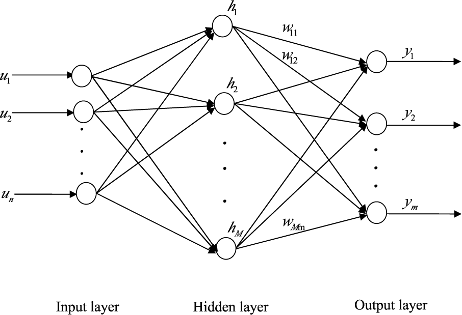
An SLFN with n neurons in the input layer, M RBF neurons in the hidden layer and m neurons in the output layer, as shown in Figure 1, is considered in most of the ELM algorithms. Given N pairs of samples (di,ui), i = 1,…, N, for arbitrary i-th input vector ui, the input-output relationship of the SLFN with M hidden neurons is given by:
where ui = [ui1,…, uin] is the i-th input vector; g is the Gaussian activation function; bj = [bj1,…, bjn] and δj are the center and the impact width of the j-th Gaussian activation function, respectively; hi = [hi1,…, hiM] is the output vector of the hidden layer with respect to input xi ; and W = [w1,…, wm]t is the M × m weight matrix connecting the hidden layer to the output layer.
Based on the theorems in [16], we just need to randomly select M kernel centers b = [b1,…, bm]t and M impact widths δ = [δ1,…, δm] drawn from any continuous probability distribution and fix them. Given N arbitrary samples
, under the assumption that the SLFN can approximate the input-output relationship of these N measurements with zero error, then we can obtain N equations. For the propose of the simplicity of expression, we present a compact form of these equations, which is defined as:
where:
Notice that the hidden layer output matrix H actually remains unchanged in batch mode.
There are a number of approaches to compute the value of W [17], such as the orthogonal projection method, the iterative method and singular value decomposition (SVD) [20]. If the matrix HT H is nonsingular, a smallest norm least-squares solution can be obtained for the above linear equation (3). In this case, the solution is given by:
where H† is the Moore-Penrose generalized inverse [20] of matrix H. If HT H is singular, the SVD is usually adopted to compute H† in the batch ELM algorithm.
In real-world applications, the measurement may keep streaming in. In this case, by extending the ELM algorithm to online learning, the online sequential ELM (OS-ELM) algorithm [17] was presented. Two phases, including an initialization phase and a sequential learning phase, are necessary for this OS-ELM algorithm. The OS-ELM algorithm was investigated in detail in [17]. We omit the description of this algorithm here.
3. Distributed ELM for Nonlinear Learning
The diffusion type of distributed algorithm is not only able to respond in real time based on operating over a single time scale, but also robust to node and/or link failure [21]. Owing to these merits, this type of distributed algorithm was widely investigated for distributed learning, such as diffusion least-mean squares (LMS) [1,22,23], diffusion information theoretic learning [5], diffusion sparse LMS [24], diffusion recursive least-squares (RLS) [25,26] and diffusion sparse RLS [27]. In this paper, we use the diffusion LMS algorithm and the diffusion RLS algorithm to adaptively adjust the output weights of the SLFN with RBF hidden neurons, which leads to the distributed ELM based on the diffusion least-mean squares (dELM-LMS) algorithm and the distributed ELM based on the recursive least-squares (dELM-RLS) algorithm, respectively.
In these distributed ELM algorithms, the SLFN shown in Figure 1 is used to learn the unknown nonlinear function at each node k in the sensor network. We assume that the training data arrives one-by-one. Thus, at each time i, given the input uk,i for each node k, the corresponding output of this node is:
where hk,i = [hk,i1,…, hk,im] is the output vector of the hidden layer with respect to the input uk,i of node k. For different RBF hidden neurons of the SLFN in one node, we use different centers and impact widths. For the SLFNs used at different nodes in the network, we use the same sets of centers and impact widths. In the following discussions, we first give the derivation of dELM-LMS algorithm. After that, we present the derivation of dELM-RLS algorithm. Notice that there are some differences between the derivation of the distributed ELM algorithms in this paper and that of the diffusion LMS and RLS algorithms in the literature [1,22,23,25,26], so we present the derivation in detail.
3.1. Distributed ELM-LMS
In the dELM-LMS algorithm, for each node k in the sensor network, the local cost function is defined as a linear combination of local mean square error (MSE), that is:
where W is the output weight matrix of the SLFN, hl,i is the output vector of the hidden layer with respect to the input ul,i of the node l ∈ Nk and {clk} are the non-negative cooperative coefficients satisfying clk = 0 if l ∉ Nk, 1TC = 1T and C1 = 1. Here, C is an N × N matrix with individual entries {clk}, and 1 is an N × 1 vector whose entries are all unity. The cooperative coefficient clk decides the amount of the information provided by the node l ∈ Nk to node k and stands for a certain cooperation rule. In distributed algorithms, we can use different cooperation rules, including the Metropolis rule [28], the adaptive combination rule [29,30], the Laplacian matrix [31] and the relative degree rule [1]. In this paper, we use the Metropolis rule as the cooperation rule, which is expressed as:
where nk and nl are the degrees (numbers of links) of nodes k and l, respectively.
Given the local cost function for each node k in the network, the steepest descent method is adopted here. The derivative of (8) is:
Based on the steepest gradient descent method, at each time i, for each node k, we update the output weight matrix of the SLFN using:
where Rl,h and Rl,dh are the auto-covariance matrix of h and the cross-covariance matrix of h and d at node l, respectively, Wk,i is the estimate of the output weight matrix of node k at time i and μ is the step size. As we adopt the LMS type algorithm, namely an adaptive implementation, we can just replace these second-order moments by instantaneous approximations, that is:
By substituting (12) into (11), we obtain:
In order to compute Wk,i defined in (13), we need to transmit the original data {dl(i), hl,i} of all nodes l,l ∈ Nk to node k at each time i. We should notice that it brings a considerable communication burden to transmit the original data of all neighbor nodes of each node k at each time i. To tackle this issue, as in the diffusion learning literature [1,5], in this paper, we introduce an intermediate estimate. At time i, we denote the intermediate estimate at each node k by φk,i. We then broadcast the intermediate estimate φk,i to the neighbors of node k. At time i, for each node k, the local estimate expressed by the intermediate estimates of its neighbors can be written as:
We now give some remarks on the rationality for doing so. First, the intermediate estimate contains the information of measurements. In addition, transmitting the measurements of neighboring nodes does not provide a significantly better performance. Thus, we do not need to transmit the measurements. Besides, we can update the intermediate estimate for each node k at each time instant, but do not transmit the intermediate estimate at each time instant, which will further significantly reduce the communication burden. Although we transmit the intermediate estimate at each time instant in this paper, the performance of the dELM-LMS algorithm transmitting the intermediate estimate periodically (with a short period) is quite similar.
Substituting Equation (14) into Equation (15), we can derive an iterative formula for the intermediate estimate, that is:
As Wk,i-i is not available at node l, l ∈ Nk \ {k}, we cannot compute the value of the intermediate estimate of node l by the above equation. Similar to [5], we replace Wk,i–1 in the above equation by Wl,i–1, which is available at node l. Thus, we obtain:
The simulation results demonstrate the effectiveness of this replacement. In addition, detailed statements about the rationality of this replacement are presented in [5]. In this paper, we omit it for simplicity.
We replace the intermediate estimate φl,i–1 in the above equation by Wl,i–1, which is based on the following several facts. From (14), we know that Wl,i–1 is the linear combination of φl,i–1; thus, Wl,i–1 contains more information than φl,i–1 [1,32], and it has already been demonstrated that such a replacement in the diffusion LMS can improve the learning performance. Moreover, the vectors Wl,i–1 and φl,i–1 are both available at the node l. Based on this replacement and performing the “adaptation” step first, we acquire the two-step iterative update formula of the adapt-then-combine (ATC) type.
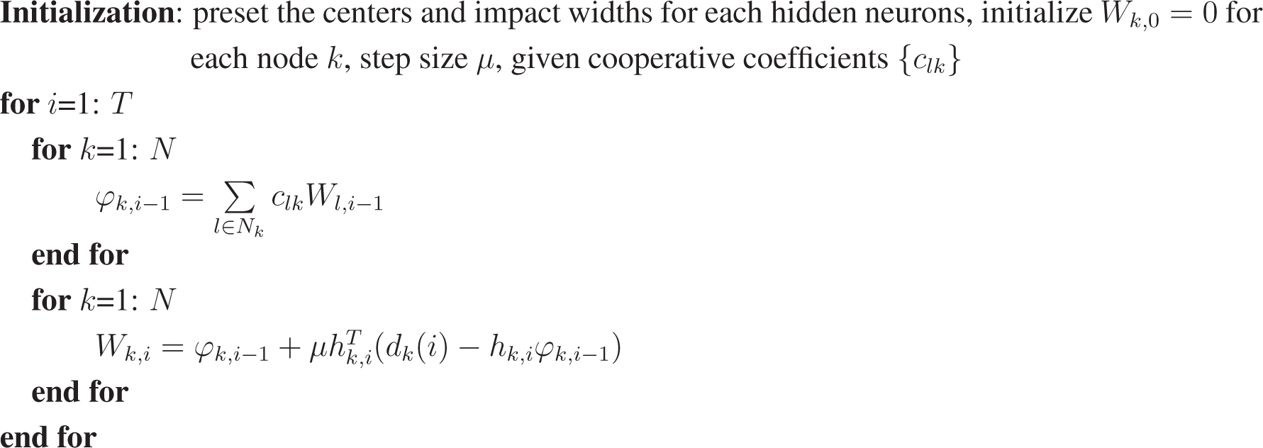
ATC dELM-LMS:
Alternatively, in each iteration, we can perform the “combination” step first, which leads to a combine-then-adapt (CTA)-type update formula. In the following, we sketch the derivation of this type of update formula.
From the discussion in the above, we know that
. In addition, Wk,i–1 is independent of
. Thus, we can multiply the first Wk,i–1 on the right-hand side of (13) by
. Then, substituting (14) into the left-hand side of (13), we can get:
Based on the above equation, it is immediate to obtain another iterative formula for φl,i, which is:
Similarly, we replace Wk,i–1 in (20) by Wl,i–1, leading to:
The two-step iterative formula is:
From the above derivation, we know that Wk,i and φl,i are the intermediate estimate and the local estimate for node k at time i, respectively. In order to avoid causing notational confusion, we exchange the notations of W and φ. Consequently, we obtain the two-step CTA-type iterative formula.
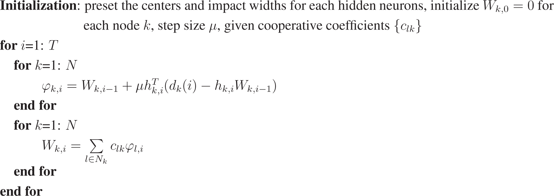
CTA dELM-LMS:
For the purpose of clarity, the procedure of the ATC dELM-LMS algorithm and the CTA dELM-LMS algorithm are summarized in Algorithm 1 and Algorithm 2, respectively.

 |
 |
Remark 1. In the dELM-LMS algorithm, the local cost function of node k can also be defined as a linear combination of the modified local MSE [1],
where {blk} are non-negative coefficients satisfying the conditions blk = 0 if l ∉ Nk and
, and φl is the intermediate estimate available at node l. After similar derivation as that performed in the dELM-LMS algorithms, we can obtain the more general two-step update equation. Performing the “adaptation” step first leads to another ATC-type iterative update formula.
Here, {alk} are non-negative coefficients satisfying the conditions alk = 0 if l ∉ Nk and
. In a similar way, performing the “combination” step first leads to another CTA-type iterative update formula.
Notice that, using the above algorithms, in the case of C ≠ I, each node needs to broadcast the measurements to its neighboring nodes. As motioned in the above section, transmitting the data is a considerable communication burden. However, when the communication resources are sufficient, we can select transmitting the measurements. Through simulations, we find that transmitting the measurements does not provide significant additional advantages. Thus, in this paper, we omit the simulation results of these algorithms for simplicity.
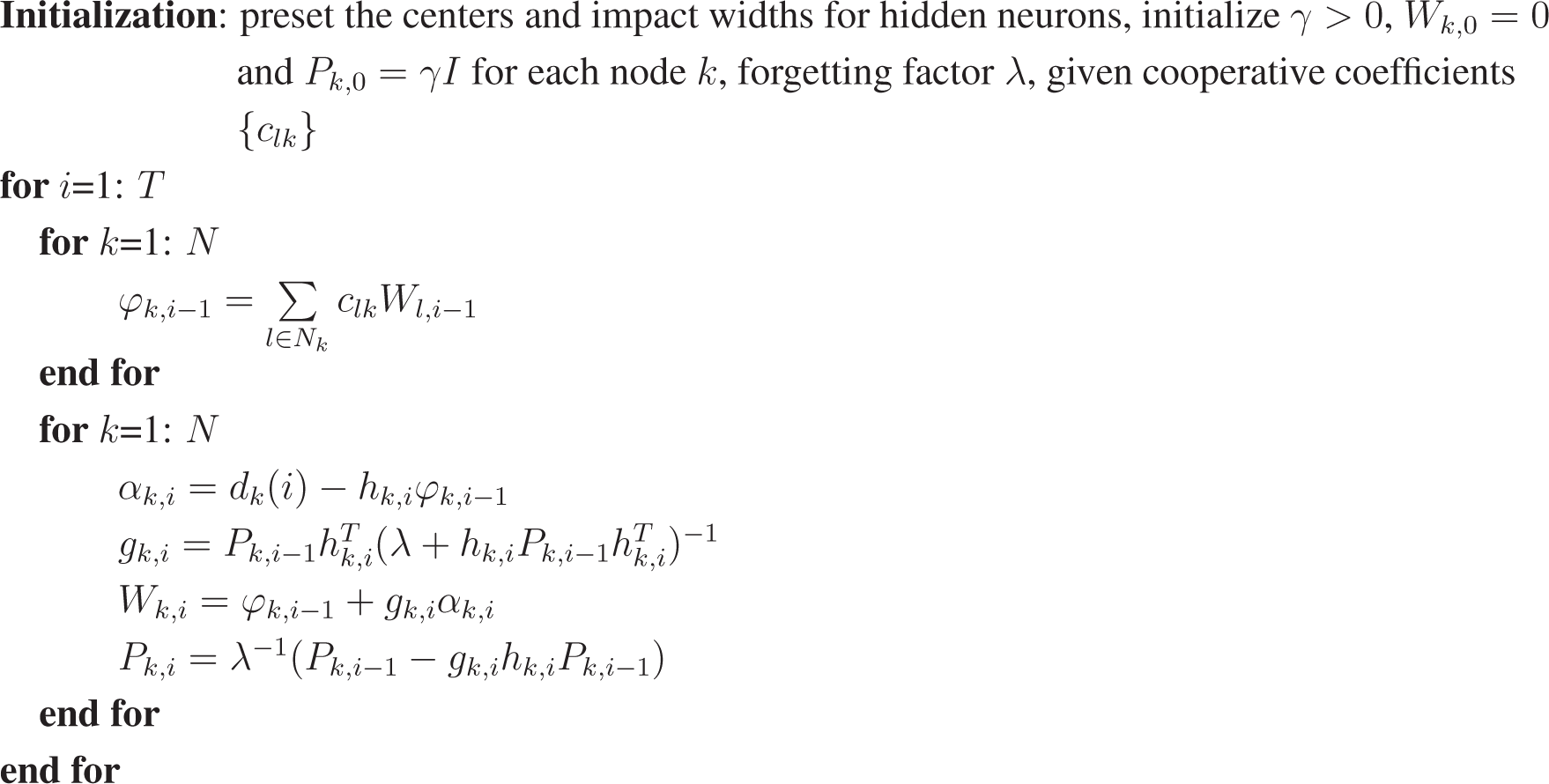
3.2. Distributed ELM-RLS
In this dELM-RLS algorithm, at time i, for each node k, given the measurements collected from Time 1 up to Time i, the local cost function is defined as:
where λ is the forgetting factor and Πi is the regularization matrix. In the RLS algorithm, at each time i, we use the forgetting factor λ to control the amount of the contribution of the previous samples, namely the samples from Time 1 up to Time i–1. In addition, in this paper, we use the exponential regularization matrix λiγ−1I, where γ is a large positive number. We also use the Metropolis rule as the cooperation rule in this dELM-RLS scheme. The regularization item is independent of clk, and
. Thus, we can rewrite Equation (27) as:
Based on the above cost function, for each node k, we can obtain the recursive update formula for the weight matrix by minimizing this local, weighted, regularized cost function, which can be mathematically expressed as:
Similar to the dELM-LMS algorithm, we also define and transmit the intermediate estimate of Wk,i here. Then, replacing the Wk,i in Equation (29) by Equation (14), we can obtain the following minimization of the intermediate estimate:
Equation (30) can be referred to as a least-squares problem. Based on the RLS algorithm, we can obtain the recursive update formula of the intermediate estimate for each node. Since the derivation of the recursive update formula of the intermediate estimate is the same as that presented in the centralized RLS algorithm, we omit the derivation for simplicity in this paper. Finally, we can obtain the two-step recursive update formula for the weight matrix. By performing the “adaptation” step first, we acquire the ATC dELM-RLS algorithm.
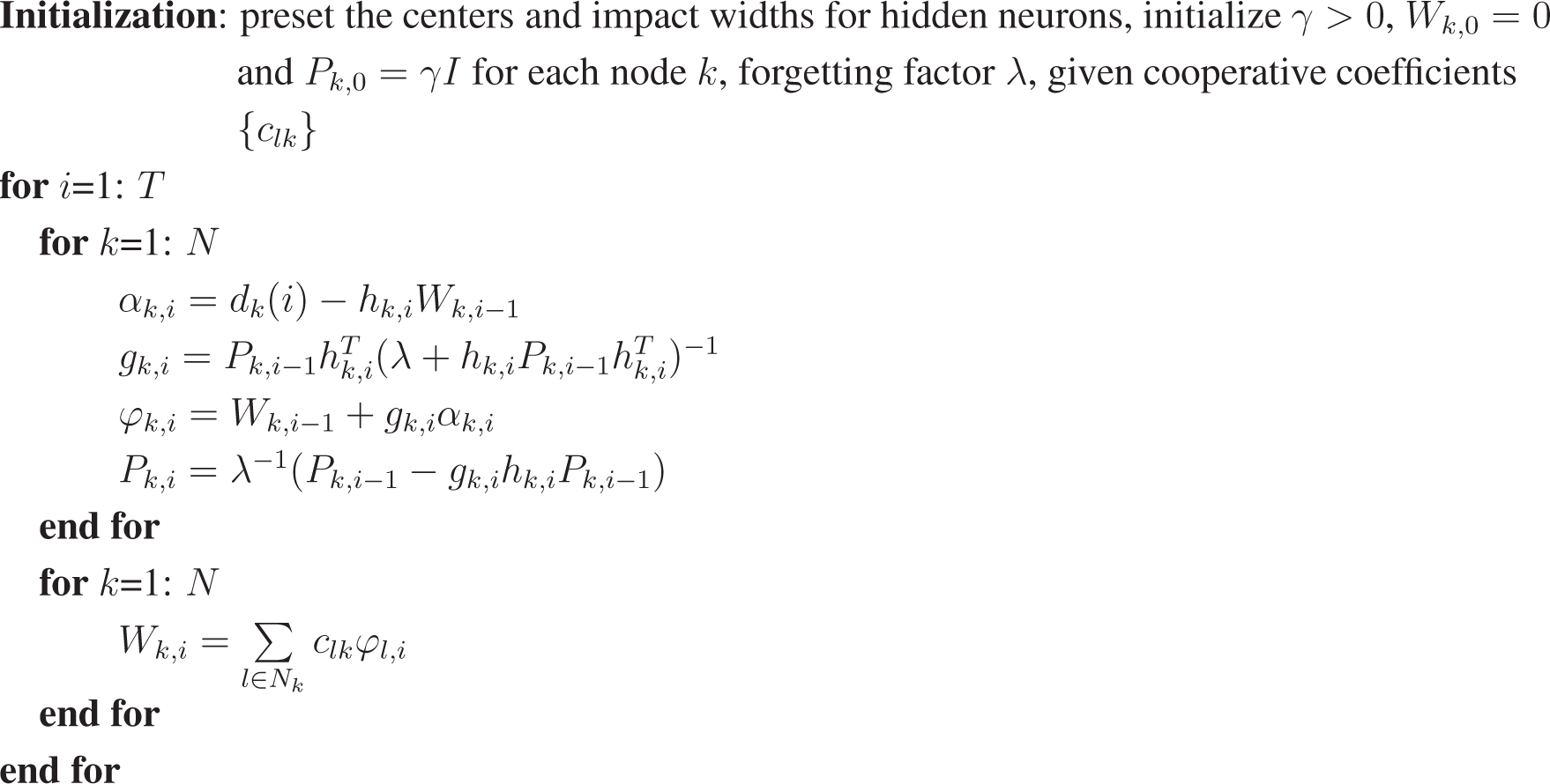
ATC dELM-RLS:
Similarly, we can also obtain the mathematical formula of the CTA dELM-RLS algorithm by just exchanging the order of the “adaptation” step and the “combination” step in each iteration.
CTA dELM-RLS:
In order to clearly present the whole process of the ATC dELM-RLS algorithm and CTA dELM-RLS algorithm, we summarize them in Algorithm 3 and Algorithm 4, respectively.
 |
 |
Based on the idea presented in [26], we can also derive another ATC dELM-RLS algorithm and another CTA dELM-RLS algorithm, which exchange both the original data and the intermediate estimate among the neighbor nodes. Similar to the dELM-LMS case, in the simulation, we find that exchanging the original data does not provide a considerably better performance. Thus, for the purpose of simplicity, we omit the derivation and the simulation results of these dELM-RLS algorithms here.
4. Applications
In this section, we evaluate the performance of distributed ELM algorithms on several benchmark problems [33], which include two regression examples and two classification problems. Specifically, these two regression examples are the fitting of the “Sinc” function and the prediction of the abalone age, and the two classification problems consist of the classification of two “double-moons” and the iris plant. We first present some initial settings for all of these examples. In our examples, the input values of all examples are normalized into [−1,1], while the output values of regression examples are normalized into [0,1].
In the following simulations, to test the performance of the distributed ELM, we compare it with the corresponding non-cooperative scheme in which the intermediate estimates are not shared, namely C = I. In this paper, for each problem, we also present the corresponding centralized solution, which can access all of the training samples. Here, all of the performance measures are averaged over 100 trials. In addition, for the two synthetic data problems, we add Gaussian noise with different signal-to-noise ratios (SNR) to the training sets. Moreover, For all real examples, except for the Landsat satellite image example, in each trial, we randomly select the training samples and the testing samples from the measurements. For the Landsat satellite image example, according to a note provided in [33], we fix the training and testing sets, but change the order of the training set in each trial. For the training data in all of the examples, in each trial, we randomly choose different subsets with the same size for different nodes in the network.
In this paper, to evaluate the performance of the distributed ELM algorithm for the regression problem, we use the standard performance measure, namely, excess mean-square error (EMSE) [1]. As to the classification problem, we use the network misclassification rate (NMCR), which is defined as:
where N is the number of network nodes and MCRk is the misclassification rate of the k-th node in the network. In the first example, we adopt the measure of the transient network EMSE for performance comparison. For the purpose of simplicity, in the other examples, we just present the steady-state NMCR and the steady-state network EMSE for the classification problem and the regression problem, respectively, in the tables. The step size is the same for all nodes. We present the results of the ATC dELM-LMS algorithm and the ATC dELM-RLS algorithm for each example in this paper. As the the results of the CTA-type algorithms are similar to those of the ATC-type algorithms, thus, we omit the results of CTA-type algorithms here. For each problem, we present the comparison of testing results based on all of the algorithms.
We consider a network composed of 10 nodes, which are arranged on a circle. We let each node connect to its nearest one neighbor node on each side and then add some long-range connections with a probability of 0.1. In the RLS-based algorithms, the forgetting factor λ and the large positive number γ are set as 0.995 and 100, respectively. We should notice that the total number of samples for each real example is distinct. However, the number of nodes in the network is the same. Therefore, for different examples, we assign different numbers of samples to each node. Moreover, in this paper, with the given number of samples, the algorithms used in each example all converge to the steady state. Thus, it is rational.
4.1. Regression Problems
4.1.1. Synthetic Data Case: Fitting of the “Sinc” Function
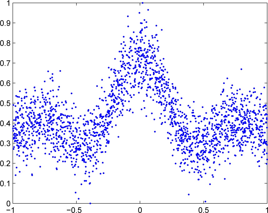
We first evaluate the performance of the distributed ELM algorithms on the fitting of the “Sinc” function problem. The “Sinc” function can be expressed as:
At each trial of this simulation, we uniformly and randomly select 6000 training input data and 2000 testing input data from the interval [−10,10]. Then, we acquire the training output set and the testing output set using the above “Sinc” function with the additive zero-mean Gaussian noise and without noise, respectively. In addition, for each node, at each trial, we randomly select 600 different samples from the training samples. For different nodes, the SNRs are set differently, which vary within [10,20] dB. In order to clearly illustrate this regression problem, we draw 2000 samples from the 6000 training samples and display them in Figure 2. The step size is set as 0.1. We provide 30 hidden neurons for each SLFN in this example.
The learning curves of the dELM-LMS algorithm, the non-cooperative ELM-LMS algorithm and the centralized ELM-LMS algorithm are shown in Figure 3. We see that the dELM-LMS algorithm converges quickly, and the steady-state EMSE of this algorithm is lower than that of the non-cooperative ELM-LMS algorithm and is very close to that of the centralized ELM-LMS algorithm.
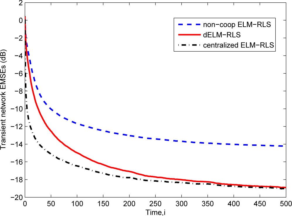
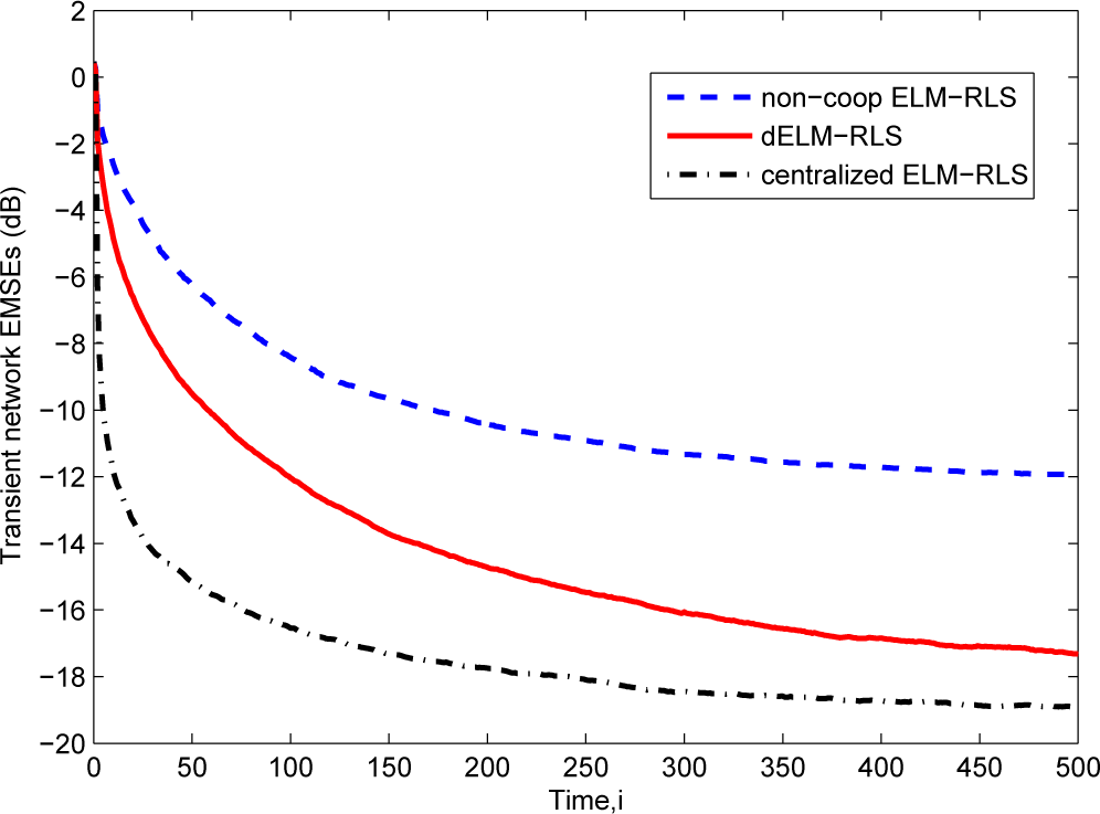
Then, in Figure 4, we give the comparison of the transient network EMSEs of the dELM-RLS algorithm, the non-cooperative ELM-RLS algorithm, and the centralized ELM-RLS algorithm. We see that the steady-state EMSE of the dELM-RLS algorithm is far lower than that of the non-cooperative ELM-RLS algorithm. Although the centralized ELM-RLS converges quickly, the steady-state EMSE of the dELM-RLS is just a little higher than that of the centralized ELM-RLS. In addition, the steady-state network EMSE of the dELM-RLS algorithm is lower than that of the dELM-LMS algorithm, while the computation complexity of the dELM-LMS algorithm is lower than that of the dELM-RLS algorithm. We can get the same observation in the other problems. In real applications, on one hand, we can use the dELM-LMS algorithm when the the computation resource is limited. On the other hand, we can adopt the dELM-RLS algorithm if we demand for high-performance. In conclusion, these simulation results demonstrate the good performance of the distributed ELM algorithms for this “Sinc” function fitting problem.
4.1.2. Real Data Case: Abalone Age Prediction Problem
In biology studies, in order to obtain diverse information, we often need to collect data from different sites. In this case, using a sensor network constituted of several nodes to measure the information and then utilizing local computations based on local communication will make the studies convenient and real time. To simulate the above scenario, we use the developed distributed algorithms for cooperatively predicting the abalone age here. For this example [33], there are 4177 measurements, each of which contains one integer, seven continuous input attributes and one integer output. There are three values for the first integer input attribute, namely male, female and infant. In this paper, We use 0, 1 and 2 to code male, female and infant, respectively. To predict the age of abalone, the eight input attributes are provided.
For this problem, at each trail of simulation, the training dataset and the testing dataset are randomly obtained from the whole abalone database. We present 200 different samples selected from the training dataset for each node at each trail of simulation. Then, we use the remaining 2177 data for testing. The step size is set as 0.1 in this example. We provide 25 hidden neurons for each SLFN in this example.
We first give the comparison of the performance of the dELM-LMS algorithm, the non-cooperative ELM-LMS algorithm and the centralized ELM-LMS algorithm for this abalone age prediction problem. Then, we also present the comparison of the performance of the three ELM-RLS-based algorithms. The results are shown in Table 1. We see that the dELM-LMS algorithm and the dELM-RLS algorithm perform better than the non-cooperative ELM-LMS algorithm and the non-cooperative ELM-RLS algorithm, respectively. In addition, the performance difference between the dELM-LMS algorithm and the centralized ELM-LMS algorithm is very small, and the network EMSE of dELM-RLS algorithm is also very close to that of the centralized ELM-RLS algorithm. These results demonstrate the effectiveness of the distributed ELM algorithms for this abalone age prediction algorithm.
4.2. Classification Problems
4.2.1. Synthetic Data Case: Classification of “Double-Moon”
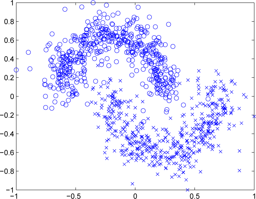
The “Double-Moon” problem is presented here to illustrate the effectiveness of the distributed ELM algorithms for classification. In this problem, as shown in Figure 5, the datasets are shaped as two moons, which are generated by adding noise to two half-circles. We assign the same number of data points to the two moons. The two attributes for this dataset are the coordinates in the horizontal axis and the vertical axis. The aim is to classify the data points into the upper moon and the lower moon using these two attributes.
In this example, at each trail of simulation, we randomly generate 1000 training samples and 1000 testing samples, both with Gaussian zero-mean white noise. In addition, we present 100 different samples drawn from the training dataset for each node at each trail of simulation. The different SNRs varying within [10,20] dB are presented for different nodes. The step size is set as 0.1 here. In this example, the number of hidden neurons for each SLFN is 15. After the network arrives at the steady state, the testing NMCRs of the six algorithms are presented in Table 2. We can see that the performance of the dELM-LMS algorithm and the dELM-RLS algorithm is better than that of the non-cooperative ELM-LMS algorithm and the non-cooperative ELM-RLS algorithm, respectively. In addition, the performance of the dELM-LMS algorithm and the dELM-RLS algorithm approaches that of the centralized ELM-LMS algorithm and the centralized ELM-RLS algorithm, respectively. Thus, for this “Double-Moon” classification problem, the dELM-LMS algorithm and the dELM-RLS algorithm exhibit good performance.
4.2.2. Real data Case: Iris Plant Classification Problem
Botanists often need to consistently record the data of some plants during a considerable long time, which is very difficult, especially in remote regions. We can establish a sensor network covering this region and then use the sensors to record and process the data online. These steps will be useful for the study of plants. In this paper, we consider the famous iris plant classification problem as a simulation of the above scenario. The database of this problem is frequently used in the pattern recognition literature [33]. In this problem, there are four attributes and three classes. Each class corresponds to 50 samples. For these three classes, one of them is linearly separable from the other two classes, while the latter two are not linearly separable. Given the four attributes, namely the sepal length, the sepal width, the petal length and the petal width, our purpose is to classify the iris plants into three classes, which are Iris setosa, Iris versicolor and Iris virginica.
At each trail of the simulation in this example, we randomly select training and testing datasets from the irsdatabase. Twelve different samples randomly picked from the training dataset are presented for each node at each trail of simulation. Then, the remaining 30 samples are used for testing. The step size is set as 0.15 here. In this example, the number of hidden neurons for each SLFN is 30. For this iris plant classification problem, since the number of the samples for each node is very small, to accelerate the convergence speed, firstly, a large initial step size is applied to help the weight matrix converge to the value around the optimal solution fast and, then, a strategy for adaptively adjusting the step size is used to help the algorithm search deeply. Namely, after an iteration, for each node, if
increases, we change the step size by μnew = 0.95μ.
The above six algorithms are also performed for this classification problem. The steady-state NMCRs of these six algorithms are given in Table 3. The steady-state NMCR of the dELM-LMS algorithm is far lower than that of the non-cooperation ELM-LMS algorithm. The performance of the dELM-LMS algorithm approaches that of the centralized ELM-LMS algorithm. As for the three ELM-RLS-based algorithms, the performance difference between the dELM-RLS algorithm and the non-cooperative ELM-RLS algorithm is very obvious. Moreover, the performance of the dELM-RLS algorithm is very close to that of the centralized ELM-RLS algorithm. Thus, for this classification problem, the dELM-LMS algorithm and the dELM-RLS algorithm present good performance.
4.3. Inhomogeneous Data Cases
In some real problems, one node in a network may just obtain a block of the whole measurements, namely the node cannot uniformly and randomly collect data from the whole interval of the measurements, but from a subset of the interval. In these cases, the performance of the non-cooperation algorithms should be poor, and the advantage of the distributed ELM-based algorithms should be more obvious. To simulate these cases, we present the comparison of the performance of the six algorithms for the two synthetic data cases.
4.3.1. Fitting of the “Sinc” Function with Inhomogeneous Data
For this example, we know that the 6000 training input data are selected from the interval [−10,10]. Here, we separate this interval into seven non-overlapping subintervals. At each trial of the simulation, for each node, we randomly select 360 input data from one subinterval and then pick 240 input data from the remaining subintervals. The other settings about the data and the six algorithms are the same as the “Sinc” function fitting problem in Section 4.1. The learning curves of the three ELM-LMS-based algorithms are shown in Figure 6. In this case, we can see that the performance difference between the dELM-LMS algorithm and the non-cooperation ELM-LMS algorithm increases, while the performance difference between the dELM-LMS algorithm and the centralized ELM-LMS algorithm almost remains unchanged.
In Figure 7, the comparison of the transient network EMSEs of the three ELM-RLS-based algorithms are displayed. The performance difference between the dELM-RLS algorithm and the non-cooperation ELM-RLS algorithm become more evident. The performance of the dELM-RLS algorithm is also close to that of the centralized ELM-RLS algorithm.
4.3.2. Classification of the “Double-Moon” with Inhomogeneous Data
For such a situation, we also evaluate the six algorithms for the “Double-Moon” classification problem. In this case, we vertically divide the upper moon and the lower moon from the middle, respectively. For each node, at each trial of the simulation, in each moon, we randomly select 48 data from one of the two halves and then pick two data from the remaining half. Thus, there are 100 data in total for each node. The other settings about the data and the six algorithms are the same as the “Double-Moon” classification problem in Section 4.2. In Table 4, we present the results of the steady-state NMCRs of these six algorithms. We find that the performance difference between the dELM-LMS algorithm and the non-cooperation ELM-LMS algorithm increases for this problem, while the performance difference between the dELM-LMS algorithm and the centralized ELM-LMS algorithm almost remains unchanged. Similarly, the performance difference between the dELM-RLS algorithm and the non-cooperation ELM-RLS algorithm also becomes more obvious for this problem. The performance of the dELM-RLS algorithm approaches that of the centralized ELM-RLS algorithm.
In both examples, the performance of the dELM-LMS algorithm and the non-cooperation ELM-LMS algorithm in the homogeneous data case is better than that of these two algorithms in the inhomogeneous data case, respectively. The performance of the dELM-RLS algorithm and the non-cooperation ELM-RLS algorithm in the homogeneous data case is also better than that of these two algorithms in the inhomogeneous data case, respectively. Given inhomogeneous data, the number of data points in some subinterval may be very small. Thus, the above phenomenon is rational. In addition, as to the real data examples, we also compare the performance of the six algorithms in inhomogeneous data cases. Since the simulation results of the real regression problem and the real classification problem are qualitatively similar to those of the synthetic data regression problem and the synthetic data classification problem, respectively, thus, we omit these results.
5. Conclusion
In this paper, based on the ELM theory, we derived the dELM-LMS algorithm and the dELM-RLS algorithm, which are as simple as the corresponding linear regression algorithms, but applicable to nonlinear learning problems. As we know, due to the limited computational resources in each node, simplicity is quite important. The dELM-LMS algorithm and the dELM-RLS algorithm were then applied to several benchmark problems, including two regression problems and two classification problems. Compared with the non-cooperative ELM-LMS algorithm, the newly-developed dELM-LMS algorithm can converge to a lower steady state. The performance difference between the non-cooperation ELM-RLS algorithm and the dELM-RLS algorithm is also obvious. In addition, the steady-state performance of the dELM-LMS algorithm and the dELM-RLS algorithm is very close to that of the centralized ELM-LMS algorithm and the centralized ELM-RLS algorithm, respectively, for these four benchmark problems. The performance of the dELM-RLS algorithm is better than that of the dELM-LMS algorithm, while the computational complexity of the dELM-LMS algorithm is lower than that of the dELM-RLS algorithm, so we can choose to use different algorithms in different situations. In addition, given inhomogeneous data, the performance difference between the developed distributed algorithms and the corresponding non-cooperation algorithms is more obvious. The performance of the developed distributed algorithms is also close to that of the corresponding centralized algorithms. Overall, the dELM-LMS algorithm and the dELM-RLS algorithm both exhibit good performance for distributed nonlinear learning.
Acknowledgments
This work has been supported by the National Natural Science Foundation of China (Grant Nos. 61171153 and 61101045), the Zhejiang Provincial Natural Science Foundation of China (Grant No. LR12F01001), and the National Program for Special Support of Eminent Professionals.
Author Contributions
Chunguang Li designed the research, Songyan Huang performed the experiment and analyzed the data, both of them wrote the paper. All authors have read and approved the final manuscript.
Conflicts of Interest
The authors declare no conflict of interest.
References
- Cattivelli, F.S.; Lopes, C.G.; Sayed, A.H. Diffusion LMS strategies for distributed estimation. IEEE Trans. Signal Process 2010, 58, 1035–1048. [Google Scholar]
- Dimakis, A.G.; Kar, S.; Moura, J.M.F.M.; Rabbat, G.; Scaglione, A. Gossip algorithms for distributed signal processing. Proc. IEEE 2011, 98, 1847–1864. [Google Scholar]
- Liu, Y.; Li, C.; Tang, W.K.S.; Zhang, Z. Distributed estimation over complex networks. Inf. Sci 2012, 197, 91–104. [Google Scholar]
- Schizas, I.D.; Mateos, G.; Giannakis, G.B. Distributed LMS for consensus-based in-network adaptive processing. IEEE Trans. Signal Process 2009, 57, 2365–2382. [Google Scholar]
- Li, C.; Shen, P.; Liu, Y.; Zhang, Z. Diffusion information theoretic learning for distributed estimation over network. IEEE Trans. Signal Process 2013, 61, 4011–4024. [Google Scholar]
- Lopes, C.G.; Sayed, A.H. Distributed processing over adaptive networks. Proceedings of the Adaptive Sensor Array Processing Workshop, Lexington, MA, USA, 6–7 June 2006; pp. 1–5.
- Cattivelli, F.S.; Sayed, A.H. Analysis of spatial and incermental LMS processing for distribued estimation. IEEE Trans. Signal Process 2011, 59, 1465–1480. [Google Scholar]
- Liu, W.F.; Pokharel, P.P.; Principe, J.C. The kernel least-mean-square algorithm. IEEE Trans. Signal Process 2008, 56, 543–554. [Google Scholar]
- Kivinen, J.; Smola, A.J.; Williamson, R.C. Online learning with kernels. IEEE Trans. Signal Process 2004, 52, 2165–2176. [Google Scholar]
- Censor, Y.; Zenios, S.A. Parallel Optimization: Theory, Algorithms, and Applications; Oxford University Press: New York, NY, USA, 1997. [Google Scholar]
- Predd, J.B.; Kulkarni, S.R.; Poor, H.V. Distributed kernel regression: An algorithm for training collaboratively. Proceedings of the 2006 IEEE Information Theory Workshop, Punta del Este, Uruguay, 13–17 March 2006; pp. 332–336.
- Predd, J.B.; Kulkarni, S.R.; Poor, H.V. A collaborative training algorithm for distributed learning. IEEE Trans. Inf. Theory 2009, 55, 1856–1871. [Google Scholar]
- Perez-Cruz, F.; Kulkarni, S.R. Robust and low complexity distributed kernel least squares learning in sensor networks. IEEE Signal Process. Lett 2010, 17, 355–358. [Google Scholar]
- Chen, S.; Cowan, C.F.N.; Grant, P.M. Orthogonal least squares learning algorithm for radial basis function networks. IEEE Trans. Neural Netw 1991, 2, 302–309. [Google Scholar]
- Huang, G.B.; Zhu, Q.Y.; Siew, C.K. Extreme learning machine: A new learning scheme of feedforward neural networks. Proceedings of International Joint Conference on Neural Networks, Budapest, Hungary, 25–29 July 2004; 2, pp. 985–990.
- Huang, G.B.; Siew, C.K. Extreme learning machine: RBF network case. Proceedings of the 8th International Conference on Control, Automation, Robotics and Vision, Kunming, China, 6–9 December 2004; 2, pp. 1029–1036.
- Liang, N.Y.; Huang, G.B.; Saratchandran, P.; Sundararajan, N. A fast and accurate online sequential learning algorithm for feedforward networks. IEEE Trans. Neural Netw 2006, 17, 1411–1423. [Google Scholar]
- Huang, G.B.; Zhu, Q.Y.; Siew, C.K. Extreme learning machine: Theory and applications. Neurocomputing 2006, 70, 489–501. [Google Scholar]
- Huang, G.B.; Zhou, H.; Ding, X.; Zhang, R. Extreme learning machine for regression and multiclass classification. IEEE Trans. Syst. Man Cybern. B 2012, 42, 513–529. [Google Scholar]
- Rao, C.R.; Mitra, S.K. Generalized Inverse of Matrices and its Applications; Wiley: New York, NY, USA, 1971. [Google Scholar]
- Tu, S.Y.; Sayed, A.H. Diffusion strategies outperform consensus strategies for distributed estiamtion over adaptive networks. IEEE Trans. Signal Process 2012, 60, 6217–6234. [Google Scholar]
- Lopes, C.G.; Sayed, A.H. Diffusion least-mean squares over adaptive networks. Proceedings of the International Conference on Acoustics, Speech, Signal Processing, Honolulu, HI, USA, 15–20 April 2007; 3, pp. 917–920.
- Lopes, C.G.; Sayed, A.H. Diffusion least-mean squares over adaptive networks: Formulation and performance analysis. IEEE Trans. Signal Process 2008, 56, 3122–3136. [Google Scholar]
- Liu, Y.; Li, C.; Zhang, Z. Diffusion sparse least-mean squares over networks. IEEE Trans. Signal Process 2012, 60, 4480–4485. [Google Scholar]
- Cattivelli, F.S.; Lopes, C.G.; Sayed, A.H. A diffusion RLS scheme for distributed estimation over adaptive networks. In. Proceedings of the IEEE 8th Workshop on Signal Processing Advances in Wireless Communications, Helsinki, Finland, 17–20 June 2007; pp. 1–5.
- Cattivelli, F.S.; Lopes, C.G.; Sayed, A.H. Diffusion recursive least-squares for distributed estimation over adaptive networks. IEEE Trans. Signal Process 2008, 56, 1865–1877. [Google Scholar]
- Liu, Z.; Liu, Y.; Li, C. Distributed sparse recursive least-squares over networks. IEEE Trans. Signal Process 2014, 62, 1386–1395. [Google Scholar]
- Xiao, L.; Boyd, S. Fast linear iterations for distributed averaging. Syst. Control Lett 2004, 53, 65–78. [Google Scholar]
- Takahashi, N.; Yamada, I.; Sayed, A.H. Diffusion least-mean squares with adaptive combiners. Proceedings of the International Conference on Acoustics, Speech, Signal Processing, Taipei, Taiwan, 19–24 April 2009; pp. 2845–2848.
- Takahashi, N.; Yamada, I.; Sayed, A.H. Diffusion least-mean squares with adaptive combiners: formulation and performance analysis. IEEE Trans. Signal Process 2010, 58, 4795–4810. [Google Scholar]
- Scherber, D.S.; Papadopoulos, H.C. Locally constructed algorithms for distributed computations in ad hoc networks. Proceedings of the 3rd International Symposium on Information Processing in Sensor Networks, New York, NY, USA, 26–27 April 2004; pp. 11–19.
- Sayed, A.H.; Cattivelli, F. Distributed adaptive learning mechanisms. In Handbook on Array Processing and Sensor Networks; Haykin, S., Ray Liu, K.J., Eds.; Wiley: New York, NY, USA, 2009. [Google Scholar]
- Blake, C.; Merz, C. UCI Repository of Machine Learning Databases. Available Online: http://archive.ics.uci.edu/ml/datasets.html accessed on 12 February 2015.
Figure 1.
Single hidden layer feedforward network.

Figure 2.
Data of the noisy “Sinc” function.

Figure 3.
The transient network EMSEs of the ELM-LMS based algorithms for the “Sinc” function fitting problem.
Figure 3.
The transient network EMSEs of the ELM-LMS based algorithms for the “Sinc” function fitting problem.
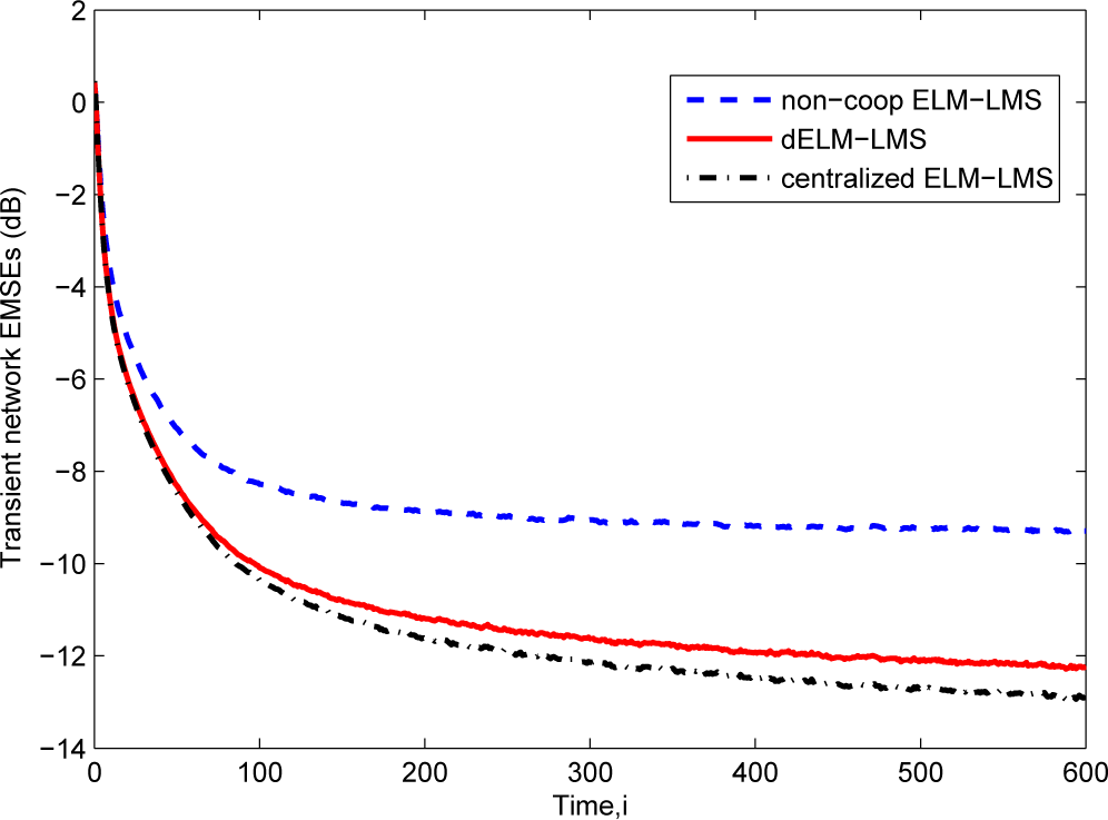
Figure 4.
The transient network excess mean-square errors (EMSEs) of the ELM-RLS based algorithms for the “Sinc” function fitting problem.
Figure 4.
The transient network excess mean-square errors (EMSEs) of the ELM-RLS based algorithms for the “Sinc” function fitting problem.

Figure 5.
Data of the two moons.

Figure 6.
The transient network EMSEs of the ELM-LMS-based algorithms for the “Sinc” function fitting problem with inhomogeneous data.
Figure 6.
The transient network EMSEs of the ELM-LMS-based algorithms for the “Sinc” function fitting problem with inhomogeneous data.
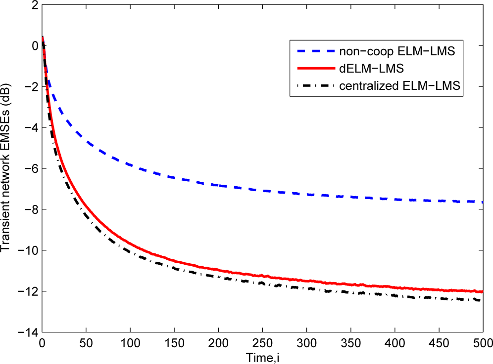
Figure 7.
The transient network EMSEs of the ELM-LMS-based algorithms for the “Sinc” function fitting problem with inhomogeneous data.
Figure 7.
The transient network EMSEs of the ELM-LMS-based algorithms for the “Sinc” function fitting problem with inhomogeneous data.

| Algorithms | steady-state EMSE |
|---|---|
| non-coopELM-LMS | 0.1232 |
| dELM-LMS | 0.1036 |
| centralized ELM-LMS | 0.0989 |
| non-coop ELM-RLS | 0.1079 |
| dELM-RLS | 0.0917 |
| centralized ELM-RLS | 0.0811 |
Table 2.
The steady-state network misclassification rates (NMCRs) of different algorithms for the “Double-Moon” classification problem.
| Algorithms | Steady-state NMCR |
|---|---|
| non-coop ELM-LMS | 8.57% |
| dELM-LMS | 5.46% |
| centralized ELM-LMS | 5.39% |
| non-coop ELM-RLS | 3.35% |
| dELM-RLS | 2.48% |
| centralized ELM-RLS | 2.41% |
| Algorithms | Steady-state NMCR |
|---|---|
| non-coop ELM-LMS | 25.38% |
| dELM-LMS | 10.50% |
| centralized ELM-LMS | 9.87 |
| non-coop ELM-RLS | 11.13% |
| dELM-RLS | 4.24% |
| centralized ELM-RLS | 3.45% |
Table 4.
The steady-state NMCRs of different algorithms for the “Double-Moon” classification problem with inhomogeneous data.
| Algorithms | Steady-state NMCR |
| non-coop ELM-LMS | 13.10% |
| dELM-LMS | 5.51% |
| centralized ELM-LMS | 5.41% |
| non-coop ELM-RLS | 9.74% |
| dELM-RLS | 2.84% |
| centralized ELM-RLS | 2.40% |
© 2015 by the authors; licensee MDPI, Basel, Switzerland This article is an open access article distributed under the terms and conditions of the Creative Commons Attribution license (http://creativecommons.org/licenses/by/4.0/).
Share and Cite
MDPI and ACS Style
Huang, S.; Li, C. Distributed Extreme Learning Machine for Nonlinear Learning over Network. Entropy 2015, 17, 818-840. https://doi.org/10.3390/e17020818
AMA Style
Huang S, Li C. Distributed Extreme Learning Machine for Nonlinear Learning over Network. Entropy. 2015; 17(2):818-840. https://doi.org/10.3390/e17020818
Chicago/Turabian StyleHuang, Songyan, and Chunguang Li. 2015. "Distributed Extreme Learning Machine for Nonlinear Learning over Network" Entropy 17, no. 2: 818-840. https://doi.org/10.3390/e17020818