The Fisher Thermodynamics of Quasi-Probabilities

Abstract

With reference to Lee’s treatment of quasi-probabilities, it is seen that the three phase space quasi-probabilities, known as the P-, Husimi and Wigner ones, plus other intermediate ones, generate a common, single Fisher thermodynamics, along the lines developed by Frieden et al. We explore some facets of such thermodynamics and encounter complementarity between two different kinds of Fisher information.

1. Introduction

This paper revolves around the concept of Fisher’s information measure (FIM), denoted by I, whose utility is continuously growing in the scientific community because of its multiple applications to diverse areas of knowledge [1]. Among its many properties, one of the most important ones is that FIM is a measure of order, as opposed to disorder, best represented by the Gibbs–Boltzmann–Shannon (GBS) entropy S [2]. Information theory (IT), pioneered by Shannon, is able to tell us in precise fashion the information-content of a probability distribution function (PDF) $P\left(i\right)(i=1,\dots ,N)$. In this context, the GBS entropy

$$S=-\sum _{i=1}^{N}P\left(i\right)lnP\left(i\right)$$

(1)

plays a leading role. Jaynes [3] proved that, with Boltzmann’s constant serving as an information unit, one can identify Equation (1) with the thermodynamic entropy, on the the hand, and that statistical mechanics can be reformulated by extremizing S, subject to adequate constraints (the MaxEnt principle [3]). The essence of both thermodynamics and statistical physics is to be found in certain mathematical relations that involve the notions of energy and entropy. These relations provide what one calls the Legendre structure of these two disciplines. Frieden, Plastino, Plastino, and Soffer demonstrated [4] that this Legendre structure remains valid if one changes S by FIM [1].

Frieden and Soffer advanced some time ago [1,5] the idea of a “Fisher temperature” $T_F$ that would play for FIM an identical role as the usual T plays with with regards to the GBS S [3]. This idea was validated later on in a series of papers, by demonstrating that thermodynamics’ Legendre structure is exactly reproduced by using I instead of S [4,6,7,8]. One thus obtains a “Fisher thermodynamics” that is equivalent to the orthodox one. One just replaces S by I [4,6,7,8]. We have thus two conjugate pairs: $(S,T)$ and $(I,T_F)$. Instead of $(1/T)=\text{d}S/\text{d}U$ ($U\equiv$ mean energy) [3], one has $(1/T_F)=\text{d}I/\text{d}U$ [4,6,7,8]. A question naturally emerges what kind of thermometer is to be used for $T_F$? This was answered by Pennini and Plastino in [9], who encountered a simple relation between T and $T_F$.

The above mentioned considerations are mostly concerned with equilibrium statistical mechanics. However, the Fisher information metric has also found applications in Nonequilibrium Statistical Mechanics, see e.g., [10,11,12,13,14,15,16], where one is interested in dynamical properties of systems (e.g., optimal paths, decay modes, etc.).

1.1. Fisher’s Information Measure

Sir Ronald Fisher proposed FIM in 1926 [1,17]. The idea is to study a system specified by a given parameter θ. Let x be a stochastic variable $(\mathbf{\text{x}}\in {\Re }^N)$ and $f_{\theta }\left(\mathbf{\text{x}}\right)$ the probability density (PD) for $\mathbf{\text{x}}$. This PD depends on θ. One now makes a measurement of $\mathbf{\text{x}}$ and wishes on such a basis to estimate θ, obtaining the value $\tilde{\theta }=\tilde{\theta }\left(\mathbf{\text{x}}\right)$. How good is this estimation? The theory of estimation [1] tells us that the best possible estimator $\tilde{\theta }\left(\mathbf{\text{x}}\right)$, if one considers a large number of $\mathbf{\text{x}}$-samples, is characterized by a mean-square error $e^2$ from θ. $e^2$ satisfies a relation that involves FIM: $I{e}^2=1$, where I displays the appearance

$$I=\int \mathrm{d}\mathbf{\text{x}}{f}_{\theta }\left(\mathbf{\text{x}}\right){\left(\frac{\partial ln{f}_{\theta }\left(\mathbf{\text{x}}\right)}{\partial \theta }\right)}^2$$

(2)

This is the optimum estimator, being called the efficient estimator. All possible alternative estimators exhibit a larger mean-square error. The only requisite here is that estimators should always show no bias, that is, they obey $\langle \tilde{\theta }\left(\mathbf{\text{x}}\right)\rangle =\theta$. FIM has a lower bound. No matter which is the parameter, FIM is larger or equal to $1/e^2$. The relationship $I{e}^2\ge 1,$ is the so-called Cramér–Rao bound [1]. A specially important FIM-case should be mentioned. We speak of translation families [1], that is, PDs whose form is invariant against θ-shifts. These distributions are then shift-invariant and $f_{\theta }\left(x\right)=f(x-\theta )$. In this scenario, FIM $I_{si}$ takes the elegant form [1]

$$I_{si}=\int \mathrm{d}\mathbf{\text{x}}f\left(\mathbf{\text{x}}\right){\left(\frac{\partial lnf\left(\mathbf{\text{x}}\right)}{\partial \mathbf{\text{x}}}\right)}^2$$

(3)

FIM is additive [1]: Let $\mathbf{\text{x}}\mathrm{and}\mathbf{\text{p}}$ be independent variables. Then $I_{si}(\mathbf{\text{x}}+\mathbf{\text{p}})=I_{si}\left(\mathbf{\text{x}}\right)+I_{si}\left(\mathbf{\text{p}}\right)$. Accordingly, in estimating the location of a phase space point $(\mathbf{\text{x}},\mathbf{\text{p}})$, one encounters a shift-invariance scenario.

In this work, we will appeal to two versions of the Fisher information: (1) $I_{si}$ and (2) the one in which the parameter θ equals the inverse temperature β.

1.2. Quasi-Probabilities

It is well known that one writes the density operator in diagonal fashion ($P-$representation) in terms of coherent states $|\alpha \rangle$ as [18,19]

$$\widehat{\rho }=\int \frac{d^2\alpha }{\pi }P\left(\alpha \right)|\alpha \rangle \langle \alpha |$$

(4)

$P\left(\alpha \right)$ is referred to as a quasi-probability since it can adopt negative values because of normalization [18].

$$\mathrm{Tr}\widehat{\rho }=\int \frac{{\text{d}}^2\alpha }{\pi }P\left(\alpha \right)=1$$

(5)

Usually, $|\alpha \rangle$ are harmonic oscillator coherent states obeying $\widehat{a}|\alpha \rangle =\alpha |\alpha \rangle$ [18], with complex with complex α and $\langle \alpha |\alpha \rangle =1$, so that [18].

$$\int \frac{{\text{d}}^2\alpha }{\pi }|\alpha \rangle \langle \alpha |=1$$

(6)

From Equation (4), it is possible to generate a vast list of alternative quantum distributions in phase space, such as, for example, the so-called Q-function [20], and of the celebrated Wigner’s W-function [21,22]. For an arbitrary density operator, the connection between Q- and P- functions, through the following convolution transformation, is given by [22]

$$Q\left(z\right)=\int \frac{{\text{d}}^2\alpha }{\pi }P\left(\alpha \right)e^{{-|\alpha -z|}^2}$$

(7)

1.3. Our Goal

Our purpose in this paper is to investigate the Fisher thermodynamics associated with quasi-probabilities, i.e., to translate Fisher-thermodynamics’s ideas into phase space parlance. It will be seen that interesting insights are provided by such a translation.

The paper is organized as follows. The first three Sections expound preliminary materials. In Section 2, we revisit some key ideas developed in [4,9] but reexpressing them in a phase space language. In Section 3, we recapitulate the quasi-probabilities treatment of Lee [23], and finally, in Section 4, we discuss the effective temperature approach for quasi-probabilities developed in [24]. The subsequent three Sections convey our new materials. Section 5 relates Fisher’s measure to the effective temperature of [24]. Section 6 discusses that special kind of Fisher information indicator (cf. Equation (2)) whose parameter θ is the inverse effective temperature, and Section 7 introduces the important notion of Fisher complementarity. Conclusions are drawn in Section 8.

2. Fisher Information’s Relations in Phase Space

We review in this Section some key ideas developed in [4,9], but reexpressing them in a phase space language. The MaxEnt classical density that describes a system at equilibrium is [3]

$$\rho \left(\alpha \right)=\frac{1}{\mathcal{Z}}{e}^{-{\sum }_{i=1}^M{\chi }_i{A}_i\left(\alpha \right)}$$

(8)

where the complex quantity α is linear superposition of phase space variables x-p. The partition function $\mathcal{Z}$ has the form $\mathcal{Z}\left({\chi }_i\right)=\int ({\text{d}}^2\alpha /\pi )exp(-{\sum }_{i=1}^M{\chi }_i{A}_i\left(\alpha \right)),$ $i=1,\dots ,M$ [3], with ${\text{d}}^2\alpha =\text{d}x\text{d}p/2\pi \hslash$. The ${\chi }_i$ are MaxEnt Lagrangian multipliers associated to $M-$observables $A_i\left(\alpha \right)$, with the

$$\langle A_i\rangle =\int \frac{{\text{d}}^2\alpha }{\pi }\rho \left(\alpha \right)A_i\left(\alpha \right)$$

(9)

constituting our prior information. Recourse to the MaxEnt prescriptions yields the ${\chi }_i$ of Equation (8).

Mandelbrot suggests [9,25,26,27] that we link these ${\chi }_i$ to parameters to be estimated via Fisher-manipulations (cf. Equation (2)) using an FIM depending on ρ that is cast as a sum of M-terms $T_i$ (one for each ${\chi }_i$ (cf. Equation (7)) (see also [9])

$$I=\sum _{i=1}^M{\Gamma }_i〈{\left(\frac{\partial ln\rho }{\partial {\chi }_i}\right)}^2〉=\sum _{i=1}^M{\Gamma }_i〈{\left(A_i-\langle A_i\rangle \right)}^2〉$$

(10)

We see that I is associated to fluctuations of the observables [25,26,27,28]. In addition, ${\Gamma }_i$ are suitable constants, useful to render a dimensionless Fisher measure I [9]. Our statistical fluctuations obey the relation [25,26,27,28]

$$〈{\left(A_i-\langle A_i\rangle \right)}^2〉=-\frac{\partial \langle A_i\rangle }{\partial {\chi }_i}$$

(11)

so that FIM turns out to be

$$I=-\sum _{i=1}^M{\Gamma }_i\frac{\partial \langle A_i\rangle }{\partial {\chi }_i}$$

(12)

As stated above, thermodynamics’ Legendre structure arises from extremizing I with adequate constraints [4,6,7,8]. We use the same $\langle A_i\rangle$ with different Lagrange multipliers. This procedure is the counterpart of Shannon’s MaxEnt procedure. The new Fisher multipliers are, say, ${\gamma }_i$. One now appeals to the well known thermodynamic relation associating (i) the information measure; (ii) the Lagrange multipliers (Fisher’s here); and (iii) expectation values [4]

$${\gamma }_i=\frac{\partial I}{\partial \langle A_i\rangle }$$

(13)

Inserting this into Equation (12), we can cast Fisher’s ${\gamma }_i$ in terms of Shannon’s ones (${\chi }_j$’s),

$${\gamma }_i=-\sum _{j=1}^M{\Gamma }_j\frac{\partial }{\partial \langle A_i\rangle }\frac{\partial \langle A_j\rangle }{\partial {\chi }_j}$$

(14)

a relation which could be used to determine them.

Let us assume that the thermal equilibrium Boltzmann-Gibbs probability distribution is ($\beta =1/kT$), for any system of energy E

$$\rho =exp(-\beta E)/\mathcal{Z}$$

(15)

and set $\Gamma =1/k_B{T}_0$. We have introduced an arbitrary, fixed reference temperature $T_0$. The (dimensionless) canonical ensemble FIM Equation (12) becomes now

$$I=-\frac{1}{k^2{T}_0^2}\frac{\partial \langle E\rangle }{\partial \beta }$$

(16)

As stipulated in [9], if we assume that the system obeys the energy’s equipartition theorem in a phase space of two degrees of freedom, i.e., using Equation (9)

$$U=\langle E\rangle ={\beta }^{-1};\frac{\partial E}{\partial \beta }=-{\beta }^{-2}=-{\langle E\rangle }^2$$

(17)

The Fisher multiplier is, according to Equation (14), and introducing at this point the Fisher temperature $T_F$,

$$\gamma \equiv \frac{1}{k{T}_F}=-\frac{1}{k^2{T}_0^2}\frac{\partial }{\partial \langle E\rangle }\frac{\partial \langle E\rangle }{\partial \beta }=\frac{2}{k^2{T}_0^2\beta }=\frac{2kT}{k^2{T}_0^2}$$

(18)

From this fact, we get the relationship between the Fisher temperature and the ordinary, Shannon’s one T

$$T_F=\frac{T_0^2}{2T}$$

(19)

and emphasize that, if I grows, then S diminishes, and vice versa [1]. As a consequence, the very thermometer that indicates T values can also be employed to ascertain $T_F$, relabelling its scale.

3. Lee’s Quasi-Probability Distributions R

Consider a continuous parameter τ. With the purpose to connect all phase space distributions (quasi probabilities), Ching Tsung Lee introduces it in the transformation (convolution) P-Q, and defines a generalized distribution function as follows [23]

$$R(z,\tau )=\frac{1}{\tau }\int \frac{{\text{d}}^2\alpha }{\pi }P\left(\alpha \right)exp\left(-\frac{1}{\tau }{|z-\alpha |}^2\right)$$

(20)

For $\tau =0,$ $1/2$, and 1, this R function becomes the $P,$ W and Q ones, respectively. We see that R is a continuous interpolation between P and Q [23]. Thus, the formalism is restricted to τ-values between 0 to 1.

In particular, for a thermal quantum state of the harmonic oscillator at the temperature T ($\beta =1/kT$), the P-function is ($\widehat{n}$ is the phonon-number operator)

$$P\left(\alpha \right)=\frac{1}{\langle \widehat{n}\rangle }exp\left(-\frac{{\left|\alpha \right|}^2}{\langle \widehat{n}\rangle }\right)$$

(21)

while the mean phonon-number is [18]

$$\langle \widehat{n}\rangle =\frac{e^{-\beta \hslash \omega }}{1-e^{-\beta \hslash \omega }}$$

(22)

which obviously depends on the temperature T.

Introducing Equation (21) into Equation (20) and integrating on the variable α with the help of the integral

$$\int \frac{{\text{d}}^2\alpha }{\pi }{e}^{-{\gamma \left|\alpha \right|}^2}{e}^{z{\alpha }^{*}+z^{*}\alpha }={\gamma }^{-1}{e}^{{\gamma }^{-1}{\left|z\right|}^2}$$

(23)

we can get the analytical thermal R-function. With a simple calculation, we discover here that one can cast the quantum HO’s R as

$$R(z,\tau )=\frac{1}{\tau +\langle \widehat{n}\rangle }exp\left(-\frac{{\left|z\right|}^2}{\tau +\langle \widehat{n}\rangle }\right)$$

(24)

which depends on the temperature via the above definition of $\langle \widehat{n}\rangle$ given by Equation (22). We emphasize some specific cases such as

$$\begin{array}{ccc}\hfill R(z,0)={\gamma }_P{e}^{-{\gamma }_P{\left|\alpha \right|}^2},{\gamma }_P& =& \frac{1}{\langle \widehat{n}\rangle }=e^{\beta \hslash \omega }-1\left(P-\mathrm{function}\right)\hfill \end{array}$$

(25)

$$\begin{array}{ccc}\hfill R(z,1)={\gamma }_Q{e}^{-{\gamma }_Q{\left|\alpha \right|}^2}{\gamma }_Q& =& \frac{1}{1+\langle \widehat{n}\rangle }=1-e^{-\beta \hslash \omega }\left(Q-\mathrm{function}\right)\hfill \end{array}$$

(26)

$$\begin{array}{ccc}\hfill R(z,1/2)={\gamma }_W{e}^{-{\gamma }_W{\left|\alpha \right|}^2}{\gamma }_W& =& \frac{1}{1/2+\langle \widehat{n}\rangle }=2tanh(\beta \hslash \omega /2)\left(W-\mathrm{function}\right)\hfill \end{array}$$

(27)

We note that the P(Q) representation corresponds to a normal (antinormal) ordering of the creation and destruction operators. However, in the limit of high temperatures, $T\gg \hslash \omega /k$, we can ignore this ordering of operators, which it will then not be considered in the forthcoming Section. In this limit, all effects are classical.

4. Review of the Effective Temperature Treatment of Quasi-Probabilities

To end our recapitulation process, we review here now ideas of [24] that will be later generalized à la Fisher. Let us define the classical expectation value of the arbitrary function $\mathcal{A}(x,p)$ as

$$\langle \mathcal{A}\rangle =\int \frac{{\text{d}}^2\alpha }{\pi }R(\alpha ,\tau )\mathcal{A}\left(\alpha \right)$$

(28)

where we have considered the thermal $R(\alpha ,\tau )$ given by Equation (24) as the statistical weight function. The idea to be advanced at this stage is the following. We are dealing with quasi-probabilities R for canonical thermal states of a quantum harmonic oscillator (HO) distribution (of temperature T), but we consider now a special HO, namely, a classical one at the temperature $T^{*}$. Thus, the associated canonical ensemble assumes interaction with a reservoir of hat at the temperature $T^{*}$. The pertinent effective, classical HO-Hamiltonian reads [24]

$$\mathcal{H}(x,p)={\hslash \omega \left|\alpha \right|}^2$$

(29)

where x and p are phase space variables, ${\left|\alpha \right|}^2=x^2/4{\sigma }_x^2+p^2/{\sigma }_p^2$, and ${\sigma }_x^2=\hslash /2m\omega$ and ${\sigma }_p^2=\hslash m\omega /2$ [3].

Let us discuss in some more detail the concept of effective temperature [24] with reference to the mean value $U^{*}$ of the effective Hamiltonian for a given free parameter $\langle n\rangle$ that mimics the mean phonon number $\langle \widehat{n}\rangle$, defined as

$$\langle n\rangle =\frac{e^{-\beta \hslash \omega }}{1-e^{-\beta \hslash \omega }}$$

(30)

so that

$$U^{*}=\hslash \omega \int \frac{{\text{d}}^2\alpha }{\pi }R(\alpha ,\tau ){\left|\alpha \right|}^2=\hslash \omega (\tau +\langle n\rangle )$$

(31)

Introducing Boltzmann’s constant k, our effective temperature $T^{*}$, via equipartition (two degrees of freedom), becomes

$$T^{*}=\frac{U^{*}}{k}$$

(32)

that is, we reiterate that $U^{*}$ is the classical mean energy of a harmonic oscillator at the effective temperature $T^{*}$ and mean phonon number $<n>$

$$U^{*}=k{T}^{*}$$

(33)

with

$$T^{*}=\frac{\hslash \omega }{k}(\tau +\langle n\rangle )$$

(34)

contributing with $k{T}^{*}/2$ for each of the two pertinent degrees of freedom. The concept of effective temperature $T^{*}$ is fundamental for us here because it absorbs τ. The treatment in terms of $T^{*}$ accommodates all possible τ values into a single expression. The condition $\tau +\langle n\rangle >0$ ensures positivity of $T^{*}$. This entails $\tau >0$. Taking into account the definition Equation (31), we recast Equation (24) in the following manner

$$R(z,\tau )={\beta }^{*}\hslash \omega exp\left(-{\beta }^{*}\hslash \omega {\left|z\right|}^2\right)$$

(35)

that is the thermal equilibrium Boltzmann–Gibbs probability distribution at the equilibrium temperature $T^{*}$, with ${\beta }^{*}=1/k{T}^{*}$. This is equivalent to the probability distribution of a classical harmonic oscillator in a canonical ensemble contained in a volume V whose energy is given by Equation (31), with ${\beta }^{*}$ playing the role of a Lagrange multiplier. In view of the definition Equation (24), we immediately obtain the partition function $Z^{*}$ whose appearance is

$$Z^{*}=\int \frac{{\text{d}}^2\alpha }{\pi }exp(-{\beta }^{*}{\hslash \omega \left|\alpha \right|}^2)=\tau +\langle n\rangle$$

(36)

Additionally, the thermodynamic entropy S is

$$S=k(1-ln(\tau +\langle n\rangle )$$

(37)

that from Equation (33), it can be rewritten as a function of $T^{*}$as

$$\frac{S}{k}=1+ln\left(\frac{k{T}^{*}}{\hslash \omega }\right)$$

(38)

Combining Equation (33) with the thermodynamic entropy Equation (37), it is easy to verify that

$$T^{*}={\left(\frac{\partial U^{*}}{\partial S}\right)}_V$$

(39)

where we have considered the volume V to be constant. The effective Helmholtz free energy is given by

$$A^{*}=U^{*}-T^{*}S=k{T}^{*}ln\left(\frac{\hslash \omega }{k{T}^{*}}\right).$$

(40)

In addition, according to Equations (31), (36) and (37), we find

$$\frac{S}{k}=ln{Z}^{*}+{\beta }^{*}{U}^{*}$$

(41)

Thus, one reobtains, for any Lee quasi-probability distribution, all the thermal results pertaining to a classical HO at the temperature $T^{*}$. Let us insist: the above results are valid for any given Lee quasi-probability distribution.

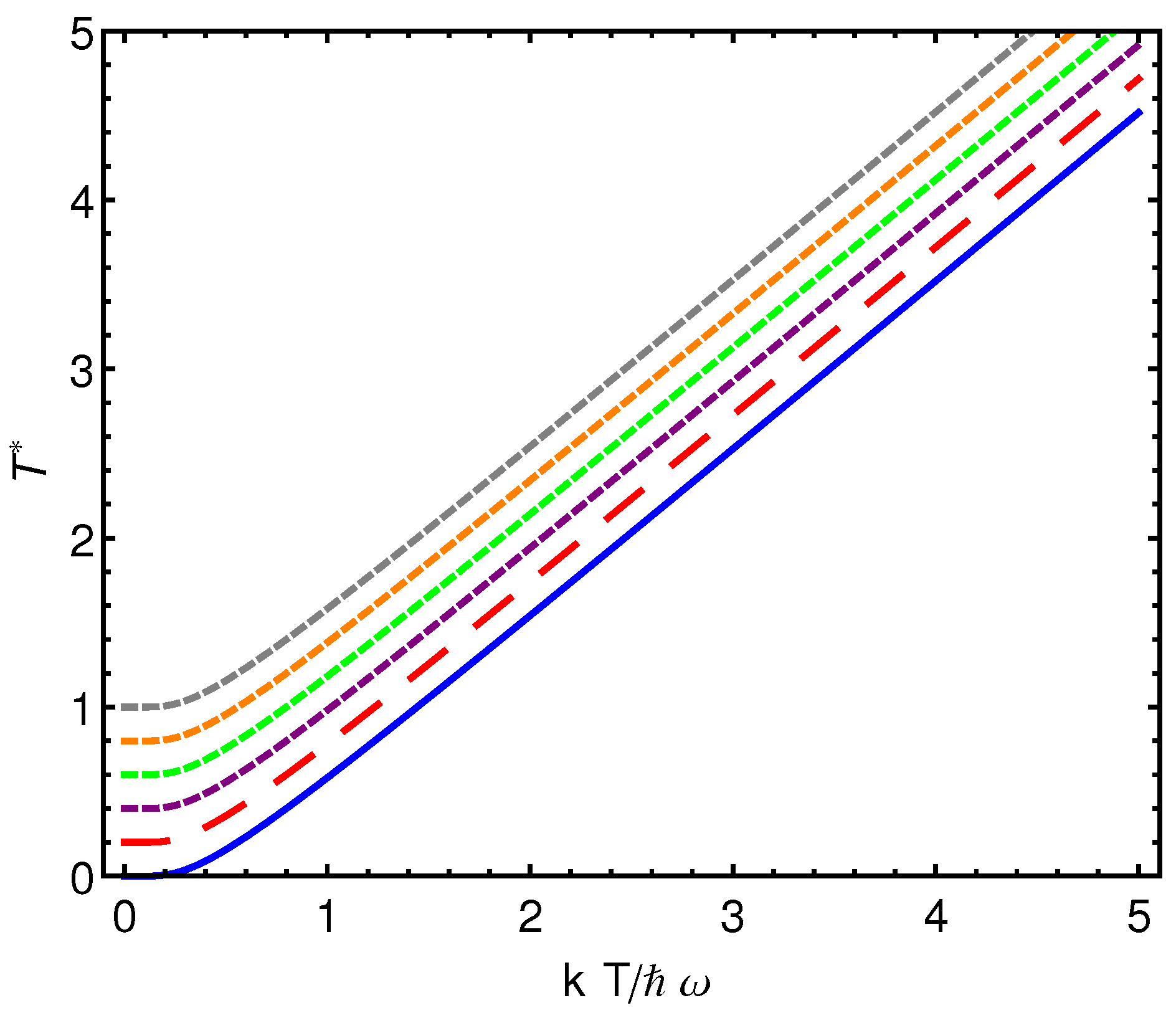
In Figure 1, we show the comportment of $T^{*}$ vs. T for several values of τ. We remark that, save for a small T-zone near the origin, the τ-curves are of a linear character, so that $T^{*}$ depends linearly on T and can be measured with the same thermometer, with a trivial relabelling. This small T-zone near the origin is not relevant for our present classical (or semiclassical) regimes, since the concomitant T∼0 scenario can not be properly described by such regimes.

Figure 1. $T^{*}$ versus $kT/\hslash \omega$ for τ = 0, 0.2, 0.4, 0.6, 0.8, 1 (upwards).

Figure 1. $T^{*}$ versus $kT/\hslash \omega$ for τ = 0, 0.2, 0.4, 0.6, 0.8, 1 (upwards).

5. Fisher’s Measure and Effective Temperature

We begin here developing the contributions of this work. Our shift-invariant Fisher information $I_{si}$ in phase space, adapted to the preceding considerations, reads

$$I_{si}=\frac{1}{4}\int \frac{{\text{d}}^2\alpha }{\pi }R(\alpha ,\tau ){\left(\frac{\partial lnR(\alpha ,\tau )}{\partial \left|\alpha \right|}\right)}^2$$

(42)

so that, dealing with this integral, we are led to the result

$$I_{si}=\frac{1}{\tau +\langle n\rangle }$$

(43)

a dimensionless quantity.

As in the preceding Section, we wish to accommodate all possible τ values into a single reference frame. For that, we invoke the effective temperature $T^{*}$ of the preceding Section and cast I in terms of $T^{*}$ as

$$I_{si}=\frac{\hslash \omega }{k{T}^{*}}={\beta }^{*}\hslash \omega$$

(44)

and, we are led, from Equations (37) and (44), to the universal relationship

$$\frac{S}{k}=1-ln{I}_{si}$$

(45)

or

$$e^{S/k}=\frac{e}{I_{si}}$$

(46)

entailing that this relation is universally valid for all quasi probability distributions for all $0\le \tau \le 1$. This is a very important result. For quasi probabilities, there exists an analytical relationship between S and $I_{si}$, that, as far as we know, is the first to be encountered in the Literature.

6. Another Kind of Fisher Information

Up to now, we have dealt only with the so-called shift invariant FIM $I_{\tau }$. In this subsection, we appeal to another FIM (cf. Equation (2)), one for which the pertinent parameter is the effective inverse temperature ${\beta }^{*}$. Note that in Ref. [29], its authors use the same FIM, but that their parameter is, instead, β. We consider a system at thermal equilibrium described by the Gaussian distribution $R(\alpha ,\tau )$ given by Equation (35). For this Gaussian distribution, we define the ${\beta }^{*}$-Fisher measure as [29]

$$I_{{\beta }^{*}}=\int \frac{{\text{d}}^2\alpha }{\pi }R(\alpha ,\tau ){\left(\frac{\partial lnR(\alpha ,\tau )}{\partial {\beta }^{*}}\right)}^2$$

(47)

so that by integrating over phase space, we immediately get

$$I_{{\beta }^{*}}=\frac{1}{{{\beta }^{*}}^2}.$$

(48)

On the other hand, from Equation (33) and definition of ${\beta }^{*}$ we have

$$\frac{\partial U^{*}}{\partial {\beta }^{*}}=-\frac{1}{{{\beta }^{*}}^2}$$

(49)

so that, replacing this into Equation (48), one obtains the important relationship

$$I_{{\beta }^{*}}=-\frac{\partial U^{*}}{\partial {\beta }^{*}}$$

(50)

which casts $I_{{\beta }^{*}}$ as a first derivative of the mean energy. The dimensionless expression for this FIM is, according to the concepts expounded in Section 2 and appealing to the reference $T_0$,

$$I_{{\beta }^{*}}^{{}^{\prime }}=\frac{I_{{\beta }^{*}}}{k^2{T}_0^2}=-\frac{1}{k^2{T_0}^2}\frac{\partial U^{*}}{\partial {\beta }^{*}}.$$

(51)

The pertinent FIM multiplier is, looking back at Section 2,

$$\gamma =\frac{1}{k{T}_F}=-\frac{1}{k^2{T_0}^2}\frac{\partial }{\partial U^{*}}\frac{\partial U^{*}}{\partial {\beta }^{*}}=\frac{2}{k^2{T_0}^2{\beta }^{*}}$$

(52)

leading to the relationship

$$T_F=\frac{{T_0}^2}{2T^{*}}=\frac{{T_0}^2}{2\hslash \omega (\tau +\langle n\rangle )}.$$

(53)

We see that the relationship between $T_F$ and $T^{*}$ is akin to that between $T_F$ and T.

7. Fisher Complementarity

We appeal now to the quantum, Bohr’s notion of complementarity [30,31,32]. According to it, some objects display complementary properties that one can not simultaneously measure with accuracy. The more precisely one property is ascertained, the more uncertain the determination of the complementary property becomes. Heisenberg’s uncertainty relation is the paramount instantiation. A long time has elapsed since its original formulation. However, an important debate is still going on regarding both its interpretation and its precise definition in several contexts [33,34,35,36]. We encounter below a classical instantiation of the principle, a Fisher one.

From Equations (44) and (48), we immediately find

$$I_{{\beta }^{*}}=\frac{{\hslash }^2{\omega }^2}{{\hslash }^2{\omega }^2{{\beta }^{*}}^2}=\frac{{\hslash }^2{\omega }^2}{I_{si}^2}.$$

(54)

since $I_{si}$ is dimensionless, $I_{\beta }$ has units of energy squared.

Once again, we find an analytical expression relating our two FIMs.

By taking logarithms and considering the relation Equation (45) between S and $I_{si}$, after some algebra we obtain a relation between S and $I_{{\beta }^{*}}$

$$I_{{\beta }^{*}}={\hslash }^2{\omega }^2{e}^{2(S/k-1)}$$

(55)

or

$$\frac{S}{k}=\frac{1}{2}ln\left(\frac{e{I}_{{\beta }^{*}}}{\hslash \omega }\right)$$

(56)

which links analytically the new FIM to S. In addition, from Equation (54), we encounter complementarity, i.e., at a sort on uncertainty relation

$$\sqrt{I_{{\beta }^{*}}}{I}_{si}=\hslash \omega$$

(57)

or in view of Equation (51)

$$\sqrt{I_{{\beta }^{*}}^{{}^{\prime }}}{I}_{si}=\frac{\hslash \omega }{k{T}_0}=\mathrm{constant}$$

(58)

which improves upon a similar relationship encountered in [29], where, however, (i) on the right hand side, there is not a constant, but it depends on the temperature (i.e., on the reservoir and not on the system), and thus no proper uncertainty arises and (ii) one deals there with $I_{\beta }$ and not with $I_{{\beta }^{*}}$. Note that for $\hslash \omega$ we have a well known physical meaning: the energetic distance between HO-levels.

$I_{{\beta }^{*}}$ coveys information regarding the effective temperature, while $I_{si}$ refers to information about phase space localization. We discover here that these two types of information are complementary. If one becomes larger, the other diminishes.

8. Conclusions

In this paper, for quadratic Hamiltonians, with reference to Lee’s quasi-probability phase space distributions, we have:

• Reexpressed the Lee distribution $R(z,\tau )$ in terms of the temperature T expressed via the parameter $\langle n\rangle$ (cf. Equation (30)).
• Linked the concept of phase space effective temperature, advanced in [24] to Fisher-quantities. We discovered that, for Lee’s quasi-probabilities [23], there exists an analytic expression linking the phase space entropy S to its shift-invariant Fisher counterpart $I_{si}$. The existence of such a link was not known before, as far as we know.
• Encountered, by analysis of the special kind of Fisher-measure $I_{{\beta }^{*}}$, whose parameter is the inverse effective Fisher temperature, that the Fisher temperature $T_F$ of reference [9] behaves like the inverse of the effective temperature of reference [24].
• Discovered a Bohr’s complementarity between $I_{{\beta }^{*}}$ and the shift-invariant measure $I_{si}$, showing that the associated celebrated Principle applies to some Information Theory entities.

References

- Frieden, B.R. Physics from Fisher Information; Cambridge University Press: Cambridge, UK, 1998. [Google Scholar]
- Frieden, B.R.; Hawkins, R.J. Quantifying system order for full and partial coarse graining. Phys. Rev. E 2010, 82, 066117. [Google Scholar] [CrossRef] [PubMed]
- Katz, A. Principles of Statistical Mechanics; W.H. Freeman and Company: San Francisco, CA, USA, 1967. [Google Scholar]
- Frieden, B.R.; Plastino, A.; Plastino, A.R.; Soffer, H. Fisher-based thermodynamics: Its Legendre transforma and concavity properties. Phys. Rev. E 1999, 60, 48–53. [Google Scholar] [CrossRef]
- Frieden, B.R.; Soffer, B.H. Lafrangians of physics and the game of Fisher-information transfer. Phys. Rev. E 1995, 52. [Google Scholar] [CrossRef]
- Frieden, B.R.; Plastino, A.; Plastino, A.R.; Soffer, B. A Schrödinger link between non-equilibrium thermodynamics and Fisher information. 2002; arXiv:cond-mat/0206107. [Google Scholar]
- Frieden, B.R.; Plastino, A.; Plastino, A.R.; Soffer, B.H. Non-equilibrium thermodynamics and Fisher information: An illustrative example. Phys. Lett. A 2002, 304, 73–78. [Google Scholar] [CrossRef]
- Flego, S.P.; Frieden, B.R.; Plastino, A.; Plastino, A.R.; Soffer, B.H. Nonequilibrium thermodynamics and Fisher information: Sound wave propagation in a dilute gas. Phys. Rev. E 2003, 68, 016105. [Google Scholar] [CrossRef] [PubMed]
- Pennini, F.; Pastino, A. Reciprocity relations between ordinary temperature and the Frieden-Soffer Fisher temperature. Phy. Rev. E 2005, 71, 047102. [Google Scholar] [CrossRef] [PubMed]
- Zanardi, P.; Giorda, P.; Cozzini, M. Information-theoretic differential geometry of quantum phase transitions. Phys. Rev. Lett. 2007, 99, 100603. [Google Scholar] [CrossRef] [PubMed]
- Ercolessi, E.; Schiavina, M. Geometry of mixed states for a q-bit and the quantum Fisher information tensor. J. Phys. A Math. Theor. 2012, 45, 365303. [Google Scholar] [CrossRef]
- Polettini, M. Nonequilibrium thermodynamics as a gauge theory. Europhys. Lett. 2012, 97, 30003. [Google Scholar] [CrossRef]
- Polettini, M.; Esposito, M. Nonconvexity of the relative entropy for Markov dynamics: A Fisher information approach. Phys. Rev. E. 2013, 88, 012112. [Google Scholar] [CrossRef] [PubMed]
- Polettini, M. Fisher information of Markovian decay modes. Europhys. J. B 2014, 87. [Google Scholar] [CrossRef]
- Nicholson, S.B. The Geometry of Chance: On the Theory of Non-Equilibrium Statistical Mechanics. Ph.D. Thesis, University of Sheffield, Sheffield, UK, 2015. [Google Scholar]
- Crooks, G.E. Measuring thermodynamic length. Phys. Rev. Lett. 2007, 99, 100602. [Google Scholar] [CrossRef] [PubMed]
- Frieden, B.R.; Soffer, B.H. Lagrangians of physics and the game of Fisher-information transfer. Phys. Rev. E 1995, 52, 2274–2286. [Google Scholar] [CrossRef]
- Glauber, R.J. Coherent and Incoherent States of the Radiation Field. Phys. Rev. 1963, 131, 2766–2788. [Google Scholar] [CrossRef]
- Sudarshan, E.C.G. Equivalence of Semiclassical and Quantum Mechanical Descriptions of Statistical Light Beams. Phys. Rev. Lett. 1963, 10, 277–279. [Google Scholar] [CrossRef]
- Husimi, K. Some formal properties of the density matrix. Proc. Phys. Math. Soc. Japan 1940, 22, 264–314. [Google Scholar]
- Wigner, E.P. On the Quantum Correction For Thermodynamic Equilibrium. Phys. Rev. 1932, 40, 749–759. [Google Scholar] [CrossRef]
- Schleich, W.P. Quantum Optics in Phase Space; Wiley: Hoboken, NJ, USA, 2001. [Google Scholar]
- Lee, C.T. Measure of the nonclassicality of nonclassical states. Phy. Rev. A 1991, 44, R2775–R2778. [Google Scholar] [CrossRef]
- Pennini, F.; Plastino, A.; Rocca, M.C. Classical Thermo Dynamics from Quasi-probabilities. Mod. Phys. Lett. B 2015, in press. [Google Scholar]
- Mandelbrot, B. The Role of Sufficiency and of Estimation in Thermodynamics. Ann. Math. Stat. 1962, 33, 1021–1038. [Google Scholar] [CrossRef]
- Mandelbrot, B. An outline of a purely a phenomenological theory of statistical thermodynamics. IRE Trans. Inf. Theory 1956, 2, 190–203. [Google Scholar] [CrossRef]
- Mandelbrot, B. On the derivation of statistical thermodynamics from purely phenomenological principles. J. Math. Phys. 1964, 5, 164–171. [Google Scholar] [CrossRef]
- Uffink, J.; van Lith, J. Thermodynamic uncertainty relations. Found. Phys. 1999, 29, 655–692. [Google Scholar] [CrossRef]
- Pennini, F.; Plastino, A. Heisenbeg-Fisher thermal uncertainty measure. Phys. Rev. E 2004, 69, 057101. [Google Scholar] [CrossRef] [PubMed]
- Whitaker, A. Einstein, Bohr and the Quantum Dilemma, 2nd ed.; Cambridge University Press: Cambridge, UK, 2006. [Google Scholar]
- Pais, A. Niels Bohr’s Times, In Physics, Philosophy and Polity; Oxford University Press: Oxford, UK, 1991. [Google Scholar]
- Bohr, N. Causality and Complementarity. Philos. Sci. 1937, 4, 289–298. [Google Scholar] [CrossRef]
- Jaeger, G.; Shimony, A.; Vaidman, L. Two interferometric complementarities. Phys. Rev. A 1995, 51, 54–67. [Google Scholar] [CrossRef] [PubMed]
- Berthold-Georg, E. Fringe Visibility and Which-Way Information: An Inequality. Phys. Rev. Lett. 1996, 77, 2154–2157. [Google Scholar]
- Busch, P.; Shilladay, C. Complementarity and uncertainty in Mach–Zehnder interferometry and beyond. Phys. Rep. 2006, 435, 1–31. [Google Scholar] [CrossRef] [Green Version]
- Liu, H.-Y.; Huang, J.-H.; Gao, J.-R.; Zubairy, M.; Zhu, S.-Y. Relation between wave-particle duality and quantum uncertainty. Phys. Rev. A 2012, 85, 022106. [Google Scholar] [CrossRef]
© 2015 by the authors; licensee MDPI, Basel, Switzerland. This article is an open access article distributed under the terms and conditions of the Creative Commons by Attribution (CC-BY) license (http://creativecommons.org/licenses/by/4.0/).
Share and Cite
MDPI and ACS Style
Pennini, F.; Plastino, A. The Fisher Thermodynamics of Quasi-Probabilities. Entropy 2015, 17, 7848-7858. https://doi.org/10.3390/e17127853
AMA Style
Pennini F, Plastino A. The Fisher Thermodynamics of Quasi-Probabilities. Entropy. 2015; 17(12):7848-7858. https://doi.org/10.3390/e17127853
Chicago/Turabian StylePennini, Flavia, and Angelo Plastino. 2015. "The Fisher Thermodynamics of Quasi-Probabilities" Entropy 17, no. 12: 7848-7858. https://doi.org/10.3390/e17127853