
A Memristor-Based Complex Lorenz System and Its Modified Projective Synchronization


Abstract
:1. Introduction
2. A Novel Memristor-Based Complex Lorenz System and Its Properties
2.1. Memristor Model
2.2. Memristor-Based Complex Lorenz System
2.3. Properties of the Memristor-Based Complex Lorenz System
2.3.1. Symmetry and Invariance
2.3.2. Dissipation
2.3.3. Equilibria and Stability
3. Dynamical Behaviors of the Memristor-Based Complex Lorenz System
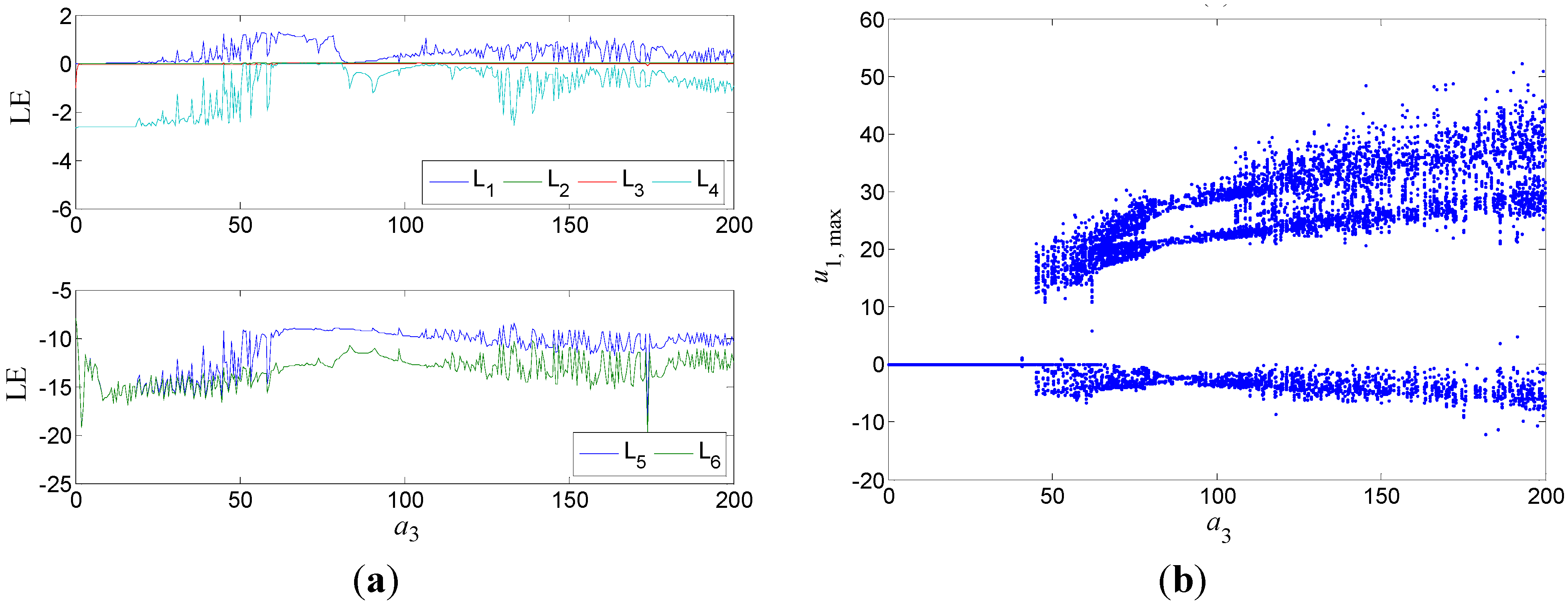
3.1. Dynamical Behaviors with Different Parameters

- (1)
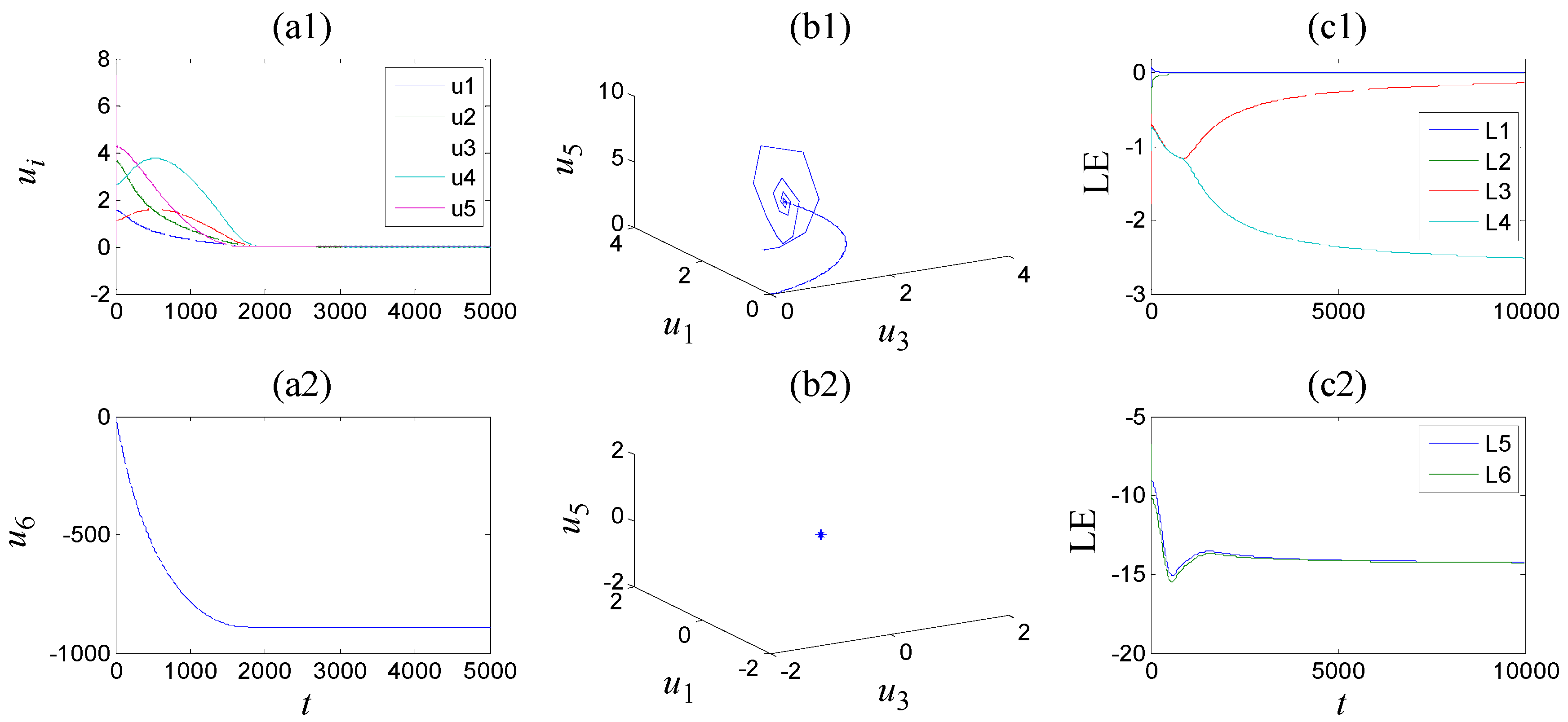
- Fixed points exist for . When , the system converges to a fixed point , and the six Lyapunov exponents are non-positive as shown in Figure 3.
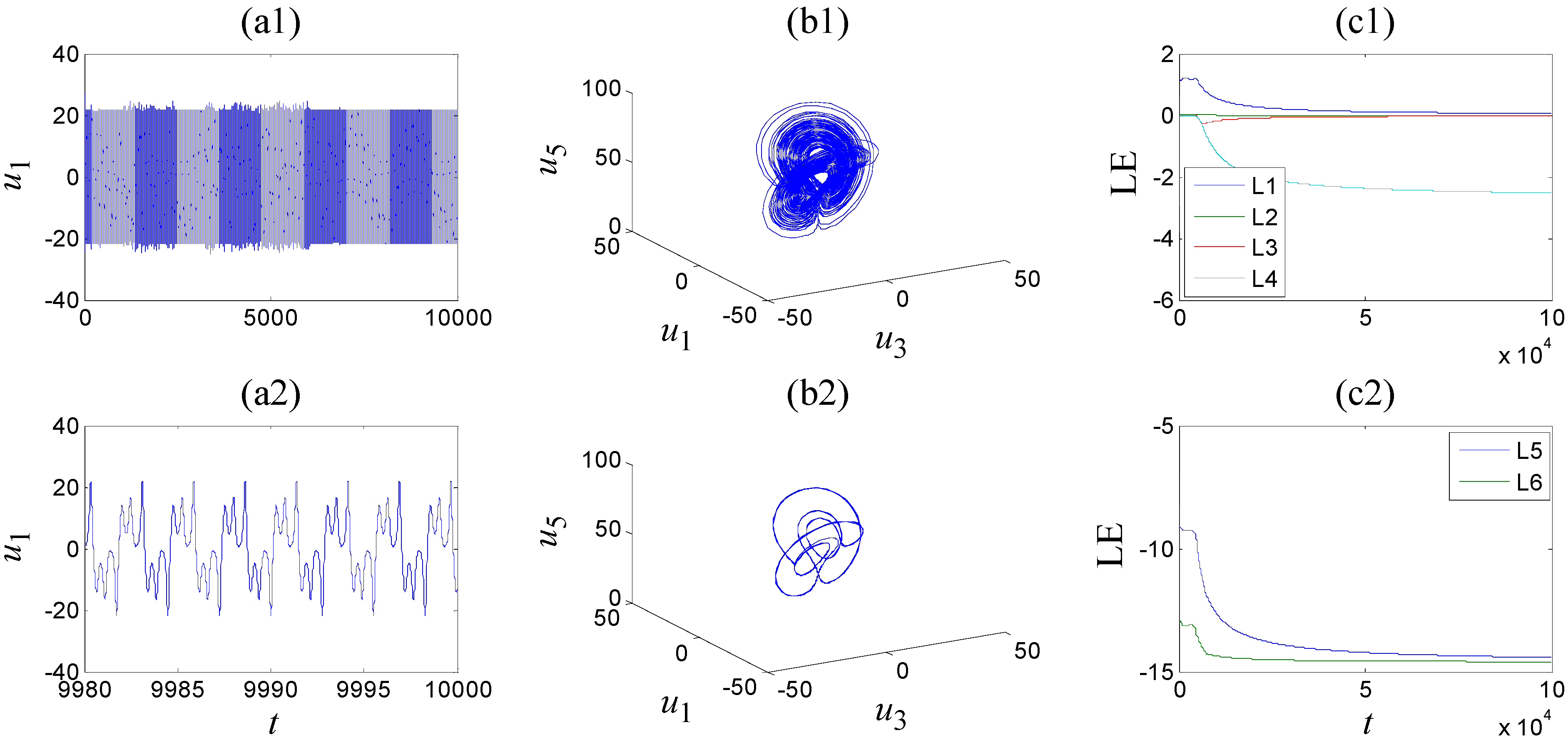
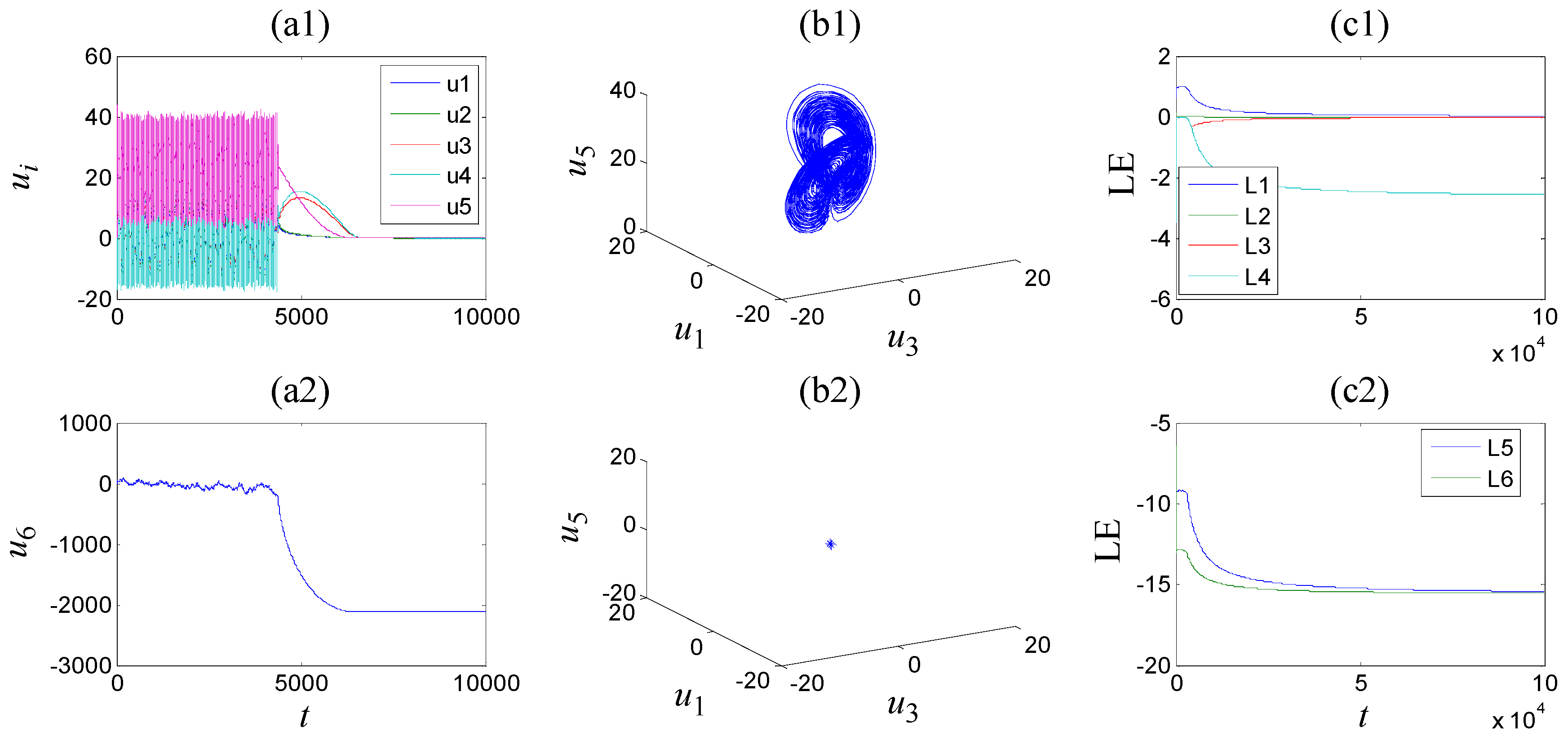
- (2)
- Transient chaos to fixed points exist for . When , the system goes through transient chaos and converges to fixed point as shown in Figure 4. One Lyapunov exponent (i.e., L1) is positive incipiently, and then tends to zero asymptotically.
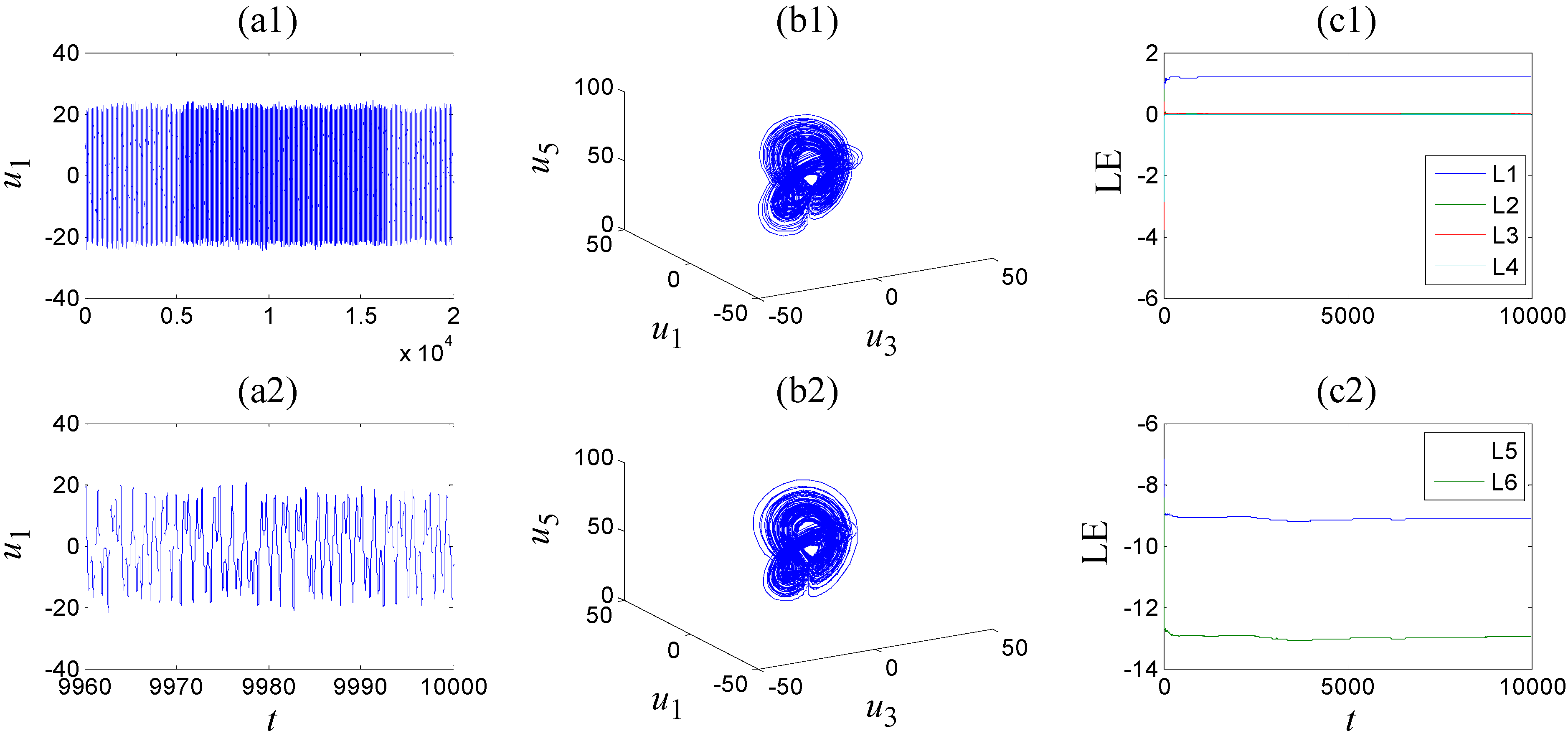
- (3)
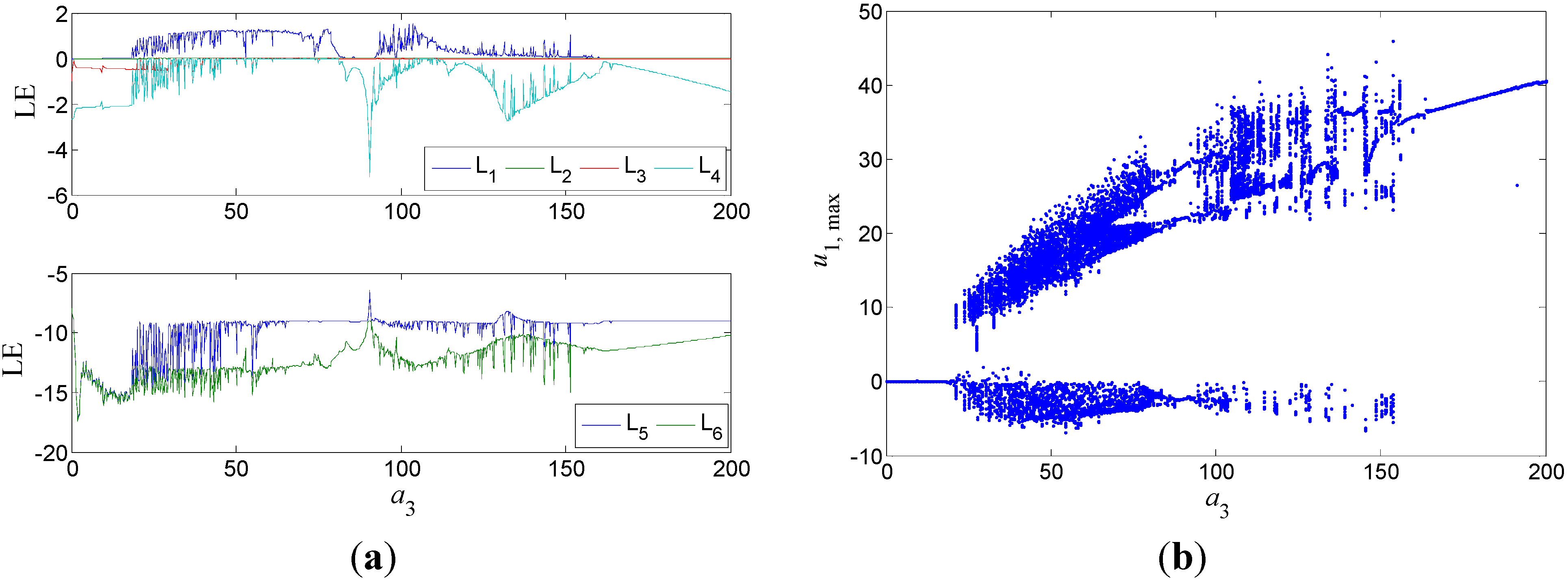
- A chaotic zone covers most region of . When , the system operates chaotically with a positive Lyapunov exponent as shown in Figure 5.
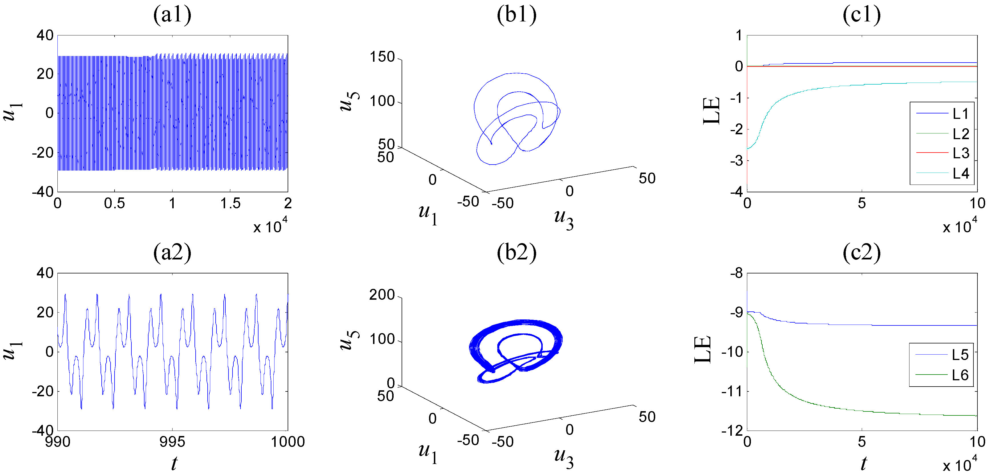
- (4)
- Transient chaos to Period-5 orbits exist in a narrow interval . When , the system goes through transient chaos and Period-5 orbit intermittently, and enters into the steady state of Period-5 eventually, as shown in Figure 6.
- (5)
- Transient Period-3 to tours exist for . When , the system operates in Period-3 orbit at first, and then enters into the state of tours as shown in Figure 7.
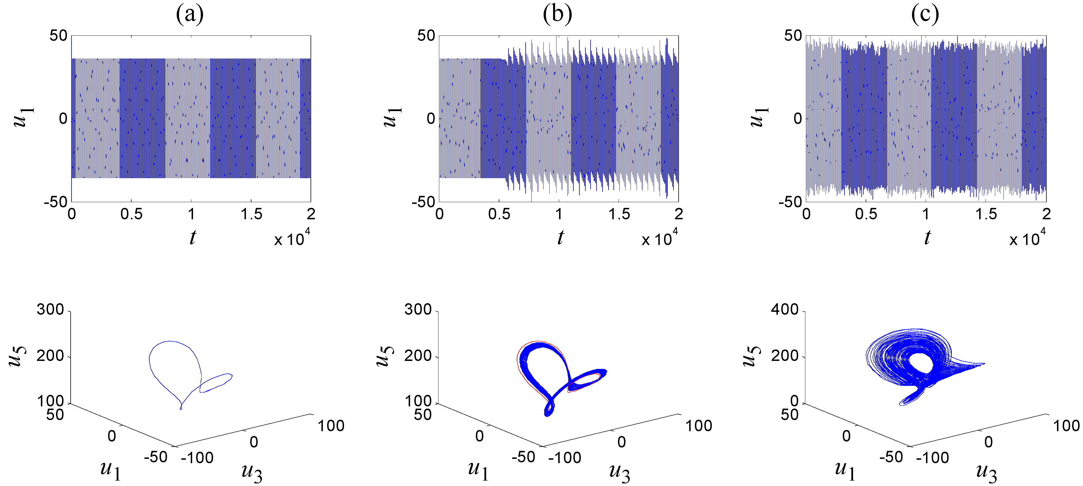
- (6)
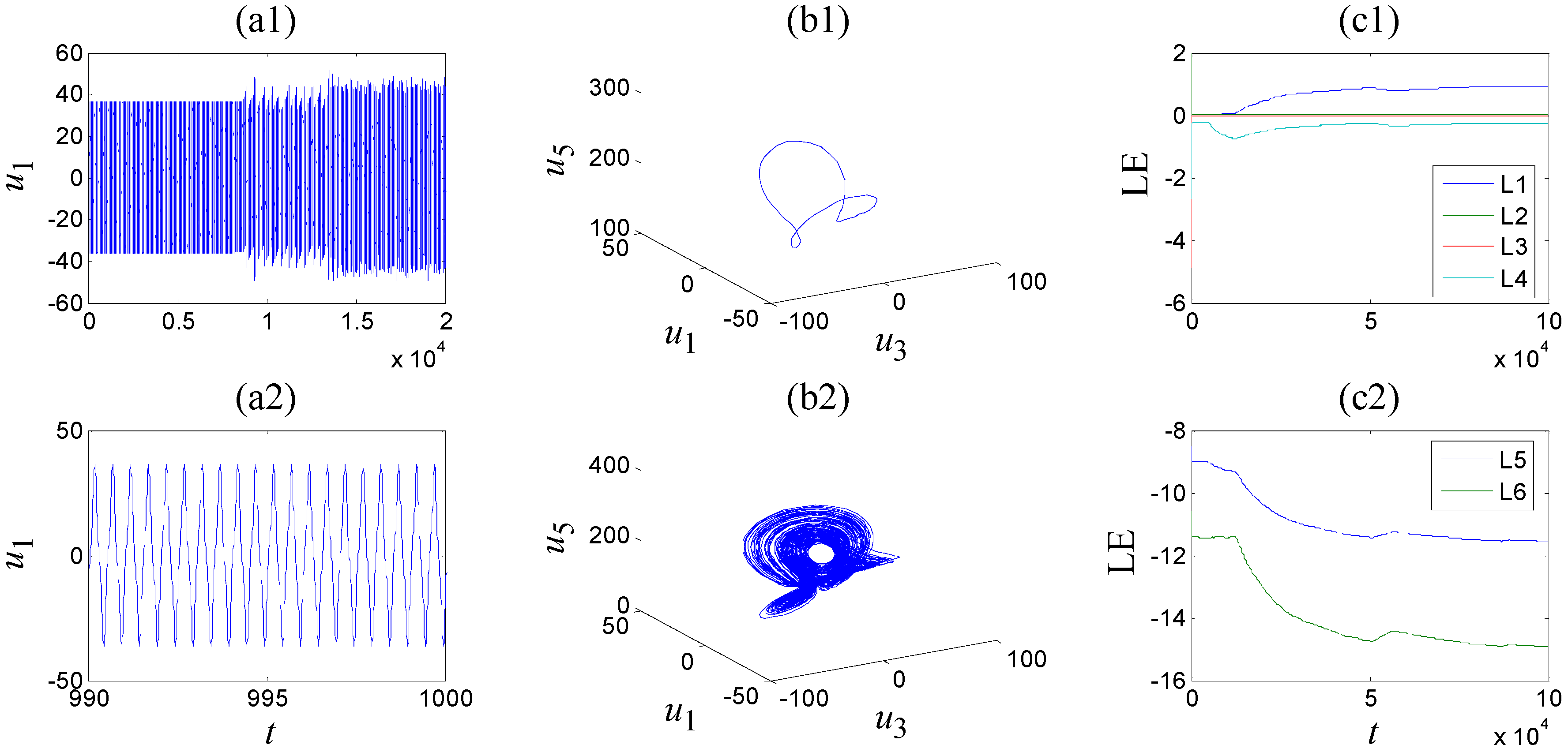
- Transient Period-1 to chaos exist for . When , as shown in Figure 8, in the beginning the system operates in Period-1 orbit, then enters into the state of tours, and slides into a chaotic state in the end. The Lyapunov exponent L1 changes from zero to a positive number.


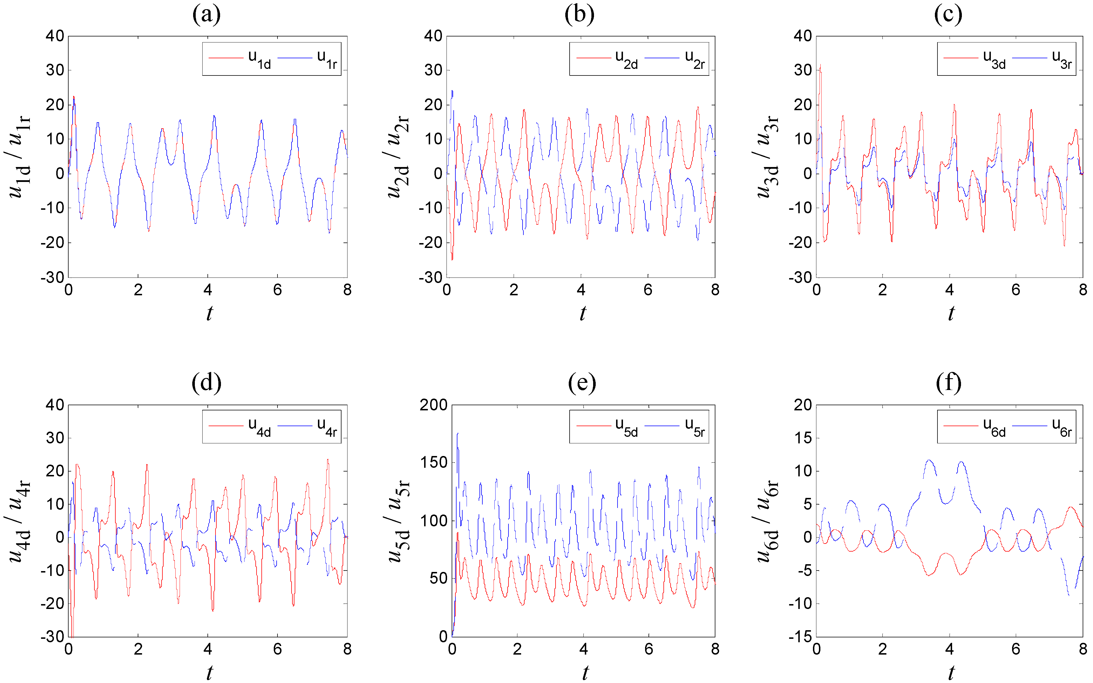
3.2. Dynamical Behaviors with Different Initial Conditions
4. MPS of the Memristor-Based Complex Lorenz System
4.1. MPS Design
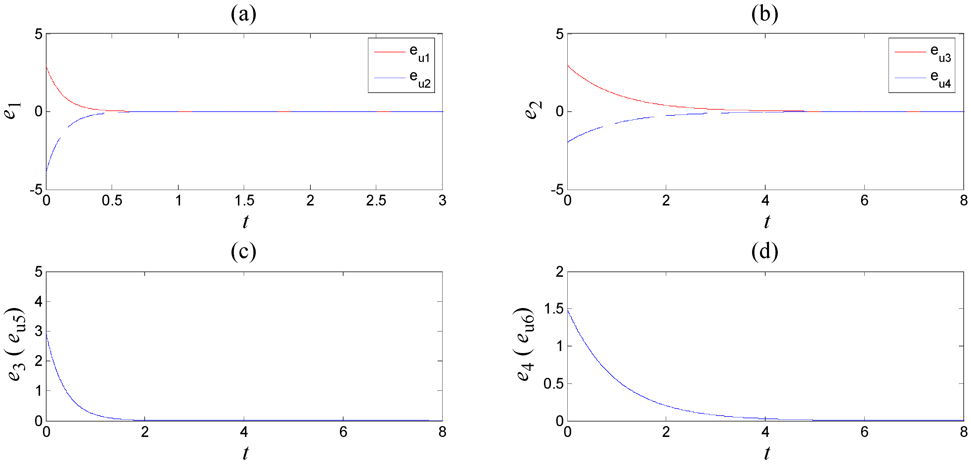
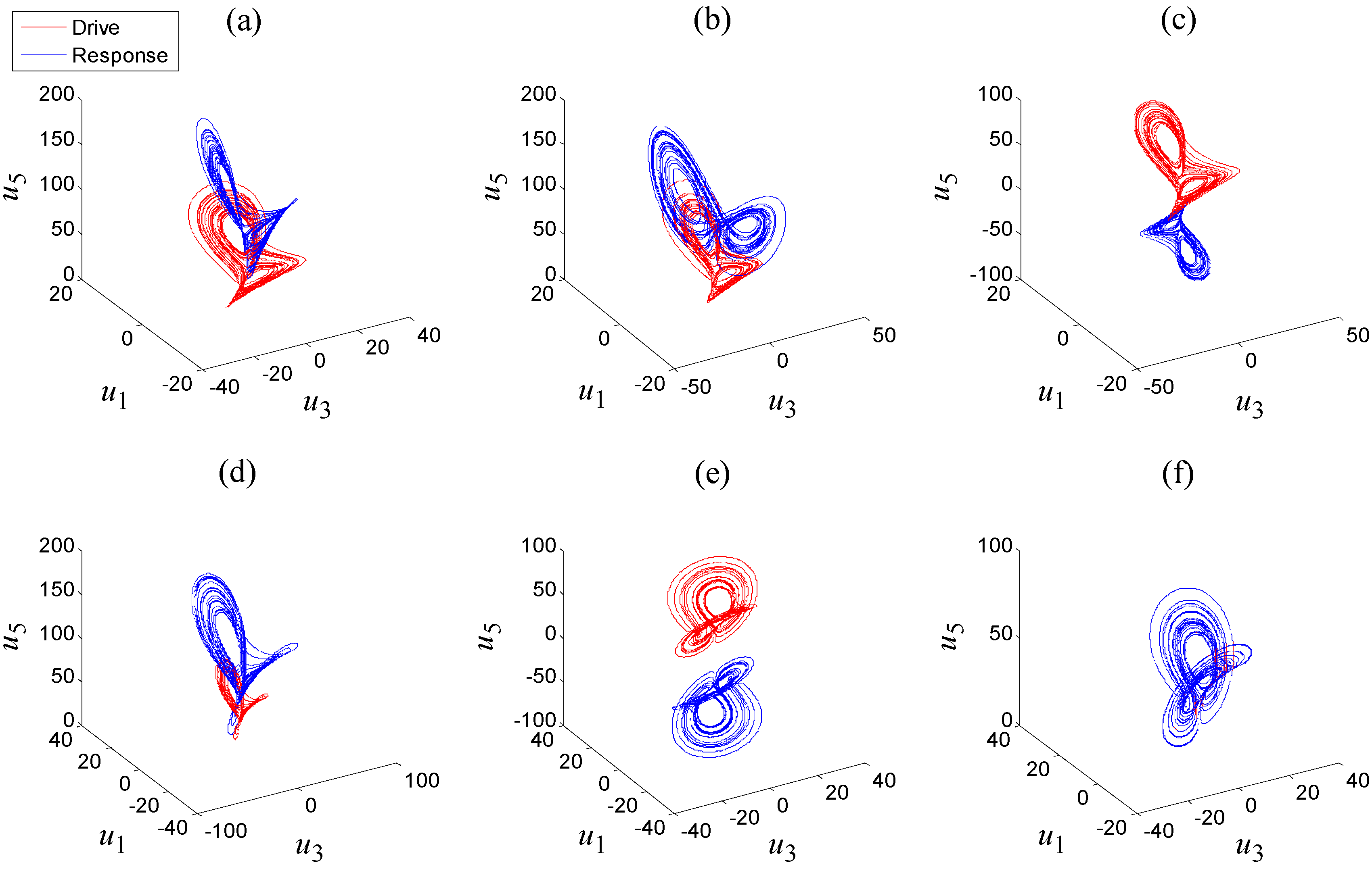
4.2. Numerical Simulations

5. Conclusions
Acknowledgments
Author Contributions
Conflicts of Interest
References
- Itoh, M.; Chua, L.O. Memristor Oscillators. Int. J. Bifurc. Chaos 2008, 18, 3183–3206. [Google Scholar] [CrossRef]
- Muthuswamy, B.; Kokate, P.P. Memristor-based chaotic circuits. IETE Tech. Rev. 2009, 26. [Google Scholar] [CrossRef]
- Messias, M.; Nespoli, C.; Botta, V.A. Hopf bifurcation from lines of equilibria without parameters in memristor oscillators. Int. J. Bifurc. Chaos 2010, 20, 437–450. [Google Scholar] [CrossRef]
- Li, Y.; Huang, X.; Guo, M. The generation, analysis, and circuit implementation of a new memristor based chaotic system. Math. Probl. Eng. 2013, 2013. [Google Scholar] [CrossRef]
- Ishaq Ahamed, A.; Lakshmanan, M. Nonsmooth bifurcations, transient hyperchaos and hyperchaotic beats in a memristive Murali–Lakshmanan–Chua circuit. Int. J. Bifurc. Chaos 2013, 23. [Google Scholar] [CrossRef]
- Wang, X.; Wang, G.; Wang, X. Dynamic character analysis of a LDR, memristor-based chaotic system. J. Circuits Syst. Comput. 2014, 23. [Google Scholar] [CrossRef]
- Lu, Y.; Huang, X.; He, S.; Wang, D.; Zhang, B. Memristor Based van der Pol oscillation circuit. Int. J. Bifurc. Chaos 2014, 24. [Google Scholar] [CrossRef]
- Wen, S.; Zeng, Z.; Huang, T.; Chen, Y. Fuzzy modeling and synchronization of different memristor-based chaotic circuits. Phys. Lett. A 2013, 377, 2016–2021. [Google Scholar] [CrossRef]
- Xi, H.; Li, Y.; Huang, X. Generation and nonlinear dynamical analyses of fractional-order memristor-based Lorenz systems. Entropy 2014, 16, 6240–6253. [Google Scholar] [CrossRef]
- Zhang, B.; Deng, F. Double-compound synchronization of six memristor-based Lorenz systems. Nonlinear Dyn. 2014, 77, 1519–1530. [Google Scholar] [CrossRef]
- Hu, X.; Chen, G.; Duan, S.; Feng, G. A memristor-based chaotic system with boundary conditions. In Memristor Networks; Adamatzky, A., Chua, L., Eds.; Springer: Berlin/Heidelberg, Germany, 2014; pp. 351–364. [Google Scholar]
- Li, Q.; Zeng, H.; Li, J. Hyperchaos in a 4D memristive circuit with infinitely many stable equilibria. Nonlinear Dyn. 2015, 79, 2295–2308. [Google Scholar] [CrossRef]
- Fitch, A.L.; Yu, D.; Iu, H.H.C.; Sreeram, V. Hyperchaos in a memristor-based modified canonical Chua’s circuit. Int. J. Bifurc. Chaos 2012, 22. [Google Scholar] [CrossRef]
- Ma, J.; Chen, Z.; Wang, Z.; Zhang, Q. A four-wing hyper-chaotic attractor generated from a 4-D memristive system with a line equilibrium. Nonlinear Dyn. 2015, 81, 1275–1288. [Google Scholar] [CrossRef]
- Chen, M.; Li, M.; Yu, Q.; Bao, B.; Xu, Q.; Wang, J. Dynamics of self-excited attractors and hidden attractors in generalized memristor-based Chua’s circuit. Nonlinear Dyn. 2015, 81, 215–226. [Google Scholar] [CrossRef]
- Bao, B.; Jiang, P.; Wu, H.; Hu, F. Complex transient dynamics in periodically forced memristive Chua’s circuit. Nonlinear Dyn. 2015, 79, 2333–2343. [Google Scholar] [CrossRef]
- Bao, B.-C.; Xu, J.-P.; Liu, Z. Initial state dependent dynamical behaviors in a memristor based chaotic circuit. Chin. Phys. Lett. 2010, 27. [Google Scholar] [CrossRef]
- Cafagna, D.; Grassi, G. On the simplest fractional-order memristor-based chaotic system. Nonlinear Dyn. 2012, 70, 1185–1197. [Google Scholar] [CrossRef]
- Teng, L.; Iu, H.H.C.; Wang, X.; Wang, X. Chaotic behavior in fractional-order memristor-based simplest chaotic circuit using fourth degree polynomial. Nonlinear Dyn. 2014, 77, 231–241. [Google Scholar] [CrossRef]
- Fowler, A.C.; Gibbon, J.D.; McGuinness, M.J. The complex Lorenz equations. Physica D Nonlinear Phenom. 1982, 4, 139–163. [Google Scholar] [CrossRef]
- Liu, J.; Liu, S.; Zhang, F. A novel four-wing hyperchaotic complex system and its complex modified hybrid projective synchronization with different dimensions. Abstr. Appl. Anal. 2014, 2014. [Google Scholar] [CrossRef]
- Luo, C.; Wang, X. Chaos generated from the fractional-order complex Chen system and its application to digital secure communication. Int. J. Mod. Phys. C 2013, 24. [Google Scholar] [CrossRef]
- Muthukumar, P.; Balasubramaniam, P.; Ratnavelu, K. Fast projective synchronization of fractional order chaotic and reverse chaotic systems with its application to an affine cipher using date of birth (DOB). Nonlinear Dyn. 2015, 80, 1883–1897. [Google Scholar] [CrossRef]
- Zhang, F. Lag synchronization of complex Lorenz system with applications to communication. Entropy 2015, 17, 4974–4985. [Google Scholar] [CrossRef]
- Sun, J.; Shen, Y.; Yin, Q.; Xu, C. Compound synchronization of four memristor chaotic oscillator systems and secure communication. Chaos Interdiscip. J. Nonlinear Sci. 2013, 23, 13140. [Google Scholar] [CrossRef] [PubMed]
- Balasubramaniam, P.; Muthukumar, P.; Ratnavelu, K. Theoretical and practical applications of fuzzy fractional integral sliding mode control for fractional-order dynamical system. Nonlinear Dyn. 2015, 80, 249–267. [Google Scholar] [CrossRef]
- Muthukumar, P.; Balasubramaniam, P.; Ratnavelu, K. Synchronization and an application of a novel fractional order King Cobra chaotic system. Chaos Interdiscip. J. Nonlinear Sci. 2014, 24, 033105. [Google Scholar] [CrossRef] [PubMed]
- Muthukumar, P.; Balasubramaniam, P.; Ratnavelu, K. Synchronization of a novel fractional order stretch-twist-fold (STF) flow chaotic system and its application to a new authenticated encryption scheme (AES). Nonlinear Dyn. 2014, 77, 1547–1559. [Google Scholar] [CrossRef]
- Muthukumar, P.; Balasubramaniam, P. Feedback synchronization of the fractional order reverse butterfly-shaped chaotic system and its application to digital cryptography. Nonlinear Dyn. 2013, 74, 1169–1181. [Google Scholar] [CrossRef]
- Wang, B.; Jian, J.; Yu, H. Adaptive synchronization of fractional-order memristor-based Chua’s system. Syst. Sci. Control Eng. 2014, 2, 291–296. [Google Scholar] [CrossRef]
- Wen, S.; Zeng, Z.; Huang, T. Adaptive synchronization of memristor-based Chua’s circuits. Phys. Lett. A 2012, 376, 2775–2780. [Google Scholar] [CrossRef]
- Zhou, X.; Xiong, L.; Cai, W.; Cai, X. Adaptive synchronization and antisynchronization of a hyperchaotic complex Chen system with unknown parameters based on passive control. J. Appl. Math. 2013, 2013. [Google Scholar] [CrossRef]
- Rakkiyappan, R.; Sivasamy, R.; Li, X. Synchronization of identical and nonidentical memristor-based chaotic systems via active backstepping control technique. Circuits Syst. Signal Process. 2015, 34, 763–778. [Google Scholar] [CrossRef]
- Yang, S.; Li, C.; Huang, T. Impulsive control and synchronization of memristor-Based chaotic circuits. Int. J. Bifurc. Chaos 2014, 24, 1450162. [Google Scholar] [CrossRef]
- Aly, S.; Al-Qahtani, A.; Khenous, H.B.; Mahmoud, G.M. Impulsive control and synchronization of complex Lorenz systems. Abstr. Appl. Anal. 2014, 2014. [Google Scholar] [CrossRef]
- El-Sayed, A.M.A.; Elsaid, A.; Nour, H.M.; Elsonbaty, A. Dynamical behavior, chaos control and synchronization of a memristor-based ADVP circuit. Commun. Nonlinear Sci. Numer. Simul. 2013, 18, 148–170. [Google Scholar] [CrossRef]
- Mahmoud, G.M.; Bountis, T.; AbdEl-Latif, G.M.; Mahmoud, E.E. Chaos synchronization of two different chaotic complex Chen and Lü systems. Nonlinear Dyn. 2009, 55, 43–53. [Google Scholar] [CrossRef]
- Zhou, P.; Bai, R.; Zheng, J. Projective synchronization for a class of fractional-order chaotic systems with fractional-order in the (1, 2) interval. Entropy 2015, 17, 1123–1134. [Google Scholar] [CrossRef]
- Huang, J.; Li, C.; Huang, T.; Wang, H.; Wang, X. Synchronization and lag synchronization of hyperchaotic memristor-based Chua’s circuits. Math. Probl. Eng. 2014, 2014. [Google Scholar] [CrossRef] [PubMed]
- Jin-E, Z. Combination-combination hyperchaos synchronization of complex memristor oscillator system. Math. Probl. Eng. 2014, 2014. [Google Scholar] [CrossRef]
- Zhou, X.; Jiang, M.; Huang, Y. Combination synchronization of three identical or different nonlinear complex hyperchaotic systems. Entropy 2013, 15, 3746–3761. [Google Scholar] [CrossRef]
- Chua, L.O. Memristor-The missing circuit element. IEEE Trans. Circuit Theory 1971, 18, 507–519. [Google Scholar] [CrossRef]
© 2015 by the authors; licensee MDPI, Basel, Switzerland. This article is an open access article distributed under the terms and conditions of the Creative Commons Attribution license (http://creativecommons.org/licenses/by/4.0/).
Share and Cite
Wang, S.; Wang, X.; Zhou, Y. A Memristor-Based Complex Lorenz System and Its Modified Projective Synchronization. Entropy 2015, 17, 7628-7644. https://doi.org/10.3390/e17117628
Wang S, Wang X, Zhou Y. A Memristor-Based Complex Lorenz System and Its Modified Projective Synchronization. Entropy. 2015; 17(11):7628-7644. https://doi.org/10.3390/e17117628
Chicago/Turabian StyleWang, Shibing, Xingyuan Wang, and Yufei Zhou. 2015. "A Memristor-Based Complex Lorenz System and Its Modified Projective Synchronization" Entropy 17, no. 11: 7628-7644. https://doi.org/10.3390/e17117628