1. Introduction
Nowadays, the development of society is becoming more and more complicated and networked; thus, complex networks have emerged and aroused much attention [
1]. A complex network is a structure that is made up of a large set of nodes (also called vertices, oscillators, agents) that are inter-connected to varying extents by a set of links (also called edges). Complex networks, indeed, are so ubiquitously found in nature and in the modern world that it is absolutely essential for us to have a thorough understanding of their dynamical behavior (for example, coupled biological systems, such as neural networks, and socially-interacting animal species [
2]), and complex network synchronization holds particular promise for applications to many fields (for example, population dynamics [
2,
3], power systems [
4,
5] and automatic control [
6]).
Synchronization is a process in which two or more dynamical systems seek to adjust a certain prescribed property of their motion to a common behavior in the limit as time tends to infinity [
7]. It is a phenomenon that has been widely investigated since it was discovered by Pecora and Carroll in 1990 [
8]. Many synchronization patterns have been explored (for example, complete synchronization [
9,
10,
11], cluster synchronization [
12,
13], phase synchronization [
14], partial synchronization [
15], projective synchronization [
16,
17]), and synchronization can be achieved by the use of pinning control [
18,
19], adaptive control [
20,
21,
22], intermittent control [
23], impulsive control [
24,
25], fuzzy control [
26], hybrid control [
27] or active control [
28].
In the study of synchronization, inner synchronization is a synchronous phenomenon within a network and denotes the behavior of all of the nodes among one complex network becoming synchronous. Many different cases for inner synchronization have been investigated so far [
4,
5,
6,
7,
8,
9,
10,
11,
12,
13,
14,
15,
16,
17,
18,
19,
20,
21,
22,
23,
24,
25,
26,
27,
28] On the contrary, outer synchronization [
29,
30] is a synchronous phenomenon between networks, that is to say it refers to the synchronization occurring between two or more coupled complex networks regardless of the occurrence of inner synchronization, and many phenomena can be explained by outer synchronization in nature, such as an infectious disease spreading between different communities and different species’ development in balance [
30]. Li
et al. first proposed the concept of outer synchronization and derived analytically a criterion for the synchronization of two networks that have the same topological connectivity in 2007 [
30]. Additionally, outer synchronization between two coupled discrete-time networks that have the same connection topologies was derived analytically [
31]. On the other hand, the problem of generalized outer synchronization between two completely different complex dynamical networks was investigated in [
32]. The outer synchronization between two delay-coupled complex dynamical networks with nonidentical topological structures and a noise perturbation was regarded in [
33]. However, there still exists the situation that the complex networks cannot achieve synchronization.
Stochastic perturbations and time delays are important considerations when simulating realistic complex networks, because signals traveling along real physical systems are usually randomly perturbed by the environmental elements [
21]. In fact, signals transmitted between nodes of complex networks are unavoidably subject to stochastic perturbations from the environment, which may cause information contained in these signals to be lost [
34]; the distance and finite speed of information transmission between pairs of nodes may cause time delays. Some results have recently appeared on the synchronization of complex networks with coupling delays [
35,
36,
37] and stochastic perturbations [
38,
39,
40,
41].
Because of the complexity of complex networks, pinning control is a technique that applies controllers to only a small fraction of the nodes in a network, and the technique is important because it greatly reduces the number of controlled nodes for real-world complex networks (which, in most cases, is huge). In fact, pinning control can be so effective for some networks that a single pinning controller is required for synchronization; namely, for complex networks that have either a symmetric or an asymmetric coupling matrix [
18]. Other pinning schemes, on the other hand, are capable of globally- and exponentially-stabilizing a network into a homogeneous state by using an optimal combination of the number of pinned nodes and the feedback control gain [
19].
Motivated by the above discussions, in this paper, we study the mean square exponential synchronization of two nonidentical stochastic time-varying delayed complex networks by using the pinning control method. Some sufficient conditions are derived for mean square exponential synchronization of these networks by applying the Lyapunov–Krasovskii functional method. Our results will be applicable to many synchronization problems in different fields of science and technology.
The paper is organized as follows. In
Section 2, a general model of two different stochastic complex networks with both time-varying delay dynamical nodes and time-varying delay coupling and some preliminaries are given. In
Section 3, some exponential synchronization criteria for such complex dynamical networks are established. In
Section 4, a numerical example for verifying the effectiveness of the theoretical results is provided. We conclude the paper in
Section 5.
2. Preliminaries
2.1. Notations
Throughout this paper, shall denote the n-dimensional Euclidean space and the set of all real matrices. The superscript T shall denote the transpose of a matrix or a vector; denotes the trace of the corresponding matrix, and ; and denotes the n-dimensional identity matrix. For square matrices M, the notation (respectively, ) shall mean that M is a positive-definite (respectively, negative-definite) matrix, and and shall denote the greatest and least eigenvalues of a symmetric matrix, respectively. Let be a complete probability space with a filtration that is right continuous with containing all of the -null sets. shall denote the family of continuous functions ϕ from to with the uniform norm and the family of all measurable, -valued stochastic variables , such that , where stands for the correspondent expectation operator with respect to the given probability measure .
2.2. Network Model
Consider a complex network consisting of
N identical linearly- and diffusively-coupled nodes with non-delayed and time-varying-delayed linear coupling. Additionally, every node in the network is an
n-dimensional dynamical unit. Then, the network model of the drive system can be denoted as:
where
is the state vector of the
i-th node of the network,
is a continuous vector-valued function and
is an inner coupling of the networks that satisfies
,
. Here,
and
are the outer coupling matrices of the network at time
t and
, respectively, such that
for
,
,
for
and
.
is the inner time-varying delay satisfying
, and
is the coupling time-varying delay satisfying
. Finally,
, and
is a bounded vector-form Wiener process, satisfying:
Compared to the drive system mentioned, the response complex network is denoted as consisting of
M identical linearly- and diffusively-coupled nodes with non-delayed and time-varying-delayed linear coupling. Additionally, every node in the network is an
n-dimensional dynamical unit:
where
is the state vector of the
j-th node of the response network and
is a continuous vector-valued function. Here,
and
are the outer coupling matrices of the network at time
t and
, respectively, such that
for
,
,
for
and
. In this paper,
and
are assumed to be irreducible in the sense that there are no isolated nodes.
The initial conditions associated with Equation (
2) are:
where
,
with the norm
.
2.3. Some Definitions, Lemmas and Assumptions
In the following, we present some definitions and lemmas that will be required throughout this paper.
Definition 1. The drive network (
2) and the response network (
1) are said to be exponentially synchronized in the mean square if the trivial solutions of Systems (
2) and (
1) are such that:
for some
and some
for any initial data
.
Definition 2. [
21] A continuous function
is said to belong to the function class QUAD, denoted by
for some given matrix
, if there exists a positive definite diagonal matrix
, a diagonal matrix
and constants
,
, such that
satisfies the condition:
for all
.
Almost all of the well-known chaotic systems belong to the function class QUAD, such as the Lorenz system, the Rössler system, the Chen system, the delayed Chua’s circuit, the delayed Hopfield neural network and the logistic delayed differential system [
21,
23].
Lemma 1. Consider an
n-dimensional stochastic differential equation:
Let
denote the family of all nonnegative functions
on
, which are twice continuously differentiable in
x and once differentiable in
t. If
, define an operator
form
to
by:
where
,
,
. If
, then for any
,
as long as the expectations of the integrals exist [
42,
43].
The following assumptions will be used throughout this paper for establishing the synchronization conditions.
- H1
and are bounded and continuously differentiable functions, such that , , and . Let
- H2
Let
. Then, there exist positive definite constant matrices
,
and
for
and
, such that:
where
.
Remark 1. The assumptions are common in the literature on stochastic complex networks with time-varying delay, such as [
21,
23,
27,
38,
39,
40]. Assumption H1 restricts the time delay, and Assumption H2 restricts the noise strength. We shall simply write:
3. Main Result
In the paper, the synchronization between the drive network (
1) and the response network (
2) will be investigated. In order to reach the synchronization, some extra controllers are required to add on the partial nodes of the response system. Without loss of generality, let the first
l nodes in the response system be controlled. Additionally, the response network with a control scheme is given by:
where
(
) are the linear state feedback controllers that are defined by:
where
(
) are the control gains, denoted by
. Define
(
,
) as the synchronization error. Then, according to the controller (
7), the error system is:
Remark 2. The pinning controllers (
7) are added to a part of the node in response networks by the information of the first node in drive networks, which is easy to achieve. The drive networks (
1) and response networks (
2) reach outer synchronization in the mean square by pinning controllers (
7) as long as error System (
8) is globally and exponentially stable in the mean square.
We present the outer synchronization criteria for two stochastic complex networks with time-varying delay.
Theorem 1. Let Assumptions H1 and H2 be true, and let
. If there exist
α,
β,
and
, such that:
where:
then the solutions
(
,
) of System (
8) are globally and exponentially stable in the mean square.
Proof. Define the Lyapunov–Krasovskii function:
By Lemma 1, we have:
For simplicity, denote ; ; .
Because
, we get:
From the definitions of
(
), the following equation holds:
Similarly,
By using
for any
and
, we can obtain:
and:
where and .
Denote
; we have:
Using Assumption H2, we get:
Substituting Inequalities (
12)– (
18) into Equality (
11), we have:
By Equation (
10), we get:
Define:
where constant
will be decided later, and use Equation (
21) to compute the operator:
which, after applying the generalized Itô’s formula, gives:
for any
. Hence, we have:
which, by using the change of variables
, gives:
and a further change of variables
gives:
Substituting Inequalities (
23) and (
24) into Equality (
22), we have:
By Condition (
9), this equation:
has at least one positive root. Let
γ be the smallest positive root of (
25). Therefore, we obtain:
so that:
where
. The proof is hence complete. ☐
Remark 3. Inequality (
9) relies on the coupled matrices, the dynamics system, the noise strength and the time delays. The linear matrix inequality method is inadequate for assessing the stability of the synchronous solution.
When the time-varying delays are constant (
i.e.,
,
), we obtain the following corollary:
Corollary 1. Let Assumptions H1 and H2 be true, and let
. If there exist
and
, such that:
where:
then the solutions
(
,
) of System (
8) are globally and exponentially stable in the mean square.
When
, we can get the following corollary:
Corollary 2. Let Assumptions H1 and H2 be true, and let
. If there exist
and
, such that:
where:
then the solutions
(
,
) of System Equation (
8) are globally and exponentially stable in the mean square.
When
,
and
, we can get the following corollary:
Corollary 3. Let Assumptions H1 and H2 be true, and let
. If there exist
and
, such that:
where:
then the solutions
(
,
) of System (
8) are globally and exponentially stable in the mean square.
4. Numerical Simulation
In this section, we present some numerical simulation results that validate the theorem of the previous section.
Consider the 2D chaotic delayed neural network:
where
,
,
and
Taking
and
, we have
and
, so that Condition (
3) is satisfied [
21]. Thus:
and:
where:
,
,
and
Computations then yield
,
,
,
,
for
, and
. Then, the solutions of Equalities (
10) are:
,
,
; after solving Equation (
25), we obtain
, so that the conditions of Theorem 1 are satisfied.
The initial conditions for this simulation are
,
,
,
,
and for all
. The numerical approximation to the solution of stochastic differential Equation (
27) and Equation (
28) are found by the Euler–Maruyama method [
44] with
, and the trajectories of the pinning control gains are shown in
Figure 1,
Figure 2 and
Figure 3.
Figure 4 shows the time evolution of the synchronization errors without pinning control. One can see that the pinning control directly affects the synchronization of two complex network, which cannot be reached without pinning control.
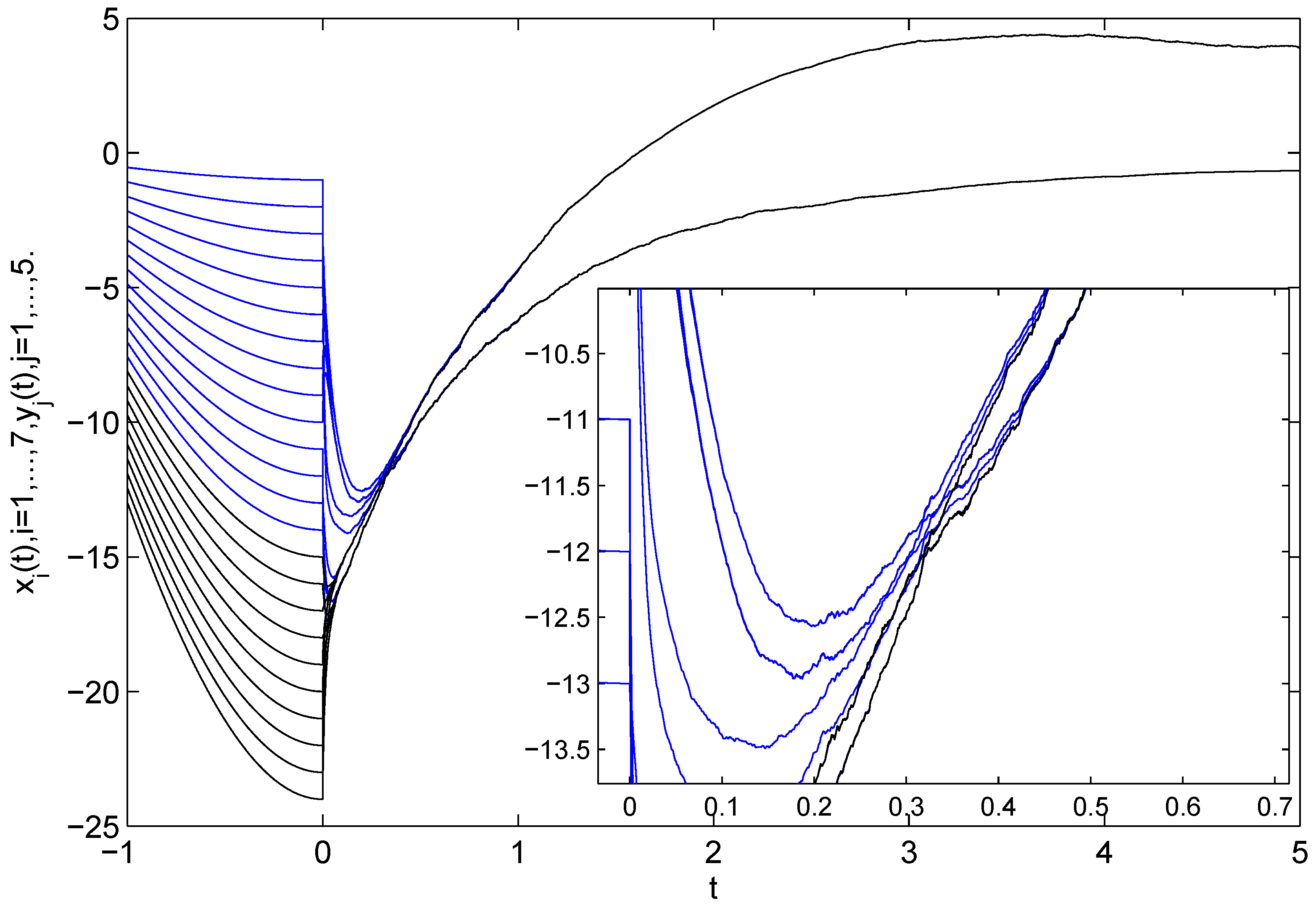
Figure 1.
The trajectories of the state variables of
and
(
and
) in Systems (
27) and (
28) under pinning control. The blue lines show the evolution of the driver systems, and the black lines represent the trajectory of the driver systems in the figure, as they do for the following figures.
Figure 1.
The trajectories of the state variables of
and
(
and
) in Systems (
27) and (
28) under pinning control. The blue lines show the evolution of the driver systems, and the black lines represent the trajectory of the driver systems in the figure, as they do for the following figures.
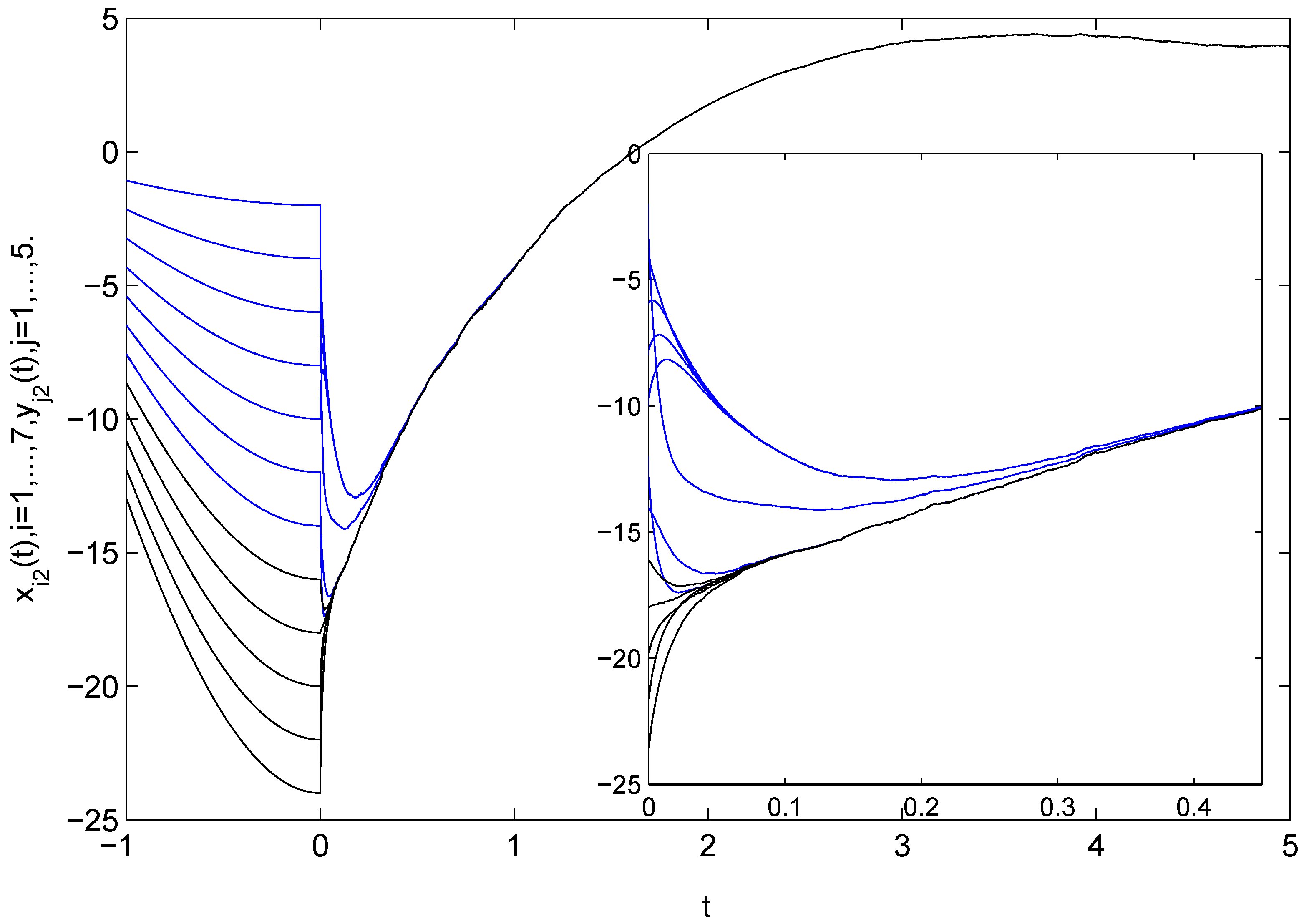
Figure 2.
The time evolution of
and
(
and
) in Systems (
27) and (
28) under pinning control.
Figure 2.
The time evolution of
and
(
and
) in Systems (
27) and (
28) under pinning control.
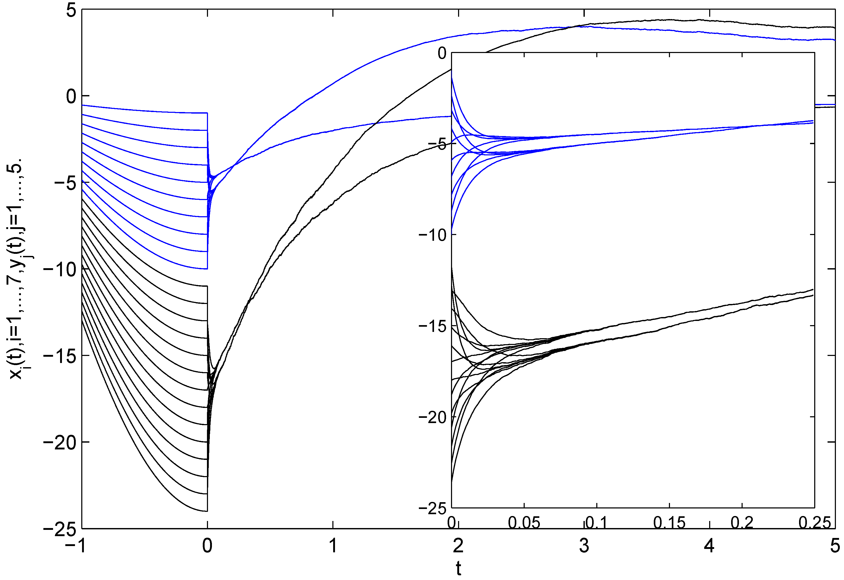
Figure 3.
The time evolution of
and
(
and
) in Systems (
27) and (
28) under pinning control.
Figure 3.
The time evolution of
and
(
and
) in Systems (
27) and (
28) under pinning control.
Figure 4.
The time evolution of
and
(
) in Systems (
27) and (
28) without pinning control.
Figure 4.
The time evolution of
and
(
) in Systems (
27) and (
28) without pinning control.


