Two-Dimensional Lattice Boltzmann for Reactive Rayleigh–Bénard and Bénard–Poiseuille Regimes

Abstract

We perform a computer simulation of the reaction-diffusion and convection that takes place in Rayleigh–Bénard and Bénard–Poiseuille regimes. The lattice Boltzmann equation (LBE) is used along with the Boussinesq approximation to solve the non-linear coupled differential equations that govern the systems’ thermo-hydrodynamics. Another LBE, is introduced to calculate the evolution concentration of the chemical species involved in the chemical reactions. The simulations are conducted at low Reynolds numbers and in terms of steady state between the first and second thermo-hydrodynamics instability. The results presented here (with no chemical reactions) are in good agreement with those reported in the scientific literature which gives us high expectations about the reliability of the chemical kinetics simulation. Some examples are provided.

1. Introduction

The Rayleigh–Bénard convection phenomenon is common in nature, governing various phenomena such as atmospheric fronts [1], thermal inversion (Bénard–Marangoni), ocean currents [2], circulation of the mantle [3], etc. In the chemical industry, convective rolls are present in the chemical and electrochemical reactors [4], fuel cells, distillation columns, selective membranes, ion exchange, among others. To characterize these phenomena in complex systems, a wide variety of numerical methods have been used: such as the finite element [5,6,7,8] and finite differences [9,10], among others.

Other methods of statistical physics have also been successfully used, such as Monte Carlo algorithms in the study of microscopic aspects of the Rayleigh–Bérnard dynamics as a phase transition [11,12]. Recently, the Lattice Boltzmann Method (LBM) has emerged [13,14] as one of the most powerful tools to describe complex thermos-hydrodynamic system [15,16,17]. The introduction of the BGK collision operator approach permits to significantly simplify the LB algorithm, although at some expenses of numerical stability in very low viscous regimes. Most importantly, in LBM the transport (free-streaming) is linear and can be dealt with exactly, while diffusion emerges from the relaxation dynamics of the collision operator, which is fully local. These are major advantages over macroscopic formulations of hydrodynamics.

When a fluid is heated from below and the Reynolds number is small, the heat transfer takes place by conduction. However, if a critical value is exceeded, natural convection is the predominant phenomena. The so-called Rayleigh–Bénard convection occurs due to the competition between the gravity and buoyant forces, creating instabilities in the fluid, which induces convective currents.

There are two thermo-convective instabilities in the Rayleigh–Bénard systems [18]. The first corresponds to the transition from a steady-state thermal conduction towards a state of thermal convection, formed by well-defined bidimensional stationary rollers. This transition occurs, theoretically, at a Rayleigh number of 1707.76, regardless of the value of the Prandtl number. The second transition occurs when the Rayleigh value increases until it can be considered a function of the Prandtl number. It consists of a bifurcation from a single frequency oscillating state, to a quasiperiodic double frequency flow. An additional increment of the Rayleigh number leads to a chaotic regime in a fully developed turbulence. Recently, a large number of articles with regard to the LBM applied on Rayleigh–Bénard convection, mainly between the first and second transition, where the Boussinesq approximation is valid, have been published. The first approach to Rayleigh–Bérnard systems by LBM is introduced by 1993 [19,20].

Many theoretical and experimental results restricted to low Reynolds and Rayleigh numbers have shown that layered Bénard–Poiseuille flow remains also stable, as long as the Prandtl number does not exceed a critical value. There are several articles based on finite differences [3,4,10] and in LBM [21] that have to do with the theory and numeric of this type of flow analysis. However, so far, there are few publications related to reactive systems under Rayleigh–Bénard and Bénard–Poiseuille regimes despite their importance among the applications above mentioned [22].

In order to simulate the dynamics of chemical reactions in two-dimensional systems with thermal and convective phenomena, a D2Q9 LBM is used in this paper at mesoscopic scale by taking into account (virtual) particles which move synchronously in a regular lattice, in accordance with discrete time steps. Then, when these particles reach simultaneously the same node of this lattice, they interact among themselves following collision rules that comply with the principles of mass, momentum and energy conservation, recovering in the macroscopic limit (through multiscale expansion), a number of differential equations, relying on the described phenomena. After the interaction, which is assumed to be instantaneous, the particles are scattered through first or second neighbors in the lattice. These define a distribution function of pseudo-particles f_i; namely, the probability that a particle is in a site-specific lattice node at time t, moving with speed c_i [23,24]. There are several other researches on coupled chemical reactions (electrokinetic) and reactive transport within micropores using mesoscopic modeling [25]. Pioneer work in the study of chemical kinetics using LBM has also been considered in this paper [26,27,28]. We perform a simulation in the Rayleigh–Bénard and Bénard–Poiseuille regimes for the Nitrous Oxide decomposition where Boussinesq approximation is valid, introducing the chemical kinetics as a function of the temperature via the Arrhenius law.

2. Thermal Decomposition of Nitrous Oxide

In this section, we address two different cases; the first pertains to the thermal decomposition of nitrous oxide (so called laughing gas) in the bulk of a fluid containing air plus the different species involved in this well characterized chemical reaction. This fluid performs a laminar flow through a rectangular open channel. The second case is similar but in a closed cavity; namely, the Rayleigh–Bénard and Bénard–Poiseuille regimes. See Figure 1.

Figure 1. The non-isothermal closed and open cavities used in this paper.

Figure 1. The non-isothermal closed and open cavities used in this paper.

In 1903, Boussinesq noted that when the differences of temperature were small, the thermodynamic properties of the fluid, such as the viscosity, the thermal diffusivity and the specific heat were also small, thus the fluid was approximately incompressible, while buoyant fluid effects were significant. This is due to the fact that the acceleration of the fluid is considerably less than the gravitational acceleration. Namely, the product of the gravity acceleration g and a small density difference is not negligible compared to other terms in the vertical movement component of the fluid in the Navier–Stokes equation. Boussinesq proposed an equation of state in which the fluid density is a linear function of the temperature and does not depend on the pressure. Following this hypothesis, the nonlinear coupled partial differential equations governing the thermos-hydrodynamic instability are as follows [29].

• The continuity equation

  $${\partial }_t\rho +\Delta \cdot \rho u=0$$

  (1)
• The Navier–Stokes equation with buoyant forces (G).

  $$\rho [{\partial }_{t}u+u\nabla \cdot u]=-\nabla \cdot \tau -\nabla \cdot P+G$$

  (2)
• The infinitesimal balance of heat transfer, based on the Fourier’s law, including effects of natural convection and viscous dissipation.

  $${\partial }_t\left(\rho C_{p}T\right)=\nabla \cdot k_T\nabla T-\nabla \cdot \rho uT-\tau :\nabla u$$

  (3)
• The linear Bousinesq equation of state.

  $$\rho ={\rho }_0[1-\beta \left(T-T_0\right)]$$

  (4)

In these equations ρ, C_p and k_T are the density, heat capacity and thermal conductivity of the fluid, respectively. Besides, u, P and T are the speed, pressure and temperature of the fluid; τ is the molecular momentum flux tensor. In this paper, we use the dimensionless version of Equations (1)–(3), namely;

$${\nabla }^{\ast }\cdot u^{\ast }=0$$

(5)

$$\frac{1}{\mathrm{Pr}}\left[\frac{\delta u^{\ast }}{\delta t^{\ast }}+u^{\ast }\cdot \nabla u^{\ast }+\nabla P^{\ast }\right]-{\nabla }^{{\ast }^2}{u}^{\ast }-\sqrt{Ra}{T}^{\ast }{y}^{\ast }=0$$

(6)

$$\frac{\delta T^{\ast }}{\delta t}+u^{\ast }\cdot {\nabla }^{\ast }{T}^{\ast }-\sqrt{Ra}{u}^{\ast }\cdot y^{\ast }-{\nabla }^{{\ast }^2}{T}^{\ast }=0.$$

(7)

where Ra, Pr are the Reynolds and Prandtl dimensionless numbers.

The chemical dynamics are governed by the following equation of reaction-diffusion and convection is used in this paper.

$${\partial }_t{C}_i=\nabla \cdot D_i\nabla C_i-u\cdot \nabla C_i+R_Q$$

(8)

The left side of this equation represents the changes of the chemical species in accordance to the concentration of i. Meanwhile, on the right side for each species i, the first term corresponds to the molar diffusion flux, with D_i as the diffusion coefficient; the second term represents the convective transport drew by currents of fluid moving with speed u; finally, the third term corresponds to the speed of the different species production by the chemical reaction. This equation is considered in dimensionless form.

Equations (5)–(8) are a set of nonlinear differential equations, regardless of the nature of the chemical reaction, that pose a serious challenge to its resolution.

The decomposition of the laughing gas is considered as an example in this paper:

$${\text{N}}_2\text{O}\to {\text{N}}_2+\frac{1}{2}{\text{O}}_2$$

(9)

Experimental evidence indicates that the corresponding chemical kinetics is given by [28]

$$R_Q=-r_{{\text{N}}_2\text{O}}=\frac{k_1{\left[{\text{N}}_2\text{O}\right]}^2}{1+k_2\left[{\text{N}}_2\text{O}\right]}.$$

(10)

here k₁ and k₂ are constants obtained through experiments. Obviously, the N₂O decomposition is not elemental; i.e. if we assume that two molecules of N₂O collide and spontaneously disappear, at certain required conditions, becoming two molecules of N₂ and one of O₂, then the kinetics should be $R_Q=-r_{{\text{N}}_2\text{O}}=k{\left[{\text{N}}_2\text{O}\right]}^2$, which experimentally is not the case. Thus, this is a non-elemental chemical reaction and needs a new proposed mechanism for itself; namely, a set of elemental reactions take place at the decomposition rate. At a fixed temperature, it is proportional to the collision of molecules (or the spontaneous decomposition of one molecule), and also proportional to the concentration of the species involved. In such a case, we must introduce some molecular non-stable structures (they are produced and immediately consumed in another elemental reaction) whose concentration cannot be measured by experiments and are small enough to have a rate of production (or decomposition) equal to zero. These structures are called intermediate complex chemical states.

We propose the following reaction mechanism that suits this kinetics as follows:

$$2{\text{N}}_2\text{O}\underset{k_{2\text{'}}}{\overset{k_{1\text{'}}}{{\displaystyle \rightleftarrows }}}{X}^{\ast }+{\text{N}}_2\text{O}$$

(11)

$$X^{\ast }\stackrel{k_{3\text{'}}}{\to }{\text{N}}_2+\frac{1}{2}{\text{O}}_2.$$

(12)

here, $k_{1\text{'}}$, $k_{2\text{'}}$, $k_{3\text{'}}$ are theoretical constants (k₁ and k₂ are related with these hypothetical constants). Equations (11) and (12) are added together to build the chemical reaction (9) experimentally obtained and are assumed to be elemental, so we have four differential equations (one for each rate of production or decomposition of the species; N₂O, X^*, N₂ and O₂) and the corresponding algebraic equations obtained by stoichiometry; thus it is possible to write, in this mechanism, the global N₂O decomposition rate only in terms of the N₂O concentration. From the full set of available equations all species’ concentrations and rates follow. In the first step of our mechanism (Equation (11)), N₂O disappears following Equation (13), and it may be noted that we deal with this as elemental kinetics.

$$-\frac{d\left[N_{2}O\right]}{dt}=k_{1\text{'}}{\left[{\text{N}}_2\text{O}\right]}^2-k_{2\text{'}}\left[{\text{N}}_{\text{2}}\text{O}\right]\left[X^{\ast }\right]$$

(13)

By the hypothesis of non-stable intermediate steady-state ($r_{X^{*}}=0$), the speed of production of the intermediate complex chemical state X^* is zero. Considering elemental kinetics:

$$\frac{d[X^{\ast }]}{dt}=k_{1\text{'}}{\left[{\text{N}}_{\text{2}}\text{O}\right]}^2-k_{2\text{'}}\left[{\text{N}}_{\text{2}}\text{O}\right]\left[X^{\ast }\right]-k_{3\text{'}}{X}^{\ast }=0$$

(14)

From Equations (13) and (14) and the algebraic equations from stoichiometry follow the kinetics given by (10).

In this study, the following simplifying considerations are taken into account.

• The gaseous fluid (air and different species involved in the thermal decomposition of the laughing gas) is incompressible and Newtonian.
• The thermal conductivity, viscosity, coefficient of thermal expansion and coefficient of diffusion of chemical species are all constant throughout the studied temperature range.
• The variation of density is only significant in terms of buoyant forces.
• Viscous dissipation is negligible.
• The Reynolds number is small (for Bénard–Poiseuille flow).
• The laughing gas decomposition is the only chemical reaction that takes place in the system.
• In the top and bottom plates, temperature is constant. This means that the heat generated by the chemical reaction is assumed to be efficiently removed from the system.
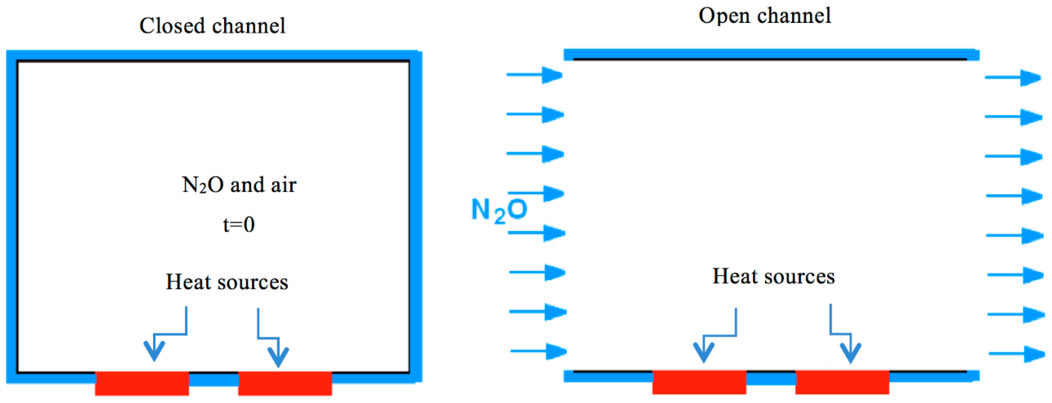
• In the bottom plates, there are two heat sources (or hot spots) for both the opened and closed channels at a higher temperature than the low constant temperature set in 7. These heat sources trigger the (N₂O decomposition) reaction.
• The concentrations of chemical species are kept sufficiently small so that they dominate the properties of air during the phenomenon of natural convection.

There are experimental values for the kinetic constants k₁ and k₂ in (10), which we assume follow the Arrhenius law [30].

$$k_1={10}^{19.39}{e}^{-81800/RT}$$

(15)

$$k_2={10}^{8.69}{e}^{-28400/RT}$$

(16)

We chose temperatures in order that the chemical reaction rate is relatively slow so the heat generated by it is also small.

3. The Lattice Botlzmann Model

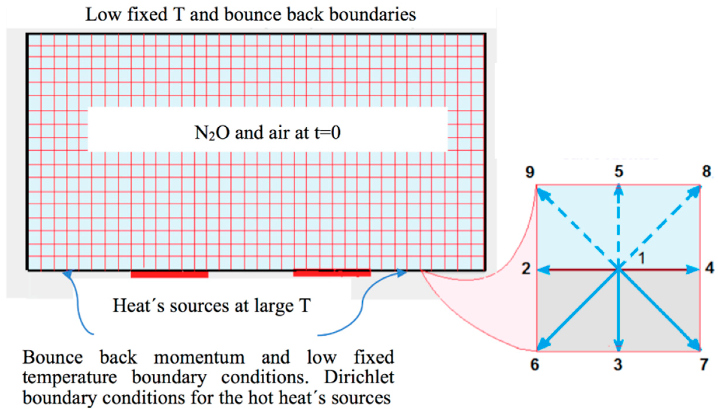
In this section, we introduce the general lattice Boltzmann framework used in this paper.

3.1. Open Channel

As mentioned above, three lattice Boltzmann structures are used in this paper. The first one concerns the thermo-hydrodynamics issue. We proposed for the momentum distribution function the following equation:

$$f_i\left(x+c_i\nabla t,t+\nabla t\right)-f_i\left(x,t\right)=-\frac{\Delta t}{{\tau }_F}\left[f_i\left(x,t\right)-f_i^{eq}\left(x,t\right)\right]+J_i$$

(17)

For J_i, the buoyant term, we use the Boussinesq approximation, namely

$$J_i=3w_i{g}_y\beta \cdot \left[T\left(x,t\right)-T_{\infty }\right]\cdot \rho \left(x,t\right)\cdot c_{iy}$$

(18)

A second LBE is formulated for the temperature field. The equation for the thermal distribution function is:

$$g_i\left(x+c_i\Delta t,t+\Delta t\right)-g_i\left(x,t\right)=-\frac{\Delta t}{{\tau }_T}\left[g_i\left(x,t\right)-g_i^{eq}\left(x,t\right)\right]$$

(19)

A third LBE is formulated for the chemical reaction kinetics that rules the species’ concentration evolution.

$$h_i^{\alpha }\left(x+c_i\Delta t,t+\Delta t\right)-h_i^{\alpha }\left(x,t\right)=-\frac{\Delta t}{{\tau }_D}\left[h_i^{\alpha }\left(x,t\right)-h_i^{\alpha ,eq}\left(x,t\right)\right]+\frac{\Delta t}{Q}{R}_Q$$

(20)

here, τ_D is the diffusion relaxation time ${\tau }_D=\frac{D_{\alpha }}{c_s^2}+\frac{1}{2}$, being D_α the α’s chemical specie Fick diffusion coefficient. The corresponding (three LBE) distribution equilibrium functions are defined by the following equations:

$$f_i^{eq}\left(x,t\right)=w_t\rho \left[1+\frac{c_{iA}{u}_A}{c_s^2}+\frac{u_A{u}_B}{2c_s^2}\left(\frac{c_{iA}{c}_{iB}}{c_s^2}-{\delta }_{AB}\right)\right],$$

(21)

$$g_i^{eq}\left(x,t\right)=w_{t}T\left[1+\frac{c_{iA}{u}_A}{c_s^2}+\frac{u_A{u}_B}{2c_s^2}\left(\frac{c_{iA}{c}_{iB}}{c_s^2}-{\delta }_{AB}\right)\right],$$

(22)

$$h_i^{\alpha ,eq}\left(x,t\right)=w_{\alpha }{c}_i\left[1+\frac{c_i^{\alpha }\cdot u}{c_s^2}+\frac{{\left(c_i^{\alpha }\cdot u\right)}^2}{2c_s^4}-\frac{u^2}{2c_s^2}\right].$$

(23)

In a reactive system, we have as many equations ((20) and (23)) as needed (the same number as the chemical species involved in the reactions). The macroscopic variables are obtained as usual in the LBM. For example, the different species´ concentrations are obtained from the mesoscopic distribution functions as follows:

$$C_{\alpha }={\displaystyle \sum _i{h}_i^{\alpha }}.$$

(24)

In Figure 2, we schematically introduce the so-called open channel system. The N₂O current (mixed with air) enters by the open rectangular channel on the left side with a fixed and uniform speed and laminar regime (low Reynolds numbers). The internal part the channel interacts with heat sources which triggers the N₂O thermal decomposition, following the mechanism’s reaction proposed in this paper by Equations (13) and (14). Simultaneously, the very same heat sources cause the appearance of convection rolls, and the reaction evolves at different rates, depending on the local temperature achieved by the reactive molecules in the fluid at each site of the channel.

As for the boundary conditions we set the following scheme in the open channel case:

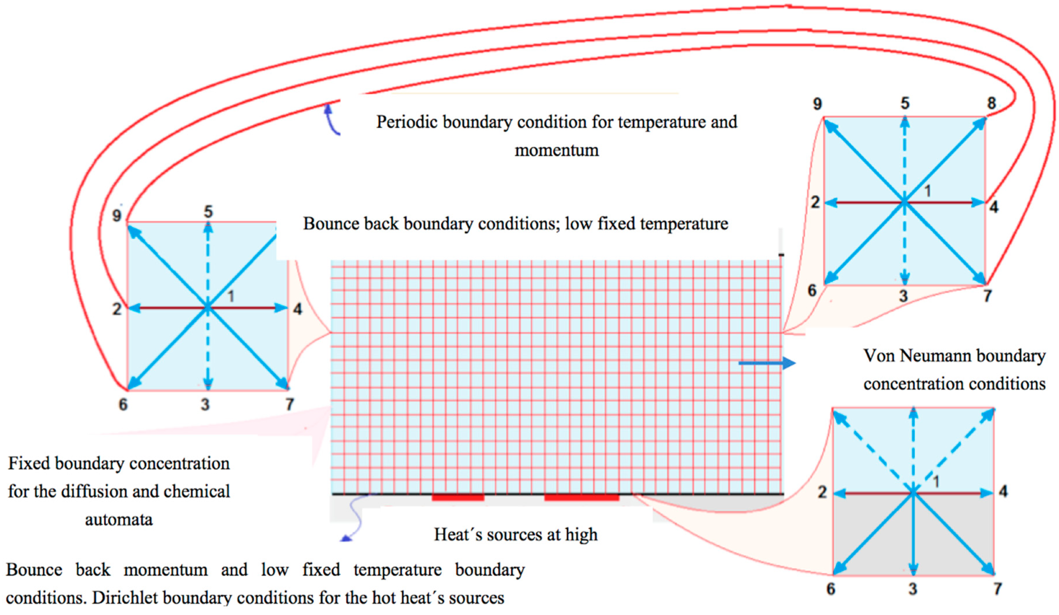
• For the top plate, bounce back boundary conditions for the fluid dynamic LBE and a low constant isothermal boundary conditions for the thermic LBE are used.
• Inlet and outlet periodic boundary conditions, for the moment and thermal LBE, are set.
• For the bottom plate, bounce back boundary conditions are imposed in all the nodes for the hydrodynamic LBE, while for thermal LBE we used bounce back conditions as well, except in the heat sources sites where Dirichlet boundary conditions are set.

After obtaining the profiles of velocity and temperature in steady-state, we assess the evolution of the concentration of the chemical species for the reactive diffusional LBE. This procedure results from the fact that kinetics is coupled with the temperature field through the Arrhenius law, namely the concentration rate changes due to kinetic law by both concentration and temperature fields.

These boundary conditions are:

• Top and bottom bounce back boundary conditions.
• Invariable concentration in the inlet of the channel.
• Null gradient concentration in the outlet of the channel (von Neumann condition).

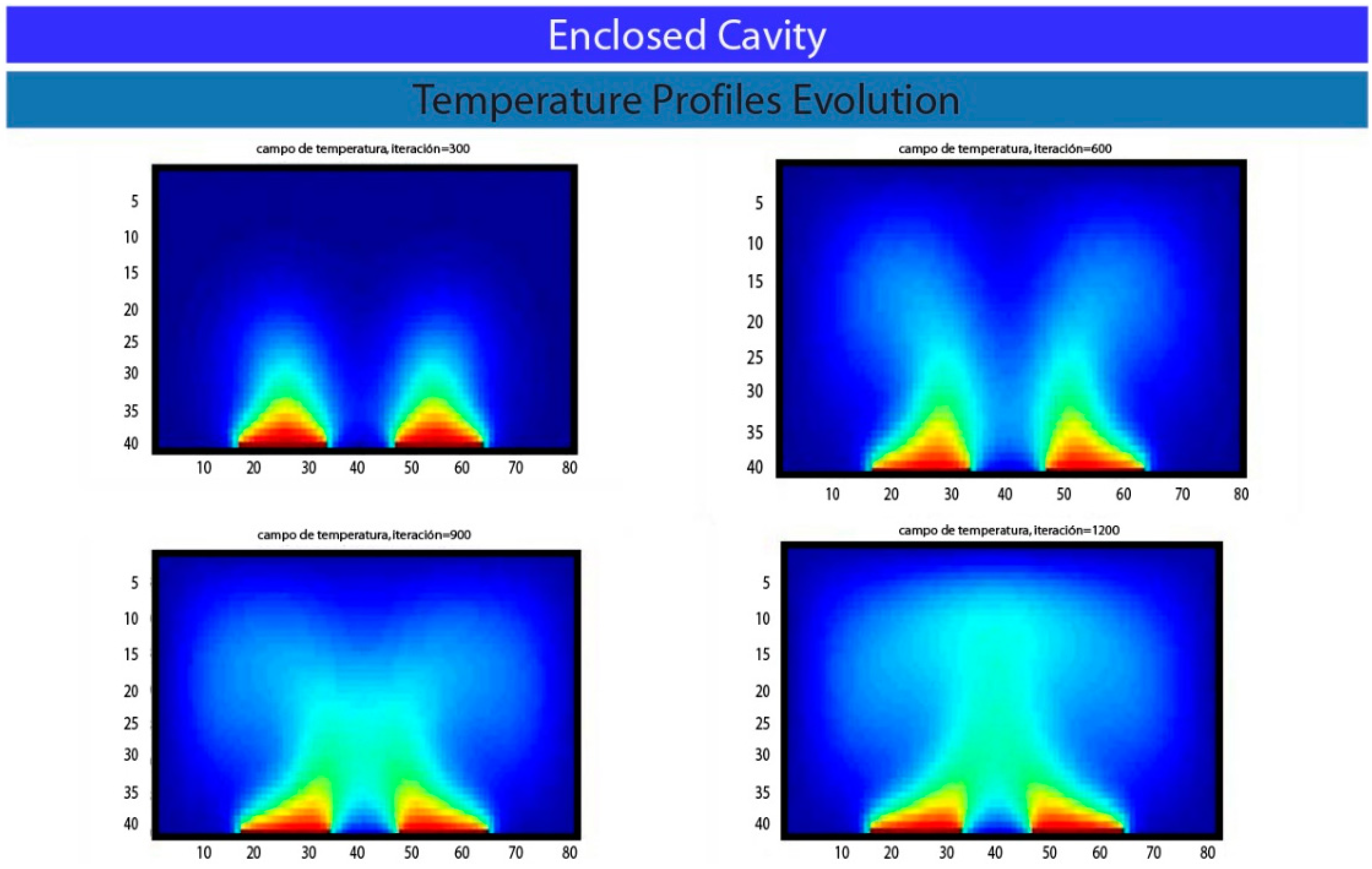
Figure 2. The lattice Boltzmann model for a reactive flow (a mixture of nitrous oxide and air), with heat sources that promote its thermal decomposition in an open channel.

Figure 2. The lattice Boltzmann model for a reactive flow (a mixture of nitrous oxide and air), with heat sources that promote its thermal decomposition in an open channel.

3.2. Closed Channel

Now consider nitrous oxide initially confined to a vessel at 250 K and suddenly the sources located in the bottom plate rise their temperature to 300 K (by the hot spots) producing the thermal decomposition of the laughing gas (Rayleigh–Bénard flow). All the settings given by the open channel case are kept except for the boundary conditions. In the closed channel case, these are the following:

• Bounce back boundary conditions at all the sites for the fluid and thermal LBE on all borders, except at the heat’s sources.
• Diritchlet boundary conditions at all high temperature sites (heat sources).
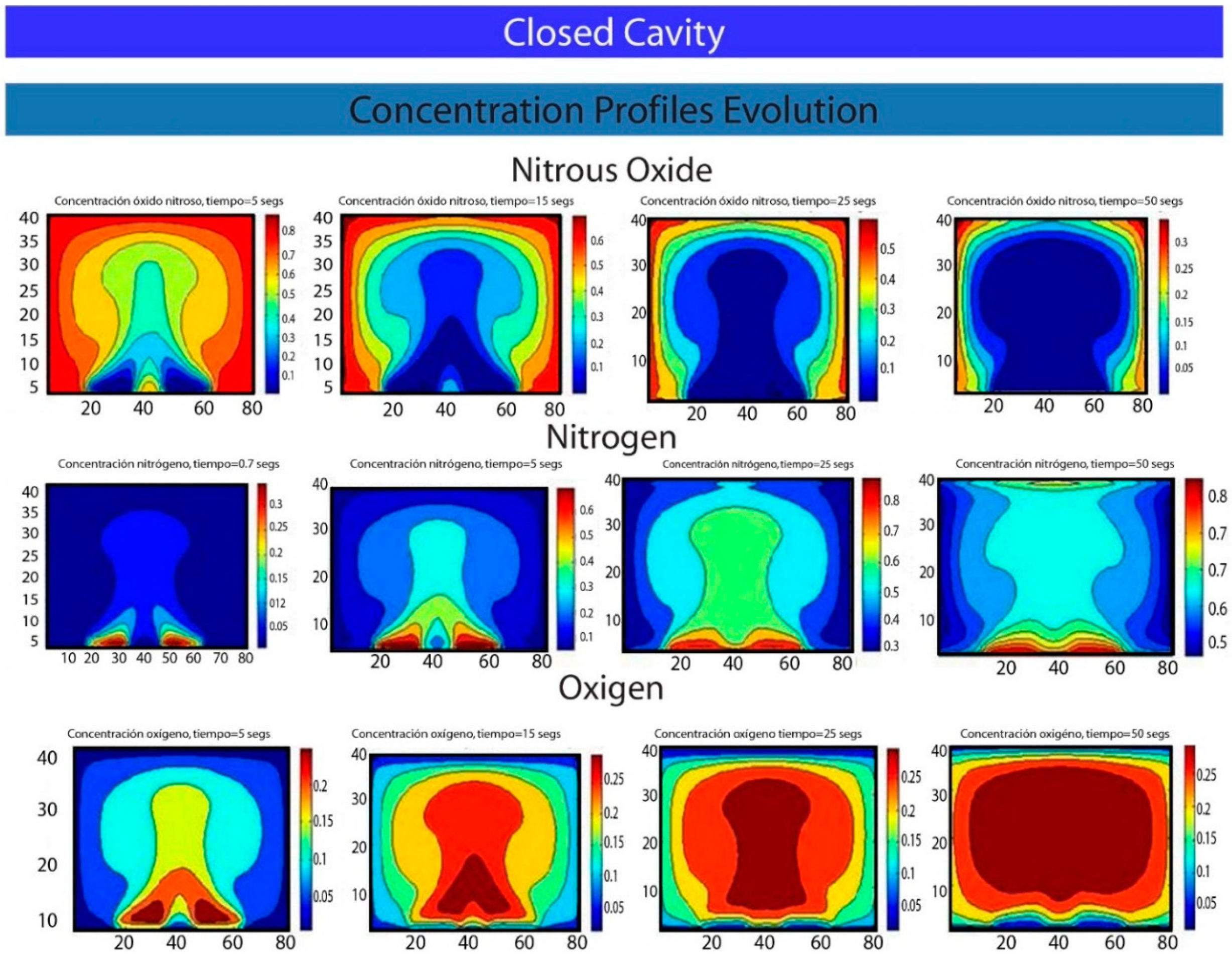
• Initial state with uniformly distributed nitrous oxide in the closed vessel, with initial concentration C₀ and initial temperature T₀, smaller than the temperature of the sources.
• Bounce back boundary conditions at all the sites for the reaction-diffusion LBE on all borders.

Figure 3 is a schematic representation of this system.

Figure 3. The lattice Boltzmann model for a reactive flow containing nitrous oxide mixed with air, with heat sources that promote its thermal decomposition in a closed vessel.

Figure 3. The lattice Boltzmann model for a reactive flow containing nitrous oxide mixed with air, with heat sources that promote its thermal decomposition in a closed vessel.

4. The Lattice Botlzmann Algorithm

In the following we describe the LBM algorithm used in this paper to perform the simulation of our models that allowed us to obtain our results.

4.1. Open Channel

After the discretization of the rectangular 2D domain, a D2Q9 lattice is implemented and then the following standard LBM steps are applied:

• The distribution functions f and g for the velocity u and temperature T fields, respectively, were evaluated simultaneously in a coupled fashion, taking into account iterative calculations performed by the following steps:

  1.1

  Propagation (streaming) of the f and g distribution functions.

  1.2

  Calculation of the distribution functions at equilibrium; f_eq and g_eq.

  1.3

  Actualization of the f and g distribution functions.

  1.4

  Introduction of thermal and fluid dynamics boundary conditions.

  1.5

  Calculation of the u and T fields from the new f and g distribution functions.

  1.6

  Assessment of the new and preceding values of u and T, if they are closed enough, finish the iterations; else, return to step 1.1.

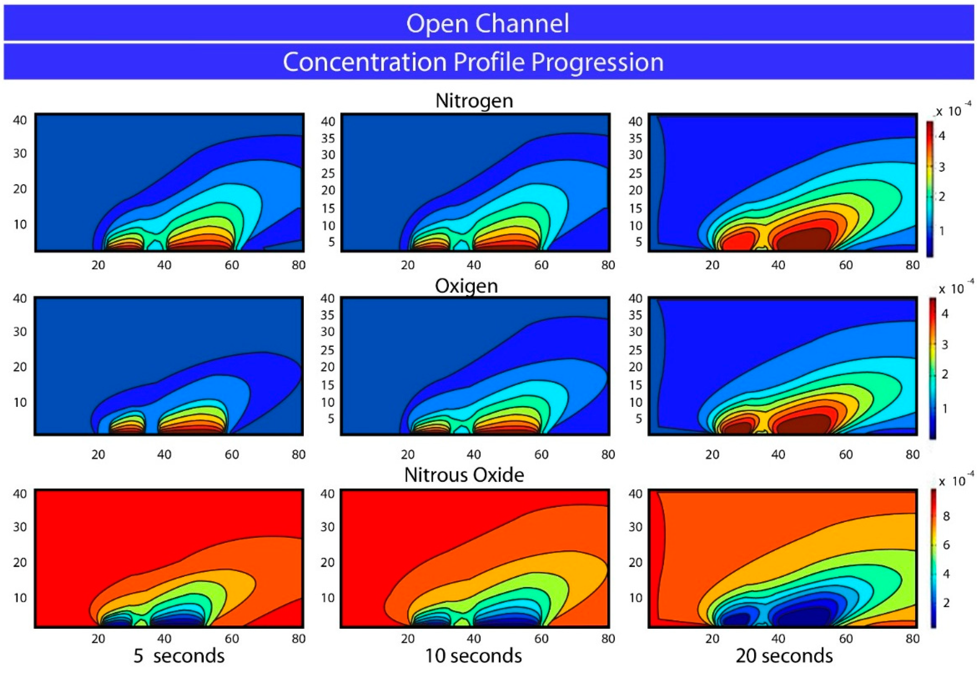
• Once obtaining the steady temperature and velocity profiles, the temporal evolution of the distribution functions h_i for each one of the three chemical species is calculated, solving the LBM equations for the reaction-diffusion advection phenomena. This is a non-iterative procedure, structured practically by the same steps as the ones in the thermo-hydrodynamic analysis, except for that in the formulation of the diffusional distribution functions for each chemical species. The chemical kinetics term (Arrhenius law also considered) is introduced, keeping the 1:1:1/2 stoichiometric relationships between reactants and products.

After a short period of time, the concentrations of the three chemical species reach a steady-state, due to the constant in-and-out reagent.

4.2. Closed Channel

In this case, we use the open channel algorithm modifying a few instructions in the algorithm concerning the new boundary conditions and establishing a speed equal to zero in the input stream. The remaining instructions are kept unchanged in the algorithm.

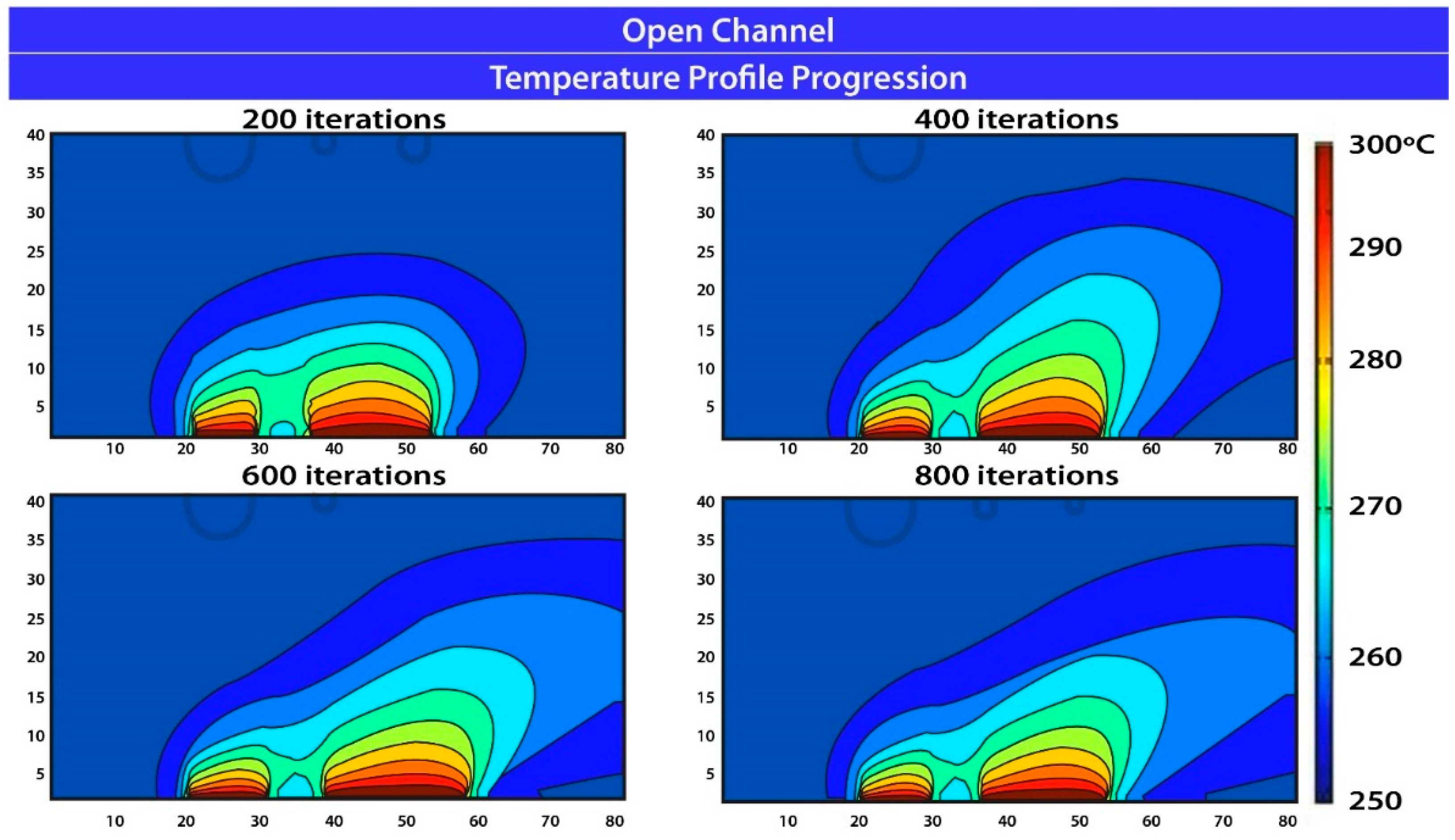
5. Results and Conclusions

The results of our calculations are presented in Figure 4 and Figure 5 for the open channel and in Figure 6 and Figure 7 for the closed channel.

One goal of this paper is the analysis of the chemical reactions’ dynamics that are carried out on systems presenting thermo-hydrodynamic instabilities, using Boussinesq approximation since this is considered a main stream topic. The study presented here is a new step towards this direction. The model presented in this paper includes a non-stationary thermo-hydrodynamic system where the heat generated by the chemical reactions has an important role in the temperature interval studied. The reaction enthalpy data of several chemical reactions are available in the literature and can be plugged into the algorithm. The heat generated would lead to a different evolution of the Bénard convection rolls. In this case, the solution of the Boussinesq approach and the associated coupled chemical is quite different and shall be addressed elsewhere.

Finally, data numerical analysis can be performed by Fourier series on the bidimensional images (or rough data on the plane) providing precise functions from the contours depicted in Figure 4, Figure 5, Figure 6 and Figure 7. For example, in Figure 5, for the Nitrogen produced after 5 s, the upper contour of the lowest and second lowest concentration areas can be approached by the following function; $y=-204+166.71\cos \left(.0034x\right)+361.2\sin \left(.0034x\right)$ with a correlation of 0.994, being x and y space coordinates in the channel. Further work should be done in the near future to take full advantage of our approach.

Figure 4. Temperature field evolution for the Bernard–Poiseuille reactive flow as iterations are carried on up to reach the thermo-hydrodynamic steady state.

Figure 4. Temperature field evolution for the Bernard–Poiseuille reactive flow as iterations are carried on up to reach the thermo-hydrodynamic steady state.

Figure 5. Species concentration field evolution for the Bénard–Poiseuille reactive flow as iterations that are carried out for 5, 10 and 20 s.

Figure 5. Species concentration field evolution for the Bénard–Poiseuille reactive flow as iterations that are carried out for 5, 10 and 20 s.

Figure 6. Temperature field evolution for the Rayleigh–Bénard reactive flow as iterations that are carried out to reach the thermo-hydrodynamic steady state, x and y are the space coordinates in the cavity.

Figure 6. Temperature field evolution for the Rayleigh–Bénard reactive flow as iterations that are carried out to reach the thermo-hydrodynamic steady state, x and y are the space coordinates in the cavity.

Figure 7. Species concentration field evolution for the Rayleigh–Bénard reactive flow as iterations that are carried out for 5, 15, 25 and 50 seconds, here x and y are the space coordinates in the cavity.

Figure 7. Species concentration field evolution for the Rayleigh–Bénard reactive flow as iterations that are carried out for 5, 15, 25 and 50 seconds, here x and y are the space coordinates in the cavity.

References

1. Dragani, W.C. A feature model of surface pressure and wind fields associated with passage of atmospheric cold fronts. Comp. Geosci. 1999, 25, 1149–1157. [Google Scholar] [CrossRef]
2. Agee, E.M. Mesoscale cellular convection over the oceans. Dyn. Atmos. Oceans 1987, 10, 317–341. [Google Scholar] [CrossRef]
3. Nicolas, X. Revue bibliographique sur les écoulements de Poiseuille–Rayleigh–Bénard: écoulements de convection mixte en conduites rectangulaires horizontales chauffées par le bas. Int. J. Therm. Sci. 2002, 41, 961–1016. [Google Scholar] [CrossRef]
4. Bograchev, D.A.; Davidov, A.D.; Volgin, V.M. Linear stability of Rayleigh–Benard–Posieuille convection for electrochemical system. Int. J. Heat Mass Transf. 2008, 51, 4886–4891. [Google Scholar] [CrossRef]
5. Kakuda, K.; Miura, S. Finite element simulation of three- dimensional Rayleigh–Bénard convection. Int. J. Comput. Fluid Dyn. 2001, 15. [Google Scholar] [CrossRef]
6. Murty, V.D. A numerical investigation of Benard convection using finite elements. Comp. Fluids 1986, 14, 379–391. [Google Scholar] [CrossRef]
7. Lan, C.H.; Ezekoye, O.A.; Howell, J.R.; Ball, K.S. Stability analysis for three-dimensional Rayleigh–Bénard convection with radioactively participating medium using spectral methods. Int. J. Heat Mass Transf. 2003, 46, 1371–1383. [Google Scholar] [CrossRef]
8. Howle, L.E. A comparison of the reduced galerkin and pseudo-spectral methods for simulation of steady Rayleigh–Bénard convection. Int. J. Heat Mass Transf. 1996, 39, 2401–2407. [Google Scholar] [CrossRef]
9. Luo, X.; Chen, W.-K. A discussion on finite-difference schemes for low Prandtl number Rayleigh–Bénard convection. In Advanced Computational Methods in Heat Transfer; Sundén, B., Brebbia, C.A., Eds.; WIT Press: Ashurst, UK, 1994. [Google Scholar]
10. Park, H.M.; Ryu, D.H. Rayleigh–Bènard convection of viscoelastic fluids in finite domains. J. Non-Newton. Fluid Mech. 2001, 98, 169–184. [Google Scholar] [CrossRef]
11. Tzeng, P.-Y.; Liu, M.-H. Direct-simulation Monte Carlo modeling on two-dimensional Rayleigh–Bénard instabilities of rarefied gas. Numer. Heat Transf. A Appl. 2005, 47, 805–823. [Google Scholar] [CrossRef]
12. Zhang, J.; Fan, J. Kinetic study of the Rayleigh–Bénard flows. Chin. Sci. Bull. 2009, 54, 364–368. [Google Scholar] [CrossRef]
13. Higuera, F.J.; Succi, S. Simulating the flow around a circular cylinder with a Lattice Boltzmann equation. Europhys. Lett. 1989, 8, 517–521. [Google Scholar] [CrossRef]
14. Benzi, R.; Succi, S.; Vergassola, M. The lattice Boltzmann equation: theory and applications. Phys. Rep. 1992, 222, 145–197. [Google Scholar] [CrossRef]
15. Shan, X.W. Simulation of Rayleigh–Bénard convection using a lattice Boltzmann method. Phys. Rev. E 1997, 55, 2780–2788. [Google Scholar] [CrossRef]
16. Kao, P.-H.; Yang, R.-J. Simulating oscillatory flow in Rayleigh–Bénard convection using the lattice Boltzmann method. Int. J. Heat Mass Trans. 2007, 50, 3315–3328. [Google Scholar] [CrossRef]
17. Barrios, G.; Rechtman, R.; Rojas, J.; Tovar, R. The lattice Boltzmann equation for natural convection in a two-dimensional cavity with a partially heated wall. J. Fluid Mech. 2005, 522, 91–100. [Google Scholar] [CrossRef]
18. Chandrasekar, S. Hydrodynamic and Hydromagnetic Stabilities; Clarendon Press: Oxford, UK, 1961. [Google Scholar]
19. Massaioli, F.; Benzi, R.; Succi, S. Exponential tails in 2-dimensional Rayleight–Bérnard convection. Europhys. Lett. 1993, 21, 305–310. [Google Scholar] [CrossRef]
20. Benzi, R.; Tripiccione, R.; Massaioli, F.; Succi, S.; Ciliberto, S. On the scaling of the velocity and temperature structure functions in Rayleigh–Bénard convection. Europhys. Lett. 1994, 25, 341–346. [Google Scholar] [CrossRef]
21. Moussaoui, M.A.; Jami, M.; Mezrhab, A.; Naji, H. Lattice Boltzmann simulation of convective heat transfer from heated blocks in a horizontal channel. Numer. Heat Transf. A Appl. 2009, 56, 422–443. [Google Scholar] [CrossRef]
22. Amaya-Ventura, G.; Rodríguez-Romo, S. 2D Lattice Boltzmann Simulation of Chemical Reactions within Rayleigh–Bénard and Poiseuille–Bénard Convection Systems. In Proceedings of the International Conference on Numerical Analysis and Applied Mathematics 2011 (ICNAAM 2011), Halkidiki, Greece, 19–25 September 2011; pp. 1798–1801.
23. Chen, S.Y.; Doolen, G.D. Lattice Boltzmann method for fluid flows. Annu. Rev. Fluid Mech. 1998, 30, 329–364. [Google Scholar] [CrossRef]
24. He, X.Y.; Chen, S.Y.; Doolen, G.D. A novel thermal model for the lattice Boltzmann method in incompressible limit. J. Comput. Phys. 1998, 146, 282–300. [Google Scholar] [CrossRef]
25. Zhang, L.; Wang, M. Modeling of electrokinetic reactive transport in micropore using a coupled lattice Boltzmann method. J. Geophys. Res. Solid Earth 2015, 120, 2877–2890. [Google Scholar] [CrossRef]
26. Yamamoto, K.; He, X.Y.; Doolen, G.D. Simulation of combustion field with lattice Boltzmann method. J. Stat. Phys. 2002, 107, 367–383. [Google Scholar] [CrossRef]
27. Chiavazzo, E.; Karlin, I.V.; Gorban, A.N.; Boulouchos, K. Coupling of the model reduction technique with the lattice Boltzmann method for combustion simulations. Combust. Flame 2010, 157, 1833–1849. [Google Scholar] [CrossRef]
28. Chiavazzo, E.; Karlin, I.V.; Gorban, A.N.; Boulouchos, K. Efficient simulations of detailed combustion fields via the lattice Boltzmann method. Int. J. Numer. Methods Heat Fluid Flow 2011, 21, 494–517. [Google Scholar]
29. Charru, F. Hydrodynamic Instabilities, 1st ed.; Cambridge University Press: Cambridge, UK, 2011. [Google Scholar]
30. Levenspiel, O. Ingeniería de las Reacciones Químicas; Reverté: Barcelona, Spain, 1987. (In Spanish) [Google Scholar]