The Character of Entropy Production in Rayleigh–Bénard Convection

1
College of architecture and Environment, Sichuan University, Chengdu 610065, China
2
Sichuan College of Architectural Technology, Deyang 618000, China
*
Author to whom correspondence should be addressed.
Entropy 2014, 16(9), 4960-4973; https://doi.org/10.3390/e16094960
Submission received: 23 June 2014
/
Revised: 20 August 2014
/
Accepted: 12 September 2014
/
Published: 17 September 2014
Abstract
:In this study; the Rayleigh–Bénard convection model was established; and a great number of Bénard cells with different numbered vortexes were acquired by numerical simulation. Additionally; the Bénard cell with two vortexes; which appeared in the steady Bénard fluid with a different Rayleigh number (abbreviated Ra); was found to display the primary characteristics of the system’s entropy production. It was found that two entropy productions; which are calculated using either linear theory or classical thermodynamic theory; are all basically consistent when the system can form a steady Bénard flow in the proper range of the Rayleigh number’s parameters. Furthermore; in a steady Bénard flow; the entropy productions of the system increase alongside the Ra parameters. It was also found that the difference between the two entropy productions is the driving force to drive the system to a steady state. Otherwise; through the distribution of the local entropy production of the Bénard cell; two vortexes are clearly located where there is minimum local entropy production and in the borders around the cell’s areas of larger local entropy production.
1. Introduction
As is commonly understood, macroscopic convection occurs when a thin layer of fluid, in a static state, is evenly heated from the bottom, causing its temperature gradient to exceed a certain value. Looking down at the surface of the fluid, a number of hexagonal vortexes appear, resembling a beehive. This phenomenon was first observed by Bénard in his experiment in 1901, thus, the beehive-like vortexes are named “Bénard cells”, after him.
In 1916, Rayleigh created a working description of the Bénard convection phenomenon in theory. After him, many other studies have been carried out on the subject of Rayleigh–Bénard convection. Several experts and academics have made valuable finds in this field of study, not only regarding the theory itself, but its practical applications in engineering. When discussing the theoretical aspect, studies typically focus on flow stability transformation [1,2], (from laminar flow to turbulence,) convection state in turbulence [3,4], qualification of the convection’s appearance [5–7], the varying number of Bénard cell vortexes according to the Rayleigh number (Ra) [8,9], and so on. In engineering applications, primary achievements in the field involve the following areas: nuclear magnetic resonance pulsed-field-gradient diffusion measurements [10], the security of liquefied natural gas packets [11], weather forecast systems [12], freeze soil roadbeds [13], mantle convection [14] and Rayleigh–Bénard convection in reservoirs, lakes and oceans [15–17].
As one of the models in a force-driven system in the context of non-equilibrium thermodynamics, the Bénard system is driven by the temperature difference between the upper and the lower surface of the fluid. The Bénard convection model is a typical model of non-linearity phenomenon in a dissipation system, and most research on the subject remains theoretical. Robert K. Niven [18] proved that steady-state flow of an incompressible fluid in parallel pipes can simultaneously satisfy two contradictory extremum principles in the entropy production, depending on the flow conditions. For a constant total flow rate, the flow can satisfy (i) a pipe network minimum entropy production (MinEP) principle with respect to the flow rates and (ii) the maximum entropy production (MaxEP) principle of Ziegler and Paltridge with respect to the choice of flow regime. Yohei Kawazura and Zensho Yoshida [19] studied two different types of self-organizing and sustaining ordered motion in fluids or plasmas—one is a Bénard convection (or streamer) and the other is a zonal flow. They have compared the two types by introducing a thermodynamic phenomenological model and evaluated the corresponding entropy production rates (EP). It was found that the parallel (series)-connection system tends to minimize (maximize) the total EP when a constant-current power supply drives the system, and this minimum/maximum relation flips when a constant-voltage power supply is connected. However, a few studies on the characteristics of the system’s entropy production, especially on the topic of how entropy production acts on Rayleigh–Bénard flow, do exist.
This study will create basic theoretical research on the characteristics of the Rayleigh–Bénard convection system’s entropy production. In this research, the Rayleigh–Bénard convection model was established, and a great number of Bénard cells with different numbered vortexes were acquired by numerical simulation. The two entropy productions of the system were calculated using either linear theory or classical thermodynamic theory. By studying the entropy productions in a Rayleigh–Bénard system, some results were obtained. The two entropy productions of the system are all basically consistent when the system can form a steady Bénard flow in the proper range of the Ra number’s parameters. Furthermore, in a steady Bénard flow, the entropy productions of the system increase alongside the Ra parameters. It was also found in this research that the difference between the two entropy productions is the driving force to drive the system to a more complex state. Otherwise, through the distribution of the local entropy production of the Bénard cell, two vortexes are clearly located where there is minimum local entropy production and in the borders around the cell’s areas of larger local entropy production. The research also intends for these results to assist in the development and perfection of Bénard convection and to provide additional information relevant to the study of far from equilibrium thermodynamics.
2. Model Establishment
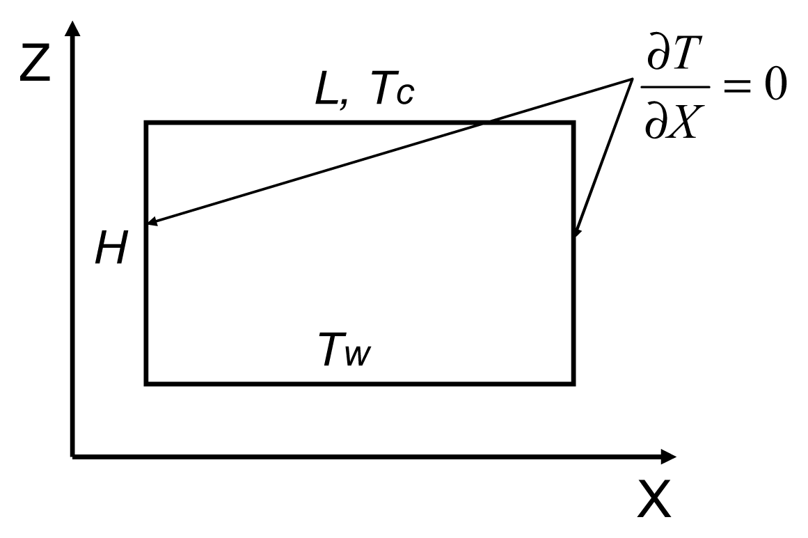
The physical model of Rayleigh–Bénard convection in this research is shown in Figure 1. At a height of H and a width of L, the incompressible Newtonian fluid is full of a rectangular pocket. The fluid’s physical properties have known value, and they meet the Boussinesq hypothesis. The rectangular pocket is evenly heated from the bottom, and both sides of the rectangular pocket are adiabatic. The temperature of the fluid’s lower surface is Tw; the upper surface is Tc. The temperature difference between the upper and the lower surface of the fluid is very important for this experiment. When the temperature difference is in a certain range, Bénard convection will occur in the flow. This research is developed based on such a situation, which has been mentioned above. Due to the rectangular pocket’s length in the flow direction having no effect on the result of this research, therefore, only the two-dimensional case will be considered in order to simplify the model.
In the subject of this study, the center mesh system and the finite volume method were used to disperse the control equations; the SIMPLE method was used to solve the equations, and the computer language FORTRAN was applied in the programming. The staggered mesh used in the simulation is represented in Figure 2. In the staggered mesh, the pressure difference between the two adjacent nodes is the natural driving force of the velocity component. The HSMAC algorithm was used for the coupling of velocity and pressure. The sinusoidal function was used for mesh segmentation, and the non-uniform mesh is shown in Figure 3.
For a deterministic system, the motion of all of the particles is governed by a set of differential equations. The dimensionless equations describe thermal convection in the Rayleigh–Bénard model, shown here:
In the dimensionless equations, X, Z represent the two directions in Cartesian coordinates. Vn (n = x, y, z) represent the velocity components. Θ represents the temperature. Gr, known as the Grashof number, is the buoyancy and viscous force ratio. Moreover,
, named the Prandtl number, represents the relationship between the thermal properties and convective heat transfer. There, ν is the kinematics viscosity and K is the thermal diffusivity. In this research, the Pr has a fixed value as 6.7. Ra is also a dimensionless quantity, called the Rayleigh number, which is closely related to Pr and Gr.
In Equation (5)Tw is the lower surface’s temperature, Tc is the upper surface’s temperature, h is the distance between the upper and the lower surface, α is the thermal expansion coefficient of the fluid, g is the gravitational acceleration, K is the thermal diffusion coefficient, ν is the kinematics viscosity coefficient and β is the fluid temperature’s gradient in the vertical direction. It can be calculated by using Equation (6).
Boundary conditions:
- In the upper boundary: Vz = 0, Vx = 0, T = 0
- In the lower boundary: Vz = 0, Vx = 0, T = 1
Additionally, on both sides of the wall: Vz = 0, Vx = 0,
3. Calculation of Entropy Production
In order to explore the characteristics of entropy production in a Bénard convection system with non-equilibrium thermodynamics, the entropy production of the system must be calculated first. There are two ways to do this. One is to employ classical thermodynamics theory in order to calculate the entropy production value, recorded as Sp. Another way is by using the linear non-equilibrium thermodynamic theory, which also records the entropy production value as Sg. The values for the two entropy productions are not always consistent with each other, however, because the state of the system changes. Only in a non-equilibrium thermodynamic linear zone system are the two entropy productions consistent. The entropy productions Sp and Sg in the Bénard system, using a variety of methods, were obtained in this study under different operation conditions. Through comparing the calculation results, the characteristics of the Bénard system that deviate from the linear area were acquired and analyzed.
3.1. Entropy Production Sp Based on Classical Thermodynamics
In this research, the Bénard convective system is in a non-equilibrium steady state. The primary characteristic of a non-equilibrium steady state is the change in entropy to zero, recorded as ΔS = 0. The entropy change of the system includes two parts: the flow of entropy Sf, which is supplied externally, and entropy production Sp, which is produced irreversibly and from within the system. This is expressed by the well-known entropy balance formula, ΔS = Sf + SP.
By using the entropy balance equation, one can see that when the system entropy is zero, the entropy production of the system is equal to the negative entropy flow. For that reason, the method for calculating the entropy production Sp is greatly simplified. Only the negative entropy flow needs to be calculated. The flow of entropy may take positive or negative values. In this model, the influx entropy flow of the system is defined as positive, and the outflow is defined as negative. The flow of entropy is composed of mass flow and heat flow, which reads:
In Equation (7)Sfq is heat flow and Sfm is mass flow. In a Bénard system, only the value for heat flow is needed to calculate the flow of entropy, because there is no mass flow in the system. The heat entropy flow of the system Sfq is the difference between the inflow and the outflow from the boundary. Both sides of the wall in the model (Figure 1) are thermally insulated, so the heat entropy flow of the system Sfq is the difference between the inflow from surface and the outflow from the bottom.
Based on classical thermodynamics, the formulation of entropy production Sp is expressed as Equation (8).
In Equation (8), Γ is the boundary and Q is heat flow. In this system, the inflow is positive and the outflow is negative.
3.2. Entropy Production Sg Based on the Linear Non-Equilibrium Thermodynamic
In linear non-equilibrium thermodynamics, the entropy production rate (local entropy production) is calculated by Equation (9). Equation (9) is the well-known formula expression of the linear thermodynamic law.
In Equation (9), the first item on behalf of the entropy production rate is caused by a chemical reaction; the second item is caused by heat conduction; the third item is caused by diffusion; and the rest of the three items are caused by viscosity. In the Rayleigh–Bénard model, there is no chemical reaction and diffusion. For incompressible and isotropic fluid, there is pνxν = 0 and
.
By using linear non-equilibrium thermodynamics combined with the actual situation presented in this study, the calculation formula for the entropy production rate (local entropy production) is expressed as Equation (10) [20].
In Equation (10)Jq is the thermodynamic flux and Xq is thermodynamic force.
is the symmetrical part of the viscous pressure tensor with trace zero.
is the viscous force tensor.
and
are conjugate, and they cause the viscosity together. η is the shear viscosity coefficient. It is equal to the fluid movement viscosity coefficient in this model. λ is the heat conductivity coefficient and was defined as 0.1 in this research.
The system’s total entropy production Sg is obtained by using the global integral of the entropy production rate.
in which Ω is the whole computational domain.
4. Bénard Cell Pattern
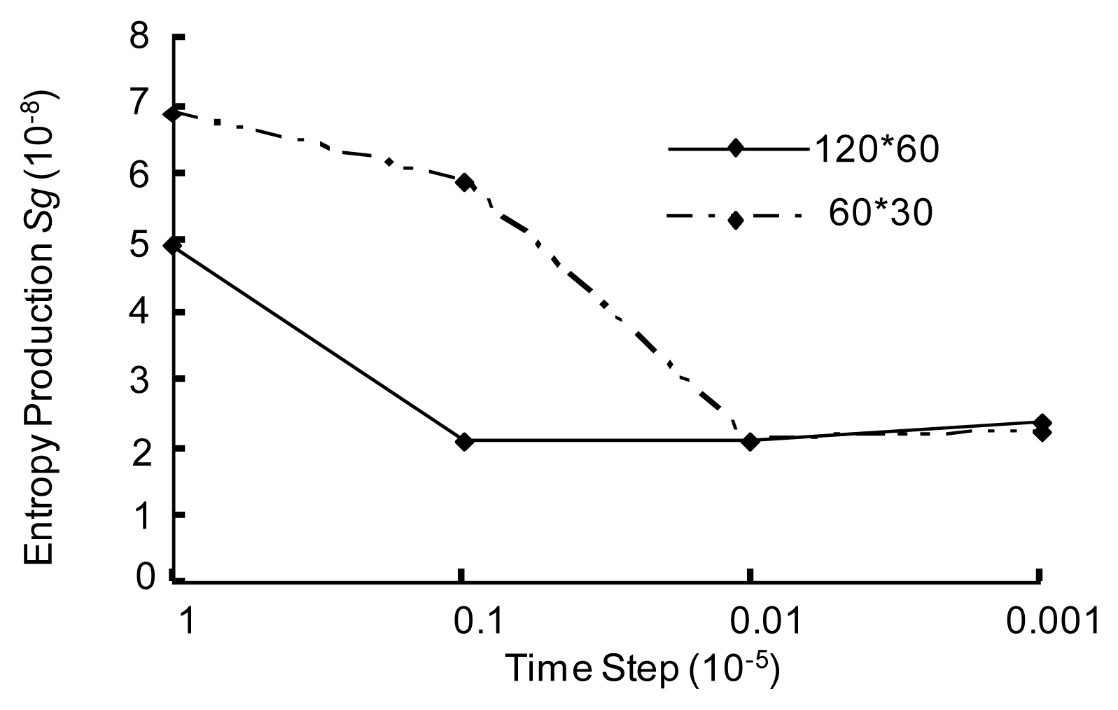
In this study, different operation conditions can be actualized by changing the aspect ratio of L/H in the model or in the dimensionless parameter Ra. In the numerical simulation, program, mesh and the time step were all controlled for accuracy. The mesh size or time step effect on the result of the entropy production, Sg, can be seen in Figure 4. In Figure 4, there are two sets of entropy production, where mesh cells had time steps of 120 by 60 and 60 by 30 in size, respectively. There is a significant difference in the two entropy productions in different mesh sizes when the time step is bigger than 10−6; but, there is no obvious difference when the time step is smaller than 10−7; thus, we conclude that the mesh sizes have little effect on the result of entropy productions when the time step is smaller than 10−7.
The smaller the mesh size is, the slower the simulation runs. Therefore, in the numerical simulation, we used a mesh size of 60 by 30 to optimize the results. From Figure 4, it is clear that there is a slight difference in entropy production when the mesh size in the simulation was 60 by 30 and the time step was 10−7 or smaller. In order to reduce the amount of calculations needed, the time step was set to 10−7. For ease of calculation and to account for situational changes in the flow field, a time step of 10−7 and a mesh size of 60 by 30 were used as a control, to optimize the results of this study.
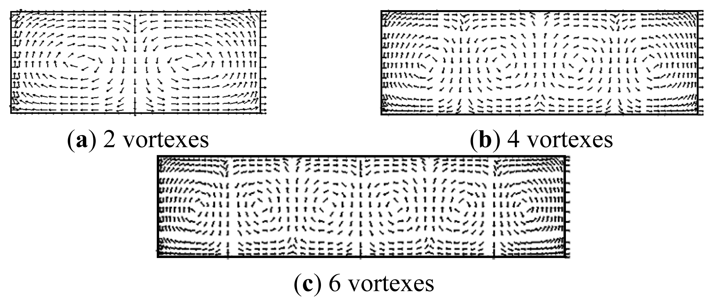
Figure 5 shows some Bénard cells with different numbers of vortexes, which were obtained by numerical simulations. Some steady Bénard flow states under different parameters were also obtained. In the process of the simulation, researchers found that the value of Ra plays a very important role of reaching a steady state in the flow. The model’s aspect ratio L/H has a significant influence on the number of vortexes of Bénard cells that appear on the flow section. For example, the number of vortexes in the Bénard cells was 2, 4, 6, when L/H = 2,3,4, and the flow fields were in a steady state. In the case of certain L/H values, as long as the Bénard flow was formed, the system reached stability eventually. After some time, the macro cell pattern observed in a steady flow did not change. In this paper, a series of research results, Ra ranges between 100,50 and 78,725, L/H = 2 were used to explore the characteristics of the entropy production.
5. Characteristics of the Entropy Production in a Bénard Cell with Two Vortexes
According to the results of our research, the dimensionless parameter Ra plays a key role in the stability of a Bénard flow. In this study, the chamber’s aspect ratio L/H was fixed, and the physical property parameters of the fluid were known, so that the flow state mainly depended on the temperature difference between the upper and lower surface of the fluid. When the temperature difference was too small, the whole system was in a pure conduction state and no heat convection occurred in the fluid. As a result, the flow did not transform into a Bénard flow. The creation of a steady Bénard flow was also lacking when the temperature difference was too large and the heat convection was too complex. In this model, the system formed a steady Bénard flow when the dimensionless parameter Ra ranges between 10,050 and 78,725.
5.1. Steady Bénard Flows with a Different Ra
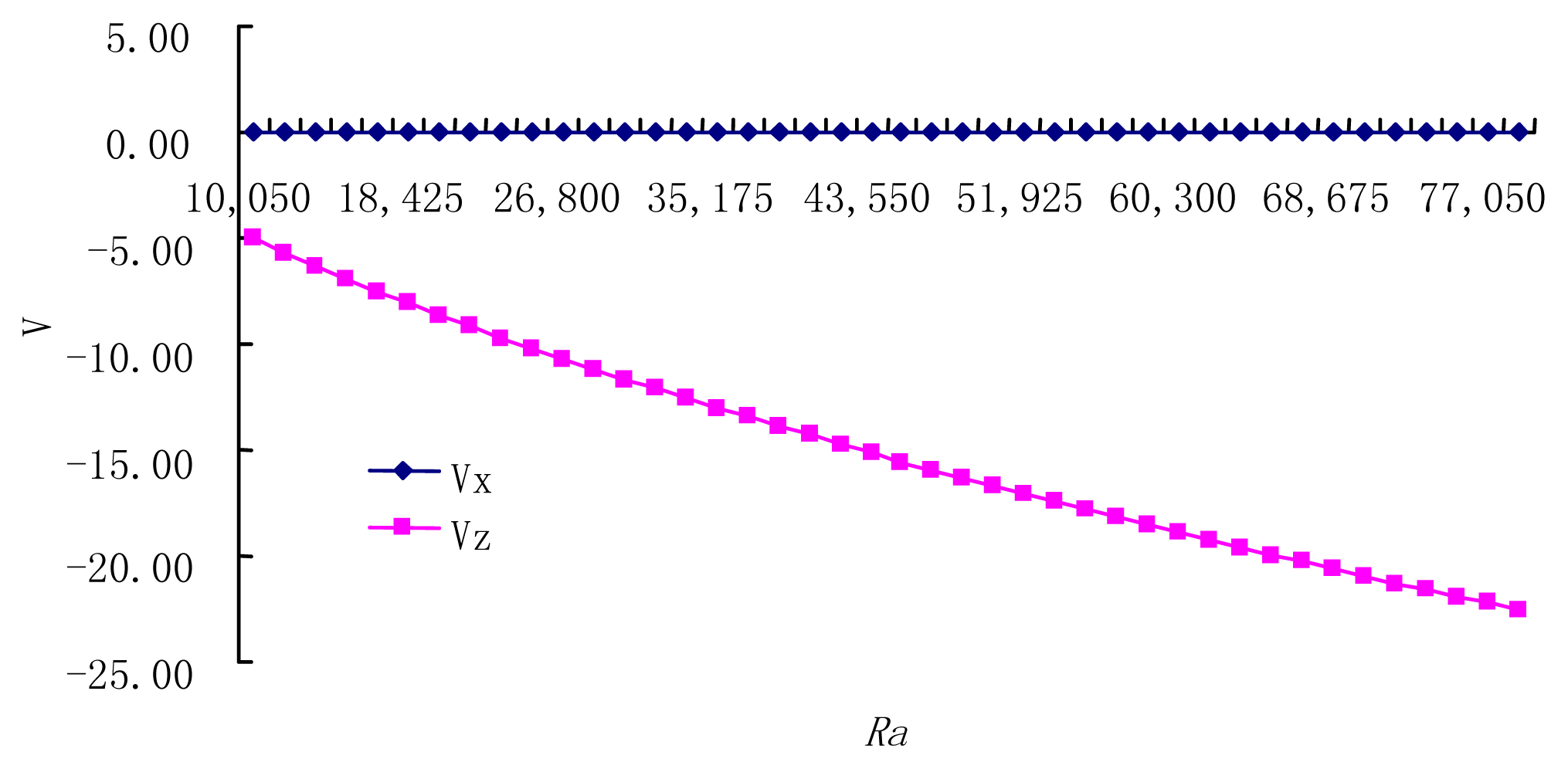
In a different simulation, the patterns of Bénard cells with two vortexes had a very small difference in the same model; while a different amount of energy is saved in steady Bénard flows with a different Ra. Figure 6 and Figure 7 show the steady temperature and speed change with Ra. In the figures, it is easy to see that the steady temperature and speed increase with an increase in the dimensionless parameter Ra. Additionally, the value of the dimensionless speed is larger than the dimensionless temperature. For the relationship between speed/temperature and energy, it is easy to know that the Bénard system turned into a more deluxe energy stage with an increase in the dimensionless parameter Ra. However, it is clear that for the Bénard flow in simulations with different dimensionless parameter Ra numbers, the external driving force is quite different: a Bénard flow with different dimensionless parameter Ra numbers must have the same rate of energy dissipation.
5.2. The Characteristics of Entropy Production in a Bénard Cell
5.2.1. Entropy Productions in Steady Bénard Flows with a Different Ra
Bénard convection develops at a steady rate when Ra numbers are different. The Bénard cell pattern difference is very small, similar to the flow pattern shown in Figure 5a. The variation rule of entropy productions, such as Sp and Sg, which were calculated by two different methods, varied with the dimensionless parameter Ra, shown in Figure 8. In Figure 8, it is clear that the entropy productions, Sp and Sg, are basically the same. Moreover, the entropy production increases with an increase in the dimensionless parameter Ra, in steady flow. This situation occurs due to the fact that when other parameters do not change, only the value of the dimensionless parameter Ra increases. As a result, the difference in temperature between the upper and lower level of the Bénard fluid’s surface grows larger and larger. The more energy flowing in to the system from outside, the system will achieve a higher energy state. According to the theory of entropy equilibrium, the system must then dissipate more energy outward in order to reach a steady state.
Two conclusions were drawn using the two methods of calculation, which were explained in Section 3: (1) The entropy production Sp, based on the theory of thermodynamics, is determined by the flow state and the universal entropy equilibrium equation. It can be regarded as the “true value” of the system’s entropy production, because it is suitable for any flow state. (2) The entropy production Sg based on the linear theory of non-equilibrium thermodynamics, is only suitable for a system in a state of near thermodynamic equilibrium. This is based on the “hypothesis of local equilibrium”, which was used in the process of derivation, considered as the “reference value” in this study. The level that the system deviates from the near-equilibrium thermodynamic zone can be calculated by comparing the actual value and the reference value. In Figure 8, the two curves that stand for entropy productions Sp and Sg are intertwined with each other and are difficult to discern. The chart shows that all of the states in this study were, in fact, in the near-equilibrium thermodynamic zone. Therefore, linear thermodynamic theory was a suitable method for exploring the Bénard convection phenomenon.
Figure 9 shows the difference between Sp and Sg (abbreviated Sp-Sg) varied with the dimensionless parameter Ra. Compare Figure 8 with the result in Figure 9, it is found that Sp-Sg is much smaller than entropy production in a fixed Ra, but it still has its own rule. In Figure 9, it is clear that the oscillation amplitude of Sp-Sg increases with an increase in the dimensionless parameter Ra. In other words, Sp-Sg gets a rude shock in larger Ra. According to the conclusions mentioned above, the system will get into a more complex deluxe energy stage with a larger Ra, and it is more and more difficult to reach a steady state. That is to say, Sp-Sg is in connection with the state of the system. When the system gets into a deluxe energy stage, the chance of getting a bigger value of Sp-Sg is more than for the system in the low energy stage.
5.2.2. The Driving Force of the Bénard System
The difference between Sp and Sg (Sp – Sg) is in connection with the state of the system, and it is the driving force for driving the system to a steady state. This phenomenon is reflected in the process of an unsteady Bénard system with any Ra development to a steady state. It was found in numerical simulations that all of the development of Bénard flow with a different Ra in this study has the nearly same process, and the results are the same as each other. For this reason, the dynamic process of a Bénard system with Ra = 16,750 was choose to study the phenomenon. It is worth noting that the calculation method of Sp has a little difference for the reason of the state of the system. In the dynamic process, the change in entropy is not equal to zero. It can be calculated by Equation (12).
In Equation (12), ΔS is the entropy change and C is the specific heat. In order to ensure the accuracy of the calculation, the specific heat C is gotten from Equation (13).
Figure 10 shows the two entropy productions, Sp and Sg, changing with time in the development process of the flow starts from the rest. In the unsteady system, the change of Sp with time is great, while the change of Sg with time is smaller. That is because the linear theory of non-equilibrium thermodynamics was used in the calculation of Sg. As can be seen from Figure 10, Sp – Sg has a greater value when the flow in a more complex state. When the system is in an unsteady state, Sp – Sg has a great difference. However, when the system reaches a steady state, Sp and Sg are basically the same. This means that there is some law in the difference between Sp and Sg and the states of the Bénard flows. When the system transitions from a complex, unsteady state to a simple, steady state, the difference between Sp and Sg gets smaller, and the phenomenon shows that Sp – Sg is the driving force to driving the system to a steady state.
5.3. The Character of the Spatial Distribution of Local Entropy Production
The spatial distribution of the local entropy production of Bénard cells with two steady vortexes has attracted researchers. A number of simulations have been done on this topic. In addition, simulations show that the spatial distribution of the local entropy production of Bénard cells with two steady vortexes is nearly the same. For this reason, the Bénard cell with Ra equal to 20,100 was chosen to illustrate the spatial distribution of the local entropy production.
In the non-equilibrium thermodynamics process of this study, there was a significant finding during the analysis of the spatial distribution of the local entropy production. Not only was entropy produced at all times in the entire region, but the source of that energy came from any part of the system. For this reason, identical steady Bénard cells with two vortexes and different Ra were used to study the spatial distribution of the local entropy production.
Figure 11 shows the spatial distribution of the local entropy production of a steady Bénard cell in which the dimensionless parameter Ra equaled 20,100. As shown in Figure 11, the spatial distribution of the local entropy production was symmetrical. There are two large areas where the local entropy production is the smallest in each cavity. Note the position of the Bénard vortex in the Bénard cell. Otherwise, the area of the smallest local entropy production was around the area of larger local entropy production. At the top, bottom and right (or the left) of the areas of the smallest local entropy production, each has an area of larger local entropy production; but, in the middle of the whole zone, two areas of larger local entropy production appeared. The local entropy production, though, was relatively small in the other position of the side wall. Therefore, the production centered on the local entropy production of smaller areas bordering the local entropy production of larger areas.
Using the second law of thermodynamics, we know that the areas of larger local entropy production occur where the macro movement is complex, as seen by comparing Figure 5a and Figure 11. Bénard cells form because the varied sizes of local entropy production areas form a stable combination. When the position of the local entropy production is ideal, Bénard cell vortexes form easily.
6. Conclusions
A large number of steady Bénard convection flows were obtained by changing the aspect ratio L/H of the Rayleigh–Bénard convection model, or the fluid’s dimensionless parameter Ra, in numerical simulations. This study found that in Bénard convection experiments, the dimensionless parameter Ra is crucial to the formation of a steady Bénard convection flow. The model’s aspect ratio L/H plays a major role in the pattern of the Bénard cell, as well. A series of steady Bénard flows with an L/H aspect ratio of two were used in this study to achieve the research objectives.
As far as this study’s more important conclusions, firstly, the Sp based on classical thermodynamics and the Sg based on the linear non-equilibrium thermodynamics provided the same results after calculation. Secondly, by comparing the two system’s entropy productions, it was found that the system of two entropy productions increases with the increase of the dimensionless parameter Ra in a Bénard flow. Thirdly, it was found that the difference between the two entropy productions (Sp – Sg) is the driving force for driving the system to a steady state. At last, the distribution of the Bénard cell’s local entropy production was found. The vortexes of Bénard cells are located in the minimum local entropy production bordering larger local entropy production.
This study could enrich people’s understanding of the Bénard convection phenomenon, provide additional information relevant to the study of far from equilibrium thermodynamics and may prove practically applicable in the field of engineering.
Acknowledgments
This work was supported by the Natural Science Foundation of China (Grant No. 50876092)
Author Contributions
Chenxia Jia established the model and performed the analytical calculations and the numerical simulations. Chengjun Jing proposed an approach to solve the problem. Jian Liu also did the numerical simulations on the entropy production in the non-steady state. All authors have read and approved the final published manuscript.
Conflicts of Interest
The authors declare no conflict of interest.
References
- Behringer, R.P. Rayleigh–Bénard convection and turbulence in liquid helium. Rev. Mod. Phys 1985, 57, 657–687. [Google Scholar]
- Townsend, A.A. Temperature fluctuations over a surface. J. Fluid Mech 1959, 5, 209–241. [Google Scholar]
- Rapaport, D.C. Time dependent patterns in atomistic ally simulated convection. Phys. Rev. A 1991, 43, 7046–7048. [Google Scholar]
- Sone, S.; Aokik, K.; Sugimoto, H.; Motohasi, H. The Benard problem of rarefied gas dynamics. In Rarefied Gas Dynamics; Volume 19, Oxford University Press: New York, NY, USA, 1995; pp. 154–196. [Google Scholar]
- Paul, S.; Wahi, P.; Verma, M.K. Bifurcations and chaos in large-Prandtl number Rayleigh–Bénard convection. Int. J. Non-Linear Mech 2011, 46, 772–781. [Google Scholar]
- Garcia, A.L.; Baras, F.; Mansour, M.M. Comment on “simulation of a two dimensional Rayleigh Benard system using the direct simulation Monte Carlo Method”. Phys. Rev. E 1995, 51. [Google Scholar] [CrossRef]
- Puhl, A.; Mansour, M.M.; Mareschal, M. Quantitative comparison of molecular dynamics with hydrodynamics in Rayleigh Benard convection. Phys. Rev. A 1989, 40, 1999–2012. [Google Scholar]
- Assenheimer, M.; Steinberg, V. Transition between spiraland target states in Rayleigh–Bénard convection. Nature 1994, 367, 345–347. [Google Scholar]
- Ning, L.Z. Rayleigh–Bénard convection in a binary fluid mixture with and without lateral flow; Northwest A & F University Press: Xi’an, China, 2006; pp. 1–11. (In Chinese) [Google Scholar]
- Goux, W.J.; Verkruyse, L.A.; Saltert, J.S. The impact of Rayleigh–Bénard convection on NMR pulsed-field-gradient diffusion measurements. J. Magn. Reson (1969) 1990, 88, 609–614. [Google Scholar]
- Wang, J.J.; Ma, X.Q. A study on the behavior of LNG after stratification in main stream region of storage tank. J. Hydrodyn 2007, 22, 31–35. [Google Scholar]
- Chen, Y.S. Non-linear vibration theory; Higher Education Press: Beijing, China, 2002. (In Chinese) [Google Scholar]
- Lai, Y.M.; Zhang, M.Y.; Yu, W.B. Experimental study on the cooling effect and mechanism of closed ripped-rock embankment. J. Glaciol. Geocryl 2004, 26, 576–581. (In Chinese) [Google Scholar]
- Barry, P.; Dan, M.K. Mantle convection and the thermal structure of the plates. J. Geophys. Res. Solid Earth 1978, 83, 4485–4496. [Google Scholar]
- Yeates, P.S.; Imberger, J. Pseudo two-dimensional simulations of internal and boundary fluxes in stratified lakes and reservoirs. Int. J. River Basin Manag 2003, 1, 297–319. [Google Scholar]
- Henderson-Sellers, B.; Davies, A.M. Thermal stratification modeling for oceans and lakes. Annu. Rev. Heat Transf 1989, 2, 86–156. [Google Scholar]
- Imberger, J.; Hamblin, P.F. Dynamics of lakes, reservoirs, and cooling ponds. Annu. Rev. Fluid Mech 1982, 14, 153–187. [Google Scholar]
- Niven, R.K. Simultaneous extrema in the entropy production for steady-state fluid flow in parallel pipes. J. Non-Equil. Thermody 2010, 35, 347–378. [Google Scholar]
- Kawazura, Y.; Yoshida, Z. Comparison of entropy production rates in two different types of self-organized flows: Bénard convection and zonal flow. Phys. Plasmas 2012, 19. [Google Scholar] [CrossRef]
- Jia, C.X.; Huo, H.E.; Jing, C.J.; Qin, P. An application of Lyapounov theory to of the stability analysis of thermal convection system. J. Therm. Sci. Tech 2010, 9, 1–5. [Google Scholar]
Figure 1.
The Rayleigh–Bénard model.

Figure 2.
Staggered mesh format.
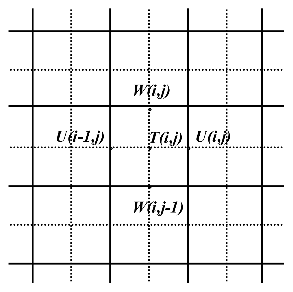
Figure 3.
The computational mesh actually in use.
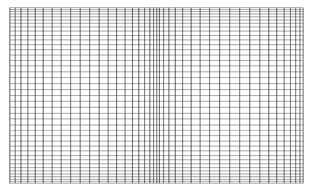
Figure 4.
Comparison of entropy production with different time steps.

Figure 5.
Bénard cells obtained in the simulation. (a) Bénard cells with two vortexes. (b) Bénard cells with four vortexes. (c) Bénard cells with six vortexes.
Figure 5.
Bénard cells obtained in the simulation. (a) Bénard cells with two vortexes. (b) Bénard cells with four vortexes. (c) Bénard cells with six vortexes.

Figure 6.
The steady temperature change with Ra.
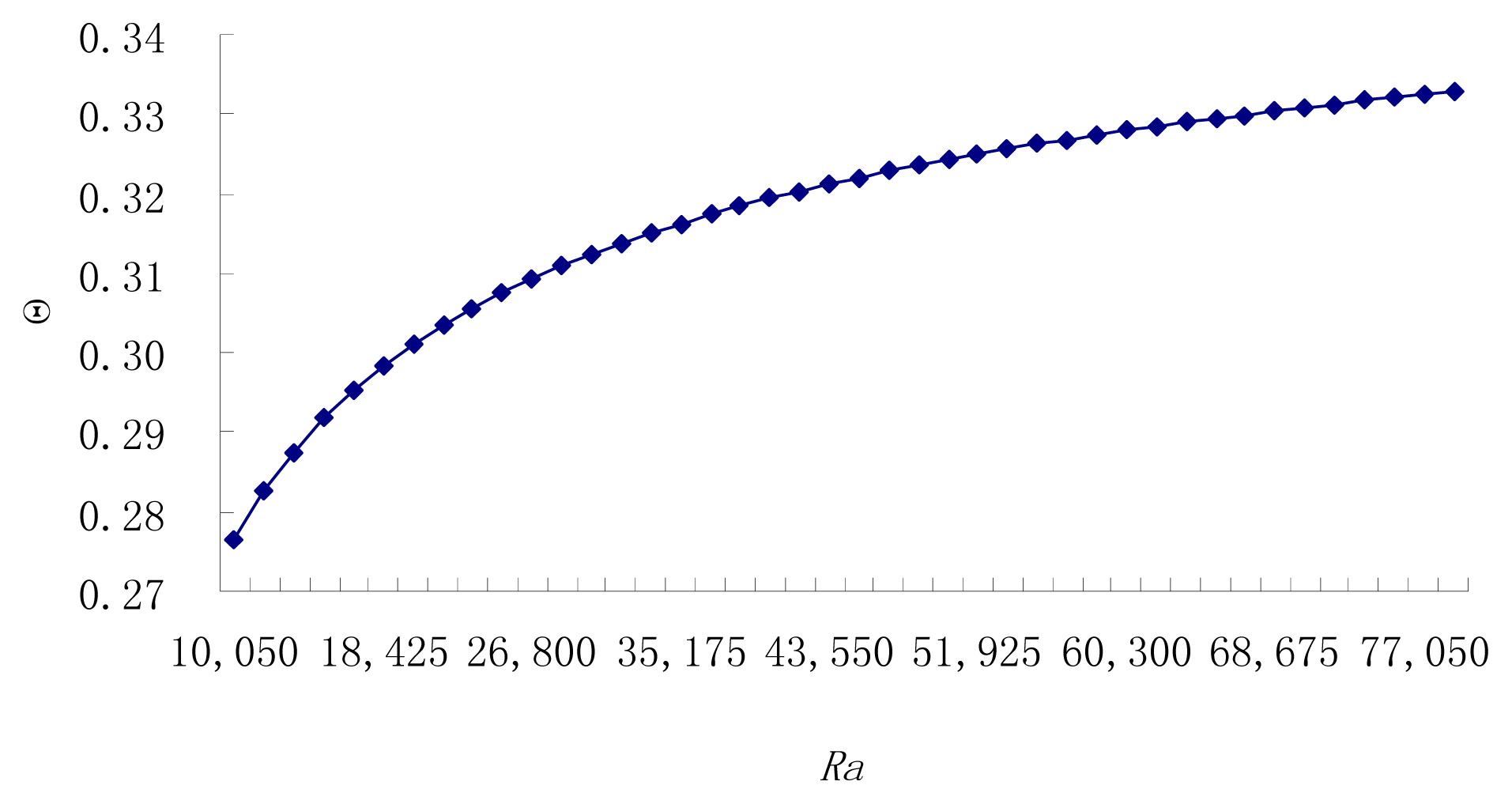
Figure 7.
The steady speed change with Ra.

Figure 8.
Entropy productions Sp or Sg change with Ra.
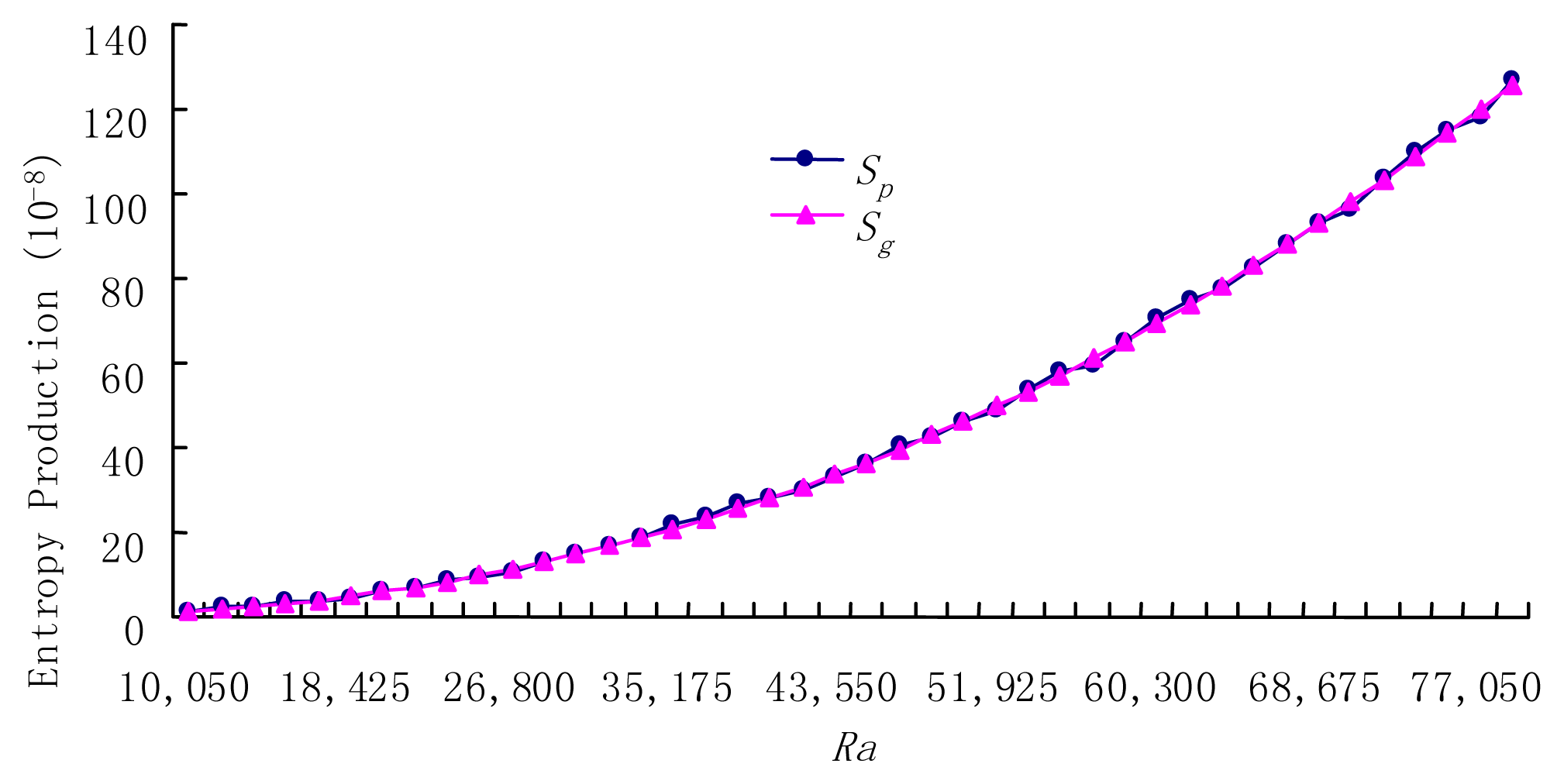
Figure 9.
The difference between the two entropy productions change with Ra.
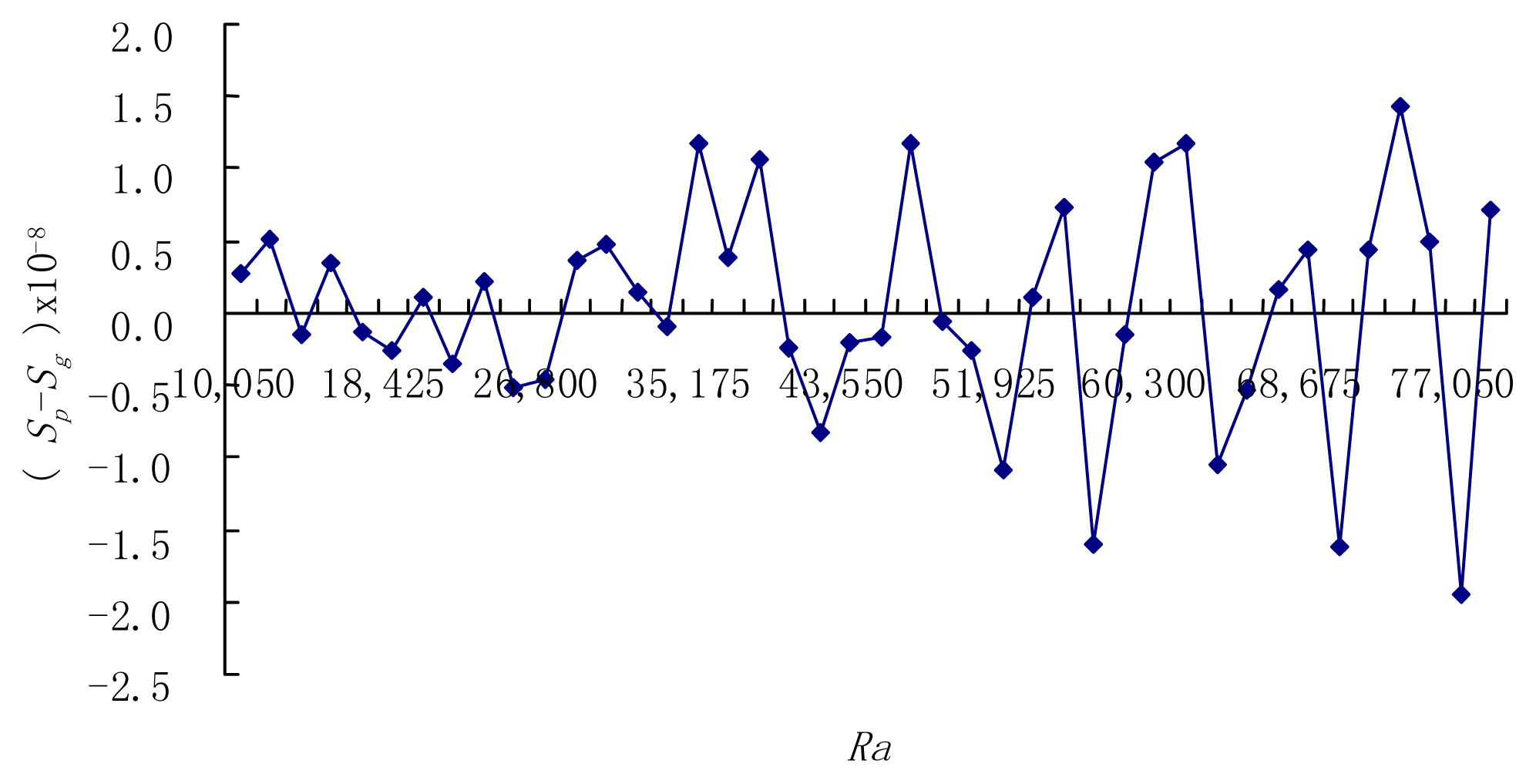
Figure 10.
The two entropy productions change with time (Ra = 20, 100).
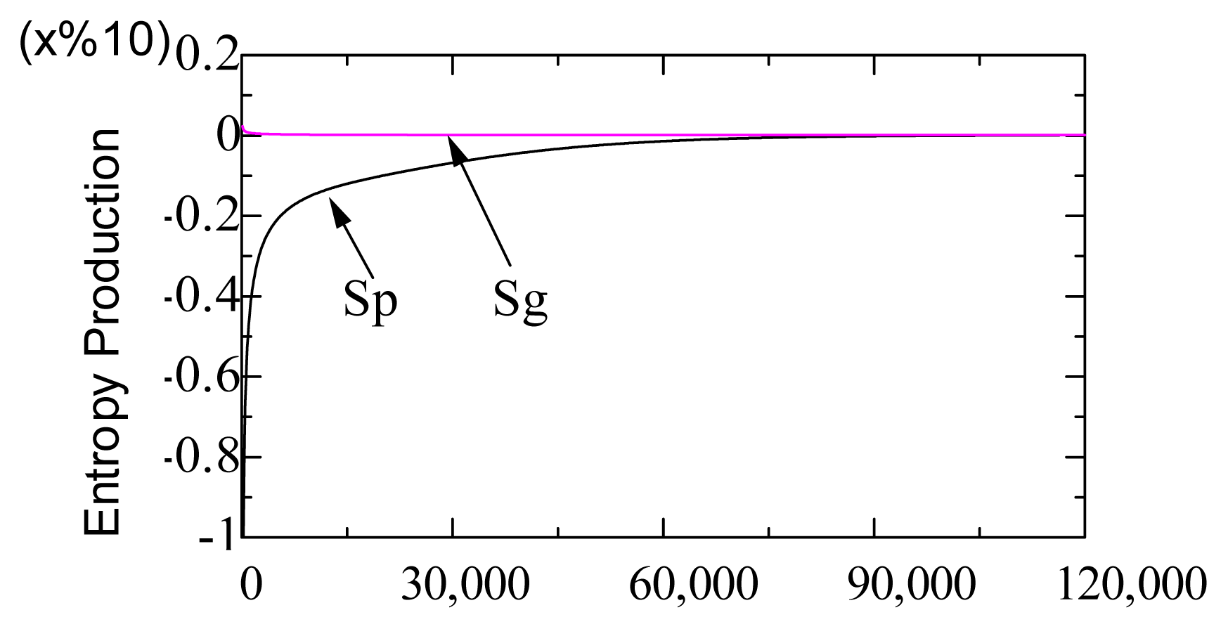
Figure 11.
The local entropy produce distribution in stable simulation of Ra = 20, 100.

© 2014 by the authors; licensee MDPI, Basel, Switzerland This article is an open access article distributed under the terms and conditions of the Creative Commons Attribution license (http://creativecommons.org/licenses/by/3.0/).
Share and Cite
MDPI and ACS Style
Jia, C.; Jing, C.; Liu, J. The Character of Entropy Production in Rayleigh–Bénard Convection. Entropy 2014, 16, 4960-4973. https://doi.org/10.3390/e16094960
AMA Style
Jia C, Jing C, Liu J. The Character of Entropy Production in Rayleigh–Bénard Convection. Entropy. 2014; 16(9):4960-4973. https://doi.org/10.3390/e16094960
Chicago/Turabian StyleJia, Chenxia, Chengjun Jing, and Jian Liu. 2014. "The Character of Entropy Production in Rayleigh–Bénard Convection" Entropy 16, no. 9: 4960-4973. https://doi.org/10.3390/e16094960