Using Geometry to Select One Dimensional Exponential Families That Are Monotone Likelihood Ratio in the Sample Space, Are Weakly Unimodal and Can Be Parametrized by a Measure of Central Tendency

Abstract

One dimensional exponential families on finite sample spaces are studied using the geometry of the simplex ${\Delta }_{n-1}^{°}$ and that of a transformation V_n−1 of its interior. This transformation is the natural parameter space associated with the family of multinomial distributions. The space V_n−1 is partitioned into cones that are used to find one dimensional families with desirable properties for modeling and inference. These properties include the availability of uniformly most powerful tests and estimators that exhibit optimal properties in terms of variability and unbiasedness.

1. Introduction

The motivation for the constructions in this paper begins with a sample from a one dimensional space that is discrete. We allow for a continuous sample space but assume that this has been suitably discretized into n bins. The simplest underlying structure for the probability assigned to these bins is given by the multinomial distribution. The collection of all multinomial distributions can be identified with the n − 1 simplex Δ_n−1. We use the geometry of the simplex along with a transformation of its interior ${\Delta }_{n-1}^{°}$ to search for one dimensional subspaces that have good properties for modeling and for inference. In particular, we want families that can be parameterized by the mean, have only unimodal distributions, have desirable test characteristics (such as providing uniformly most powerful unbiased tests) and estimation properties (such as unbiasedness and small variability).

The boundary of the (n − 1) dimensional simplex Δ_n−1 can be written as the union of simplexes of dimension (n − 2). This process can be repeated on the simplexes of lower dimension until the boundary consists of the vertices of the original simplex. This construction has statistical relevance to the possible supports for the probability distributions considered on the n bins. We obtain a dual decomposition for a transformation V_n−1 (defined in Equation (5) in Section 5) of ${\Delta }_{n-1}^{°}$; it is dual in that the result can be obtained by replacing simplexes with cones. The statistical relevance of the conical decomposition is to the possible modes for all the distributions on the n bins. Since V_n−1 is the natural parameter space for the distributions in ${\Delta }_{n-1}^{°}$, one dimensional exponential families are lines in V_n−1 and these can be related to the cones that partition V_n−1. One result is that the limiting distribution for any one dimensional exponential family in ${\Delta }_{n-1}^{°}$ is the uniform distribution whose support is determined by the cone that contains the limiting values of the line corresponding to the exponential family.

While one parameter exponential families can be defined quite generally by choosing a sufficient statistic, it can be useful to start with the sufficient statistics from well-known families such as the binomial, Poisson, negative binomial, normal, inverse Gaussian, and Gamma distribution. These exponential families have good modeling and inferential properties that we try to maintain by limiting the extent to which the sufficient statistic is modified. These restrictions lead to considering vectors in V_n−1 that lie in a cone. Examples of how to construct these cones are given.

2. Motivating Examples

One dimensional exponential families such as the binomial or Poisson are the workhorse of parametric inference because of their excellent statistical properties. However, being one dimensional means they do not always fit data very well so an extension to a two (or higher) dimensional exponential family can be pursued in order to preserve the nice inferential structure. An issue with such extension is that, for each extra natural parameter added, we need to choose a new sufficient statistic and this choice can substantially change the shape of the corresponding density functions. For example densities can pass from being unimodal to have multiple modes for some parameter values. To see this, consider the following examples.

Example 1. Altham [1] considered the so-called multiplicative generalization of the binomial distribution with corresponding density

$$f(x;p,\varphi )=\left(\begin{array}{c}n\\ x\end{array}\right)p^x{(1-p)}^{n-x}{\varphi }^{x(x-n)}/C(p,\varphi )$$

(1)

where C is the normalizing constant and where clearly the binomial is recovered when ϕ = 1.

By reparametrizing using θ₁ = log(p/(1 − p)) and θ₂ = log(ϕ) this density can be expressed in exponential form as

$$f(x;{\theta }_1,{\theta }_2)=h(x)\text{exp}({\theta }_{1}x+{\theta }_{2}T(x)-K({\theta }_1,{\theta }_2))$$

(2)

where T (x) = x(x − n) is the added sufficient statistic and$h(x)=\left(\begin{array}{c}n\\ x\end{array}\right)$ where dependence on n has been ignored. Note that the same family is obtained if T (x) = x² is added as a sufficient statistic instead of x(x − n).

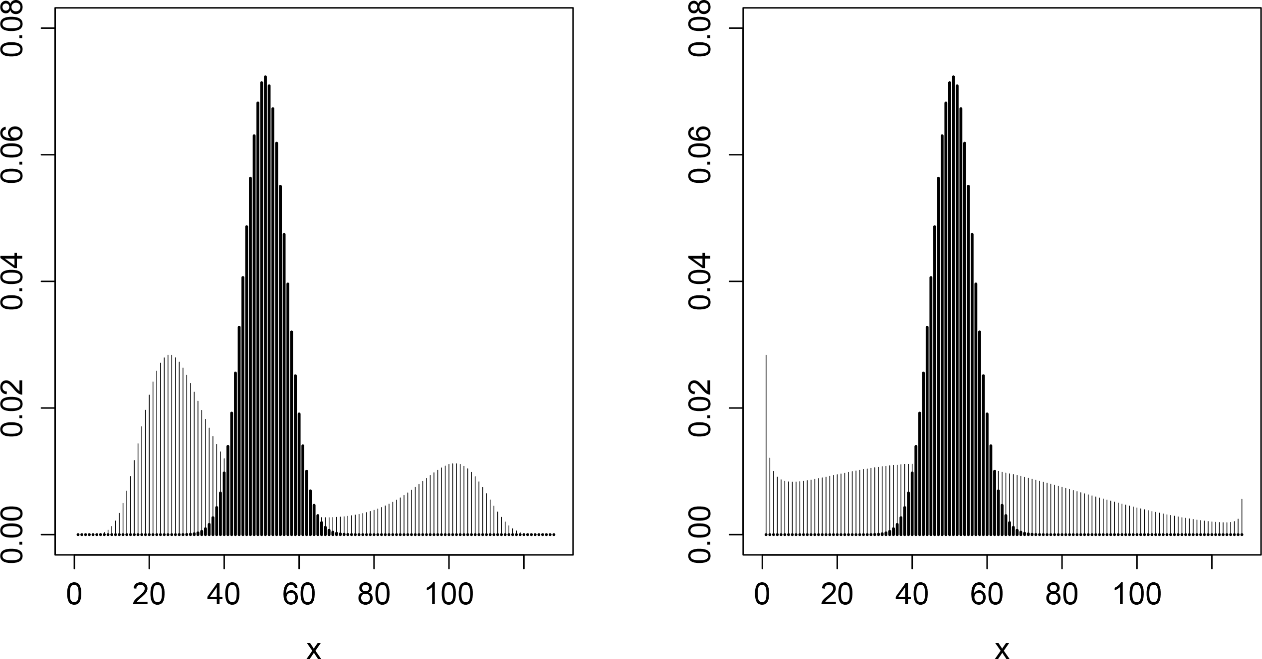
If n = 127 and (θ₁, θ₂) = (−0.0122, 0.018) then density (2) is bimodal as shown in the left panel of Figure 1. The mean μ of this distribution is 50. Also plotted is the corresponding binomial density with the same mean or equivalently with θ₁ = log(50/(127 − 50)) = −0.4318 and θ₂ = 0.

As explained by Lovison [2], this distribution has the feature of being under- or over-dispersed with respect to the binomial depending on θ₂ being negative or positive, respectively. Furthermore, using the mixed parametrization (μ, θ₂) (see [3] for details) it is easy to see that this distribution can be parametrized so that one parameter controls dispersion independently of the mean. In fact, for a fixed mean μ, as θ₂ → −∞ f(x; θ₁, θ₂) tends to a two point distribution (with support points at the extremes x = 0 and x = n) or to a degenerate distribution on x = μ when θ₂ → ∞.

Example 2. Double exponential families [4] are two parameter exponential families that extend standard unidimensional exponential families such as the binomial and the Poisson. Similar to the multiplicative binomial in Example 1, the extra parameter involved in double exponential families controls the variance independently of the mean. The density for the so-called double binomial family can be written in the form (2) with

$$T(x)=x\text{log}\left(\frac{x}{n}\right)+(n-x)\text{log}\left(1-\frac{x}{n}\right)$$

$h(x)=\left(\begin{array}{c}n\\ x\end{array}\right)$ and with the particular restriction that θ₂ < 1 (see [4] for details). The range θ₂ < 0 generates underdispersion and θ₂ ∈ [0, 1) generates overdispersion with respect to the binomial. As shown on the right panel of Figure 1, the double binomial density can also be multimodal where the double binomial density shown has the same mean and variance as the multiplicative binomial shown in the left panel.

These examples show that while extending exponential families can lead to useful modeling properties such as overdispersion, the extension can also result in distributions that are not suitable for modeling. We are interested in the relationship between geometric properties of one dimensional families and the modeling properties of their distributions.

3. Sample Space and Distribution-valued Random Variables

We consider first the general case where the sample space for a single observation X₁ consists of n bins

$$S_n=\{B_1,B_2,\dots ,B_{n-1},B_n\}.$$

We consider the space of all probability distributions $𝒫$ on this sample space S_n. Each probability distribution in $𝒫$ is defined by the n-tuple p whose i^th component is

$$p^i=\text{Pr}(B_i)$$

so that $𝒫$ can be identified with the n − 1 simplex

$${\Delta }_{n-1}=\{p\in {ℝ}^n:p^i\ge 0\hspace{0.17em}\hspace{0.17em}\forall i,\hspace{0.17em}\hspace{0.17em}{1}^{\prime }p=1\}$$

where 1 in 1′p is the vector 1 ∈ ℝⁿ each of whose components is 1. We will slightly abuse the notation by using p to name a point in Δ_n−1, and hence in ℝⁿ, as well as the corresponding distribution in $𝒫$.

The sample space for a random sample of size N from a distribution p₀ ∈ Δ_n−1 is

$${𝒳}_n^N=\{x:x\hspace{0.17em}\text{is}\hspace{0.17em}\text{an}\hspace{0.17em}n\hspace{0.17em}\text{vector}\hspace{0.17em}\text{of}\hspace{0.17em}\text{nonnegative}\hspace{0.17em}\text{integers}\hspace{0.17em}\text{that}\hspace{0.17em}\text{sum}\hspace{0.17em}\text{to}\hspace{0.17em}N\}$$

There is simple relationship between ${𝒳}_n^N$ and the simplex that we obtain by dividing each component of x by N. Although the sample space ${𝒳}_n^N$ can be viewed as formed by compositional data, we will follow a different approach to handle this kind of data compared with the classical approach described by Aitchison [5] because the data we consider have additional structure.

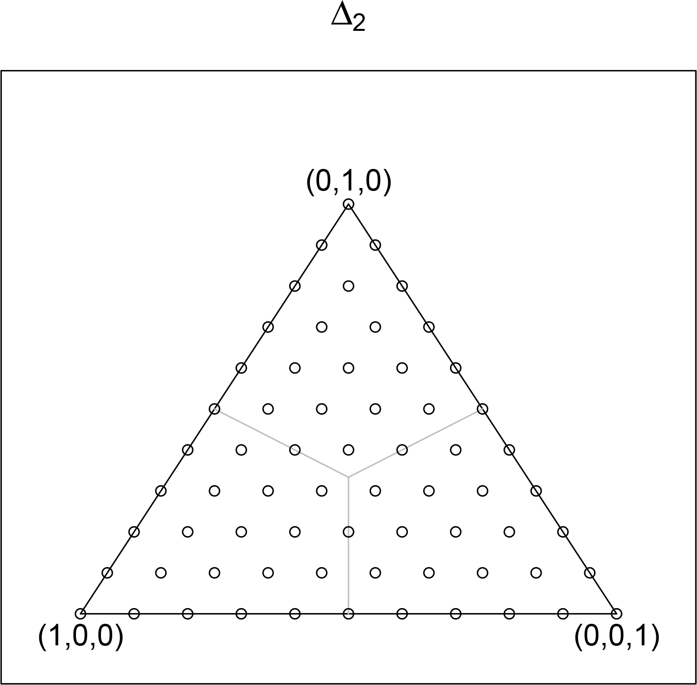
In Figure 2 the sample space for the sample of size N = 10 is displayed using open circles. The vertices correspond to the case where all 10 values fall in a single bin. The other points correspond to the less extreme cases. Let p₀ be any point in Δ_n−1. By mapping the multinomial random variable of counts X to Δ_n−1, we obtain the random distribution P̂ = X/N whose values are multinomial distributions each having number of cases N and probability vector X/N. Identifying ${𝒳}_n^N$ -valued random variables with distribution-valued random variables provides a natural means for comparing data with probability models using the Kullback–Leibler (KL) divergence.

We can compare distributions in Δ_n−1 using the KL divergence D : $𝒫$ × $𝒫$ ↦ ℝ

$$D(p_1,p_2)=\sum p_1\text{log}(p_1/p_2)=H(p_1,p_2)-H(p_1)$$

where H(p₁, p₂) = − ∑p₁ log(p₂) and H(p₁) = H(p₁, p₁) is the entropy of p₁. Note that the arguments to D and H are distributions while the logarithm and ratios are defined on points in ℝⁿ. Following Wu and Vos [6], the variance of the random distribution P̂ is defined to be

$${\text{Var}}_{p_0}(\widehat{P})=\underset{p\in {\Delta }_{n-1}}{\text{min}}{E}_{p_0}D(\widehat{P},p)$$

and its mean is defined to be

$${\text{E}}_{p_0}(\widehat{P})=\text{arg}\underset{p\in {\Delta }_{n-1}}{\text{min}}{E}_{p_0}D(\widehat{P},p).$$

Note that the expectation on the right hand side of the equations above are for real-valued random variables while the expectation on the left hand side of the second equation is for a distribution-valued random variable.

It is not difficult to show that E_p0 P̂ = p₀ so that P̂ can be considered an unbiased estimator for p₀. Details are in [6], which also shows that the KL risk can be decomposed into bias-squared and variance terms:

$$E_{p_0}D(\widehat{P},q)=D(p_0,q)+{\text{Var}}_{p_0}(\widehat{P}).$$

The distributional variance is related to the entropy

$${\text{Var}}_{p_0}(\widehat{P})=E_{p_0}D(\widehat{P},p_0)=H(p_0)-E_{p_0}H(\widehat{P}).$$

Note that for N = 1, H(P̂) = 0 so that for a single observation the random distribution P̂ taking values on the vertices of Δ_n−1 has variance equal to the entropy of p₀.

For inference, p₀ is unknown but we specify a subspace M ⊂ Δ_n−1 that contains p₀, or at least has distributions that are not too different from p₀. Estimates can be obtained by choosing a parameterization for M, say θ, and then considering real-valued functions θ̂ and evaluating these in terms of bias and variance. Bias and variance are useful descriptions when θ describes a feature of the distribution that is of inherent interest. However, if θ is simply a parameterization, or if there are other features that are also of interest, then these quantities are less useful. For inference regarding the distribution p₀ we can use a distribution-valued estimator P̂_M where the subscript indicates that the estimator is defined to account for the fact that p₀ ∈ M.

We will not pursue the details of distribution-valued estimators here; we mention these only because all the subspaces we consider will be exponential families and in this case the maximum likelihood estimator has important properties in terms of distribution variance and distribution bias: when M is an exponential family, the maximum likelihood estimator is distribution unbiased, and it uniquely minimizes the distribution variance among the class of all distribution unbiased estimators. Furthermore, when p₀ ∉ M then the maximum likelihood estimator is the unique unbiased minimum distribution variance estimator of the distribution in M that is closest (in terms of KL) to p₀. Extensions of one dimensional exponential families that do not result in exponential families will not enjoy these properties of maximum likelihood estimation. Details of these results that hold for sample spaces more general than S_n are in [7].

4. Simplices Δ_s

One dimensional exponential families on S_n are curves in Δ_n−1 whose properties will depend on their location within various subspaces of Δ_n−1. An important collection of subspaces will be indexed by the subsets of S_n. For notational convenience we take B_i to the integer i. Using integers is suggestive of an ordering and a scale structure but at this point these are only being used to indicate distinct bins.

For each s ⊂ S_n,

$${\Delta }_s=\{p\in {ℝ}^n:p^i\ge 0\hspace{0.17em}\hspace{0.17em}\hspace{0.17em}\forall i\in s,\hspace{0.17em}\hspace{0.17em}{p}^i=0\hspace{0.17em}\hspace{0.17em}\hspace{0.17em}\forall i\in s^c,1^{\prime }p=1\}$$

where s^c = {i ∈ S_n : i ∉ s}. Note that Δ_Sn = Δ_n−1. The interior of Δ_s is

$${\Delta }_s^{°}=\{p\in {\Delta }_s:p^i>0\hspace{0.17em}\hspace{0.17em}\forall i\in s\}.$$

As probability distributions in $𝒫$, ${\Delta }_s^{°}$ corresponds to the set of all distributions having support s. There is a simple and obvious relationship between the dimension of Δ_s, |Δ_s|, and the cardinality of s, |s|, which holds for all nonempty s ⊂ S_n

$$\left|{\Delta }_s\right|+1=\left|s\right|.$$

The boundary of Δ_s is defined as

$$\partial {\Delta }_s=\{p\in {\Delta }_s:p\notin {\Delta }_s^{°}\}$$

so that

$${\Delta }_s={\Delta }_s^{°}\uplus \partial {\Delta }_s$$

where ⊎ indicates the sets in the union are disjoint. The boundary ∂Δ_s can be written as the union of all simplices of dimension one less than that Δ_s

$$\partial {\Delta }_s=\underset{s^{\prime }:s^{\prime }\subset s,\hspace{0.17em}\hspace{0.17em}\hspace{0.17em}\left|s^{\prime }\right|=\left|s\right|-1}{\cup }{\Delta }_{s^{\prime }}$$

(3)

This boundary property for Δ_s holds because the simplex $𝒮$_n consists of all possible subsets. Each nonempty s ∈ $𝒮$_n specifies one of the possible supports for distribution P ∈ $𝒫$_n

$${\Delta }_s=\underset{s^{\prime }:s^{\prime }\subset s}{\uplus }{\Delta }_{s^{\prime }}^{°}$$

(4)

where we set Δ_∅ = ∅.

5. Cones Λ_s

The set of all nonempty subsets of the sample space provides a partition of Δ_n−1 based on the support of the distributions in $𝒫$. The elements in the partition are simplices whose dimension is one less than the cardinality of the indexing set. In most cases we will consider models having support S_n, that is, models corresponding to ${\Delta }_{n-1}^{°}$. If we use subsets s to define the mode rather than support, we obtain a partition of $𝒫$°, the distributions in $𝒫$ having support S_n. This partition can be expressed using convex cones in an n − 1 dimensional plane V_n−1. The dimension of the cones are n minus the cardinality of the indexing set and the relationship between interiors of cones and their boundaries is analogous to that for simplices expressed in Equations (3) and (4).

Let

$$V_{n-1}=\{v\in {ℝ}^n:1^{\prime }v=0\}$$

(5)

be the subspace of ℝⁿ of dimension n−1 of all vectors that sum to zero. For each nonempty s ∈ S_n define

$${\Lambda }_s=\left\{v\in {\text{V}}_{n-1}:v^i\ge v^i\hspace{0.17em}\hspace{0.17em}\hspace{0.17em}\forall i\in s,\hspace{0.17em}\hspace{0.17em}\hspace{0.17em}\forall j\in S_n\right\}.$$

It is easily checked that Λ_s is a convex cone

$$v_1,v_2\in {\Lambda }_s\Rightarrow a_1{v}_1+a_2{v}_2\in {\Lambda }_s\hspace{0.17em}\hspace{0.17em}\hspace{0.17em}\hspace{0.17em}\hspace{0.17em}\hspace{0.17em}\forall a_1,a_2\in \left[0,\infty \right).$$

The dimension of Λ_s is |Λ_s| = n −|s| since each point in j ∈ s^c provides a basis vector b_j whose i^th component is 1 if i ∈ s or i = j and is zero otherwise and |s^c| = n −|s|. The interior of Λ_s is

$${\Lambda }_s^{°}=\left\{v\in {\Lambda }_s:v^i>v^j\hspace{0.17em}\hspace{0.17em}\hspace{0.17em}\forall i\in s,\hspace{0.17em}\hspace{0.17em}\hspace{0.17em}\forall j\in s^c\right\},$$

the boundary is

$$\partial {\Lambda }_s=\left\{v\in {\Lambda }_s:v\notin {\Lambda }_s^{°}\right\},$$

so that

$${\Lambda }_s={\Lambda }_s^{°}\uplus \partial {\Lambda }_s$$

by definition. Note ${\Lambda }_{S_n}={\Lambda }_{S_n}^{°}=0\in {\text{V}}_{n-1}\subset {ℝ}^n$ where the first equality holds because the conditions in the definition of ${\Lambda }_s^{°}$ hold vacuously since $i\in S_n^c=\varnothing$ adds no restriction. Likewise, we can extend the definition of Λ_s to include s = ∅ and since i ∈ ∅ adds no restriction

$${\Lambda }_{\varnothing }={\Lambda }_{\varnothing }^{°}={\text{V}}_{n-1}.$$

Note that Λ_∅ depends on the cardinality of the set S_n. Since we are considering n fixed, we will not show this dependence in the notation.

Corresponding to Equation (3) we have for all nonempty s that the boundary of the cone Λ_s is the union of all cones having dimension one less than the dimension of Λ_s

$$\partial {\Lambda }_s=\underset{s^{\prime }:s^{\prime }\subset s,\hspace{0.17em}\hspace{0.17em}\hspace{0.17em}\left|s^{\prime }\right|=\left|s\right|+1}{\cup }{\Lambda }_{s^{\prime }}$$

(6)

Corresponding to Equation (4) we have

$${\Lambda }_s=\underset{s^{\prime }:s\subset s^{\prime }}{\uplus }{\Lambda }_{s^{\prime }}^{°}$$

(7)

The relationship between the simplices Δ and cones Λ is more easily seen if we suppress the sets that index these objects. Let Δ and Δ_* be any two simplices and let Λ and Λ_* be any two convex cones. We only consider cones and simplices that correspond to a nonempty subset of S_n. Then the Equations (6) and (7) for the convex cones are obtained by simply replacing Δ in Equations (3) and (4) with Λ:

$$\partial \Delta =\underset{{\Delta }_{*}:\left|{\Delta }_{*}\right|=|\Delta |-1}{\cup }{\Delta }_{*},\hspace{0.17em}\hspace{0.17em}\hspace{0.17em}\hspace{0.17em}\hspace{0.17em}\partial \Lambda =\underset{{\Lambda }_{*}:\left|{\Lambda }_{*}\right|=|\Lambda |-1}{\cup }{\Lambda }_{*}$$

(8)

$$\Delta =\underset{{\Delta }_{*}\subset \Delta }{\uplus }{\Delta }_{*}^{°},\hspace{0.17em}\hspace{0.17em}\hspace{0.17em}\hspace{0.17em}\hspace{0.17em}\hspace{0.17em}\hspace{0.17em}\hspace{0.17em}\hspace{0.17em}\hspace{0.17em}\hspace{0.17em}\hspace{0.17em}\hspace{0.17em}\hspace{0.17em}\Lambda =\underset{{\Delta }_{*}\subset \Lambda }{\uplus }{\Lambda }_{*}^{°}$$

(9)

Equation (9) also holds for the empty set since Δ_∅ = ∅ and Λ_∅ = V_n−1.

6. V_n−1 and $𝒫$°

There is a natural bijection ϕ between V_n−1 and ${\Delta }_{n-1}^{°}$ defined by

$$\varphi (p)=\text{log}(p)-m(p)1$$

where log(p) is the vector with i^th component log(pⁱ) and m(p) is defined so that 1 ϕ(p) = 0. The inverse is

$$\phi (v)=k^{-1}(v)\text{exp}(v)$$

where exp(v) is the vector with i^th component exp(vⁱ) and k(v) is defined so that 1′ exp(v) = 1.

Each cone ${\Lambda }_s^{°}$ in the partition

$${\text{V}}_{n-1}=\uplus {\Lambda }_s^{°}$$

corresponds to one of the 2ⁿ − 1 possible modes for any distribution having support S_n since vⁱ > v^j if and only if φⁱ(v) > φ^j(v).

7. V_n−1 and Exponential Families in $𝒫$°

We define a line by a pair of vectors v₀, v₁ ∈ V_n−1 with v₁ ≠ 0

$$\ell =\ell (t)=\{v\in {\text{V}}_{n-1}:v=v_0+t{v}_1,\hspace{0.17em}\hspace{0.17em}\hspace{0.17em}t\in ℝ\}$$

Note that v₀ and v₁ are not unique. Applying the inverse transformation φ to points in ℓ gives probability densities

$$\phi (v_0+t{v}_1)=\frac{\text{exp}(v_0+t{v}_1)}{1^{\prime }\text{exp}(v_0+t{v}_1)}$$

(10)

which have the exponential family form with t playing the role of the natural parameter. Therefore, the space V_n−1 is easily recognized as the natural parameter space for the distributions ${\Delta }_{n-1}^{°}$ so that each line ℓ in V_n−1 corresponds to a one dimensional exponential family.

For each line ℓ(t) there is a value t_max such that {(t): t ≥ t_max} is contained in one of the cones ${\Lambda }_s^{°}$ where s is the subset of S_n with the property that $v_1^i\ge v_1^j$ for all i ∈ s for vectors $v_1\in {\Lambda }_x^{°}$. For each line ℓ(t) there is a value t_min such that {(t): t ≤ t_min} is contained in one of the cones ${\Lambda }_{s^{\prime }}^{°}$ where s′ is the subset of S_n with the property that $v_1^i\le v_1^j$ for all i ∈ s′ for vectors $v_1\in {\Lambda }_x^{°}$. The cones ${\Lambda }_s^{°}$ and ${\Lambda }_{s^{\prime }}^{°}$are disjoint and will be called the extremal cones for ℓ. There is at least one other cone ${\Lambda }_{s^{″}}^{°}$ such that $\ell \cap {\Lambda }_{s^{″}}^{°}\ne \varnothing$.

Any one dimensional exponential family ℓ(t) can be described by an ordered sequence of disjoint cones

$$({\Lambda }_{s_1}^{°},{\Lambda }_{s_2}^{°},\dots ,{\Lambda }_{s_k}^{°})$$

where k = k(ℓ) will depend on the family. These are simply the cones that are traversed by ℓ(t) between its extremal cones. We take ${\Lambda }_{s_k}^{°}$ to be the cone that contains ℓ(t) for all sufficiently large t. Equation (6) for cones means that

$$\partial {\Lambda }_{s_i}\subset {\Lambda }_{s_j}\hspace{0.17em}\hspace{0.17em}\text{for}\hspace{0.17em}\hspace{0.17em}\hspace{0.17em}j=i+1\hspace{0.17em}\hspace{0.17em}\text{or}\hspace{0.17em}\hspace{0.17em}\hspace{0.17em}j=i-1$$

The ordered sequence of cones provides an ordered sequence of unique subsets of S_n

$$(s_1,s_2,\dots ,s_k)$$

that we call the modal profile for ℓ as these are the modes realized by the exponential family ℓ(t) between its extremal cones that have modes s₁ and s_k.

Each point on a line ℓ(t) in V_n−1 corresponds to a distribution having support S_n. As t goes to −∞ (+∞) φ((t)) goes to a distribution having support s₁ (s_k). In fact, these are the uniform distribution on these supports. For every s ⊂ S_n other than ∅ and S_n, the uniform distribution on s is a limiting distribution for some one dimensional exponential family in $𝒫$°.

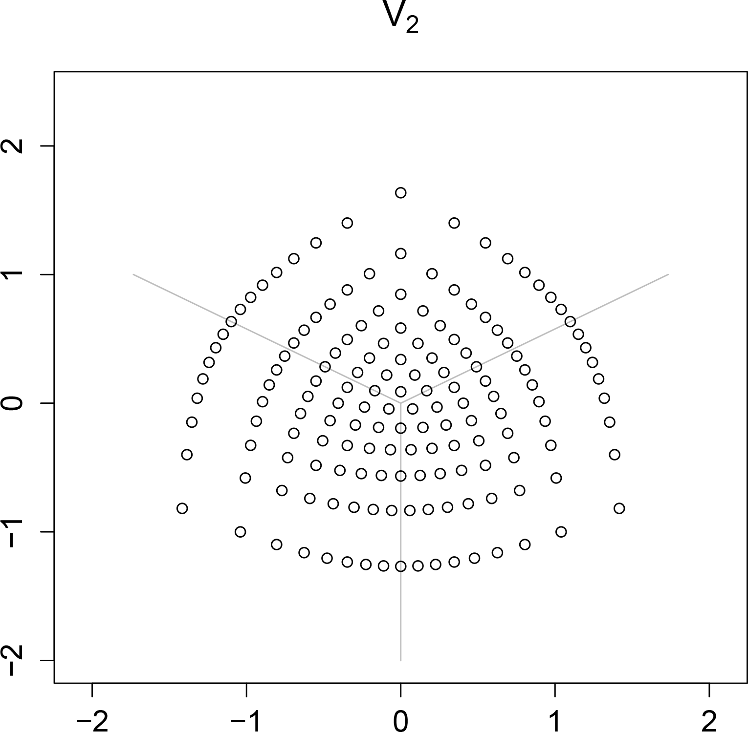
Figure 3 shows V_n−1 for the two dimensional simplex shown in Figure 2. The three rays are the one dimensional cones and the spaces between these cones are the two dimensional cones. The origin is the zero dimensional cone. The sample values on the boundary of Δ₂ are not in V₂. Note that the one dimensional cones are line segments in Δ₂.

8. Ordered Bins and the Monotone Likelihood Ratio Property

Let the bins be ordered and assign the first n integers to the bins to reflect this ordering. We seek to define exponential families that have a modal profile of the form

$$\left(\left\{1\right\},\{1,2\},\left\{2\right\},\{2,3\},\dots \{n-1,n\},\left\{n\right\}\right)$$

(11)

or a contiguous sub-collection of this profile. Extensions to three or more contiguous modes are clearly possible but not discussed here.

From the definition of modal profile, it follows that a family with modal profile (11) will have the property that the mode is a non-decreasing function of t. In addition to this property for the mode, we want the likelihood ratio for any two members of the family to provide the same ordering structure as that of the bins. A family that satisfies this condition is said to have the monotone likelihood ratio property with respect to x where x takes the values of the bin labels: 1, 2,...,n. Let p_θ1 and p_θ2 be two distributions in a one dimensional family parameterized by θ and let p_θ2/p_θ1 be the n-vector with components $p_{{\theta }_2}^j/p_{{\theta }_1}^j$ for 1 ≤ j ≤ n. This family has monotone likelihood ratio if for all θ₁ < θ₂ and j < j′

$$\frac{p_{{\theta }_2}^j}{p_{{\theta }_1}^j}<\frac{p_{{\theta }_2}^{j^{\prime }}}{p_{{\theta }_1}^{j^{\prime }}}.$$

A family with this property avoids the problem situation where in general the data in the higher numbered bins are evidence for p_θ2 but in going from a particular bin, say j₀ to j₀ +1, the likelihood ratio actually decreases. Exponential families such as the binomial and Poisson have this monotone likelihood ratio property for the bin labels. The monotone likelihood ratio property can be extended to allow for likelihood ratios that are monotone in some function of x. An important advantage of families with the monotone likelihood ratio property is the existence of uniformly most powerful tests.

To ensure that our exponential families have the monotone likelihood ratio property we consider vectors in the cone Λ^↑ ⊂ Λ_n

$${\Lambda }^{\uparrow }=\{v:v^i<v^j,i<j\}.$$

From Equation (10), the exponential family indexed by θ is k(θ) exp(v₀ + θv₁)

$$\frac{p_{{\theta }_2}^j}{p_{{\theta }_1}^j}=\frac{k({\theta }_2)}{k({\theta }_1)}\text{exp}\{({\theta }_2-{\theta }_1)v_1^j\}$$

so that the likelihood ratio is monotone in j if v₁ ∈ Λ^↑.

9. Selecting Vectors in Λ^↑

In order to choose n-dimensional vectors v ∈ Λ^↑ we will consider a set of infinite dimensional vectors f. Let f̄ : ℝ ↦ ℝ and consider f = f̄|_ℤ where ℤ is the set of integers. The function f is represented by a doubly infinite sequence

$$f=\dots ,f^{j-1},f^j,f^{j+1},\dots$$

and we denote the set of all such functions as

$$ℱ=\{f:f^j\in ℝ\forall j\in \mathbb{Z}\}.$$

While it is not necessary to consider functions f̄ to define f, these functions are useful to describe properties of f, which can be thought of as a discretized version of f̄.

Define the gradient of f as the function ∇ whose j^th component is

$${(\nabla f)}^j=f^j-f^{j-1}$$

The simplest functions in $ℱ$ are the constant functions

$${ℱ}_0=\left\{f\in ℱ:f^j=f^{j^{\prime }}\forall j,j^{\prime }\in \mathbb{Z}\right\}.$$

The next simplest functions are those whose gradient is constant. We call these first order functions and denote the set of these as

$${ℱ}_1=\{f\in ℱ:\nabla f\in {ℱ}_0\}.$$

Functions in $ℱ$₁ are such that changes from one bin to the next bin is the same for all bins. That is, these functions describe constant change. We can write the functions in $ℱ$₁ explicitly as

$${ℱ}_1=\{f\in ℱ:f^j=aj+b,\hspace{0.17em}\hspace{0.17em}\hspace{0.17em}\hspace{0.17em}\hspace{0.17em}\hspace{0.17em}a,b\in ℝ\}$$

which shows that each f ∈ $ℱ$₁ is the discretized version of a function f̄ whose graph is a line in ℝ × ℝ. We obtain a vector v from f by defining the j^th component of v as

$$v^j=f^j-\sum _1^n{f}^i$$

. From this definition we see that the intercept b of f does not affect v and that the slope is a scaling factor so that the restriction to first order functions results in a single direction in Λ^↑. This direction defines the one dimensional cone defined by the vector with v^j = j − (n +1)/2.

Additional directions can be obtained from the second order functions

$${ℱ}_2=\{f\in ℱ:\nabla f\in {ℱ}_1\}.$$

If f ∈ $ℱ$₂ then (∇²f)^j = a for some a ∈ ℝ and for all j ∈ ℤ. Using the fact that

$$\begin{array}{ll}{({\nabla }^{2}f)}^j={\left(\nabla (\nabla f)\right)}^j\hfill & =(f^j-f^{j-1})-(f^{j-1}-f^{j-2})\hfill \\ \hfill & =f^j+f^{j-2}-2f^{j-1}\hfill \end{array}$$

the second order functions can be written explicitly as

$${ℱ}_2=\left\{f\in ℱ:f^j=\frac{a}{2}j(j+1)+bj+c,\hspace{0.17em}\hspace{0.17em}\hspace{0.17em}a,\hspace{0.17em}b,\hspace{0.17em}c\in ℝ\right\}$$

In order for the vector v obtained from f ∈ $ℱ$₂ to be in Λ^↑ we need (∇f)^j ≥ 0 for j = 1, 2,...,n. With f^j = (a/2)j(j + 1) + bj + c we have (∇f)^j = aj + b so that for a > 0 we require b ≥ −a and for a < 0 we require b ≥−an. Since we are concerned with the direction rather than the magnitude we can take a = ±1 and the value of c is chosen so the sum of the components is zero.

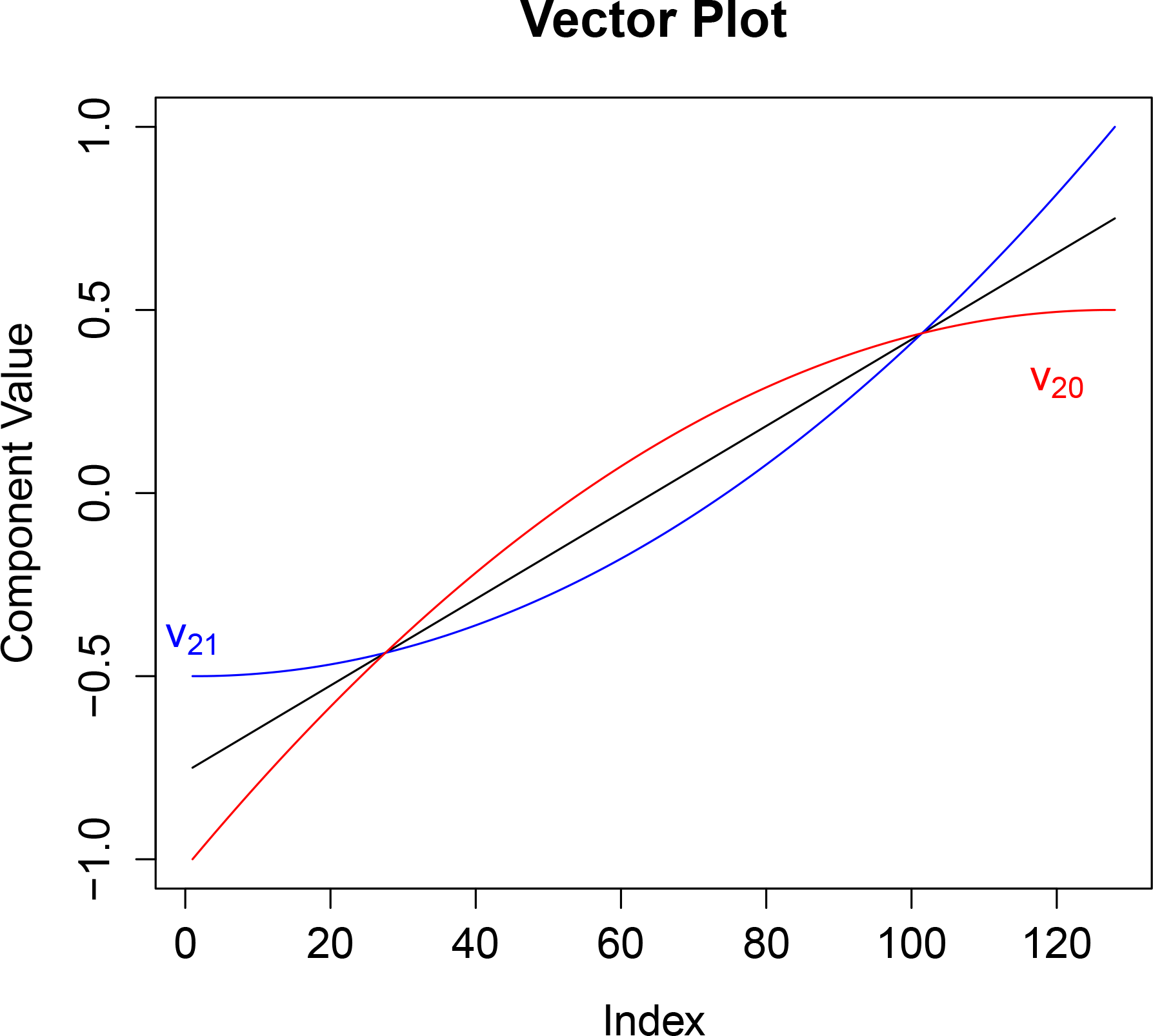
The second order vectors in Λ^↑ consists of the cone defined by the vectors v₂₀ and v₂₁ having components defined by

$$\begin{array}{l}(n-1){(v_{20})}^j=\frac{1}{2}j(j+1)-j-c_{20}\\ (n-1){(v_{21})}^j=-\frac{1}{2}j(j+1)+nj-c_{21}\end{array}$$

Notice that this cone contains v₁ since v₁ is proportional to v₂₀ + v₂₁. Many discrete one dimensional exponential families (e.g., binomial, negative binomial, and Poisson) use the vector v₁. Furthermore, many continuous one dimensional exponential families use the continuous function f used to define v₁: normal with σ known, and the gamma and inverse Gaussian distributions with known shape parameter (the shape parameter is the non-scale parameter). The cone defined by v₂₀ and v₂₁ allows us to perturb the v₁ direction to obtain related exponential families that we would expect to have similar properties. Figure 4 shows v₂₀ and v₂₁ as well as v₁ = 0.5v₂₀ + 0.5v₂₁.

Other vectors can be used to define cones around v₁. Looking at common exponential families we see that log(x) and x⁻¹ are sufficient statistics so that these suggest taking f̄(x) = log(x) or f̄ (x) =1/x. These can be further generalized to f̄ (x; λ), which can be the power family or some other family of transformations. The vectors v_f0 and v_f1 are defined using the discretized f with the constraints that v_f0, v_f1 ∈ Λ^↑ and 0.5v_f0 + 0.5v_f1 = v₁.

An exponential family with sufficient statistic x can be modified by choosing a function f̄ (x) and 0 ≤ α ≤ 1 where α = 0.5 corresponds to the original exponential family and other values perturb this direction. We denote this vector as v_fα so that v₀ + tv_fα is the natural parameter of the modified family.

Figure 4 shows the components of the vectors v₂₀ and v₂₁.

Since v₀ is common to each exponential family with natural parameter ℓ(t) = v₀ + tv_fα, the monotone likelihood ratio property will hold even if v₀ ∉ Λ^↑. Initial choices for v₀ are suggested by the Poisson, binomial, and negative binomial distributions:

$$\begin{array}{l}{(v_{\text{Poisson}})}^j=-\text{log}\Gamma (j)+c\hspace{0.17em}\hspace{0.17em}\hspace{0.17em}\hspace{0.17em}\hspace{0.17em}\notin {\Lambda }^{\uparrow }\\ {(v_{\text{binomial}})}^j=\text{log}\Gamma (n)-\text{log}\Gamma (j)-\text{log}\Gamma (n-j)+c\hspace{0.17em}\hspace{0.17em}\hspace{0.17em}\notin {\Lambda }^{\uparrow }\\ {(v_{\text{neg}.\text{bin}.})}^j=\text{log}\Gamma (j+r)-\text{log}\Gamma (j)+c\hspace{0.17em}\hspace{0.17em}\hspace{0.17em}\hspace{0.17em}\hspace{0.17em}\hspace{0.17em}\in {\Lambda }^{\uparrow }\end{array}$$

where c is a constant chosen so that the components sum to 1, n is the number of bins, and r is a positive real constant.