Speeding up Derivative Configuration from Product Platforms

Abstract
: To compete in the global marketplace, manufacturers try to differentiate their products by focusing on individual customer needs. Fulfilling this goal requires that companies shift from mass production to mass customization. Under this approach, a generic architecture, named product platform, is designed to support the derivation of customized products through a configuration process that determines which components the product comprises. When a customer configures a derivative, typically not every combination of available components is valid. To guarantee that all dependencies and incompatibilities among the derivative constituent components are satisfied, automated configurators are used. Flexible product platforms provide a big number of interrelated components, and so, the configuration of all, but trivial, derivatives involves considerable effort to select which components the derivative should include. Our approach alleviates that effort by speeding up the derivative configuration using a heuristic based on the information theory concept of entropy.
1. Introduction
To increase variety, improve customer satisfaction, reduce lead-times, and shorten costs, many companies have shifted from mass production to mass customization [1]. This shift of paradigm enriches the mass production economies of scale with custom manufacturing flexibility by developing families of related products instead of single products. From this perspective, designing a product family is the process of capturing and modeling multiple product variants to satisfy different market niches. A generic architecture, named product platform, is designed to support the creation of customized products called derivatives.
Product platforms usually support a high quantity of derivatives. For instance, the number of derivatives for product platforms in the automotive industry may range from 103 for the smallest Peugeot and Nissan car models, to 1016 or 1021 for the BMW 3-Series and Mercedes C-Class, respectively [2]. To achieve that flexibility, a number of configuration options are available. For example, the Peugeot 206 and Mercedes C-Class car models have 86 and 389 customer selectable options, respectively. Typically, not all option combinations are valid. There may be option incompatibilities (e.g.,“manual transmissions are not compatible with V8 engines”), option dependencies (e.g., “sport cars require manual gearbox”), etc. Configuring a valid derivative implies ensuring that all constraints between its constituent components are satisfied. Checking by hand those constraints is infeasible for all, but the most trivial product platforms, so derivative configuration is usually assisted by automated configurators [3]. Some examples of commercial configurators are Configit [4], SAP Product Configurator [5], Oracle Configurator [6], etc. In addition, many automotive companies have their own configurators. For instance, Volvo uses KOLA, Scania uses SPECTRA, Mercedes uses SMARAGD, etc.
Our work enriches existing configurators by reducing the number of steps required to configure a valid derivative. It takes advantage of the fact that, due to the component composition constraints, some decisions may be automatically derived from other decisions previously made. Therefore, the order in which decisions are made has a strong influence on the number of decisions required to complete a derivative. For instance, given the constraint “sport cars require manual gearbox”, a customer might configure a sport car using two decision orderings: one requiring two steps (i.e., Step 1, select “manual gearbox”, and Step 2, select “sport car”) or another one using just a single step (i.e., select “sport car”, so that the decision to select “manual gearbox” is implicitly made).
As van Nimwegen et al. [7] note, customers sometimes prefer to first answer questions that are important to them, or easy to answer, before being led through the remaining questions [7]. In this sense, our approach respects customer preferences. Instead of imposing a fixed ordering, it suggests orderings dynamically, reacting to the customer decisions. In particular, the process to get a derivative is performed in successive steps. In each step, the customer gets a question ranking, selects one of the questions and answers it. In the next step, the question ranking is readjusted to account for the customer’s answer. The computation of the ranking is grounded on the information theory concept of entropy, which was introduced by Shannon [8] and measures the average uncertainty of a random variable.
At the first configuration step, the uncertainty is total. With no information at all, the configurator cannot figure out which derivative the customer desires. As the process advances, configuration options are eliminated according to the customer decisions, and so, the information about the final configuration increases (i.e., the set of included/excluded components grows). Consequently, the entropy decreases. When the derivative is totally configured, there is no uncertainty, and the entropy is zero.
As we will see, not only our approach, but also Mazo et al.’s Heuristic 3 [9] and Chen et al.’s approach [10] require computing the probabilities of all variables in a Boolean formula. The usual way to perform such task is calling repeatedly a logic engine, e.g., a SATsolver or a binary decision diagram (BDD) library, one time for each variable [11]. Unfortunately, this approach has a high computational cost and, thus, imposes long response times, hindering customer-configurator interactivity. To overcome such a problem, this paper proposes an algorithm that computes efficiently variable probabilities using BDDs. Since more complex logics than the propositional one, which include integer arithmetic, transitive closure, etc., can be reduced to Boolean functions [12,13] and, thus, encoded as BDDs, our algorithm is general enough to support most configuration model notations.
The validity of our approach has been tested on two benchmarks widely used by the configuration and software product line communities: the Renault Megane platform provided by the car manufacturing company Renault DVI [14] and the Electronic Shopping case study [17]. Results show that our approach requires less configuration steps than related work, and that our BDD algorithm gets short response times, supporting this way not only our approach but also other methods proposed in related work.
The remainder of this paper is structured as follows. Section 2 presents the running example that we will use to motivate and illustrate our work. Section 3 summarizes related work to our approach. Section 4 introduces the concept of entropy and describes how to compute it from a configuration model. Later, our entropy-driven approach is described in detail. Section 5 reports the experimental validation of our approach. Finally, Section 6 outlines the conclusions of our work.
2. Motivational Example
This section illustrates the problem our approach tackles using an example provided by [18], where derivatives are cars with different automated driving capabilities.
To model the configurable options of a product family, a number of different notations are available. For instance, feature diagrams (FDs) [19], decision diagrams [20], the Configit language, the SAP Product Configurator language, the Oracle Configurator language, etc. Interestingly, most of those notations are semantically equivalent [21,22]. In fact, automated configurators instead of processing configuration models directly usually translate them into a propositional logic representation, such as a logic formula in conjunctive normal form, a BDD, etc. That logic representation is then processed using off-the-shelf tools, such as SAT solvers, BDD engines, etc. (see Section 4.1.2. for an explanation of the configuration model to logic translation). The input to our approach is the logic representation of the configuration model, so it is independent of the original notation used to specify the model.
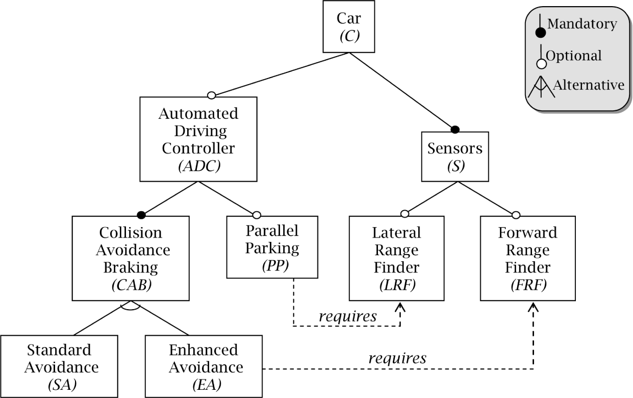
To show what a configuration model looks like, please refer to Figure 1, which models our running example as an FD (a hierarchically arranged set of features with different relations among them). This paper follows the generic semantics for FDs given by Schobbens et al. [22]. Figure 1 includes three kinds of hierarchical relations:
optional, denoted by simple edges ending with an empty circle; e.g., cars may (or may not) include an automated driving controller (ADC).
mandatory, denoted by simple edges ending with a filled circle; e.g., if a car has an ADC, it must include some kind of collision avoidance braking (CAB).
alternative, denoted by edges connected by an arc; e.g., standard avoidance (SA) and enhanced avoidance (EA) are the mutually exclusive options for collision avoidance braking (CAB).
To manage the complexity of modeling the similarities and differences among the derivatives of a product family, the FD notation follows a divide and conquer strategy. Derivative variabilities are modeled by progressively decomposing complicated and abstract features into simpler ones, until elemental features, which are directly implemented by physical components, are reached. The hierarchical structure of an FD graphically depicts such conceptual decomposition. From here on, derivatives will be expressed enumerating the final components they include, i.e., using references to the terminal nodes of the FD. For example, {PP, LRF, FRF, ¬SA, EA} expresses the configuration of a car with components PP, LRF, FRF, EA and without SA.
The FD notation supports narrowing the configuration space by adding additional cross-tree constraints. For instance, Figure 1 represents as the fact that cars with parallel parking need to include the lateral range finder component. Thus, a car derivative with components {PP, ¬LRF, ¬FRF, SA, ¬EA} complies with the FD relations, but is not valid because it violates the constraint .
For a configuration model with n options and no component interdependencies, the number of possible configurations is 2n. Due to the feature relations and additional cross-tree constraints, the number of valid configurations in the example is reduced from 25 = 32 to the 13 ones summarized in Table 1.
To configure a car, the decision-maker needs to answer a sequence of questions. For example, the sequence (1) is EA in the configuration? no, (2) FRF? no, (3) LRF? yes, (4) PP? yes configures Car 11 in Table 1. Current automated configurators guarantee the derivation of valid products ensuring the satisfaction of all model constraints. When the first question is answered, the configurator deduces that the car being configured necessarily includes SA (otherwise, the alternative relation between EA and SA would not hold). This way, the configurator is indirectly saving the decision-maker from answering the irrelevant question, “is SA in the configuration?”
The goal of our work is to make the most of the configuration model constraints going beyond current configurators to minimize the number of questions required to specify a derivative. To do so, our approach tries to find an optimal question ordering that maximizes the number of decisions automatically derived from other questions previously answered.
A straightforward approach to get such optimal question ordering is computing for each valid product all possible orderings and, thus, finding the ordering with less questions on average for every product. Table 2 sums up the needed computations. For instance, the next-to-last column summarizes the number of questions needed for derivative {PP, LRF, FRF, SA, ¬EA}. Ordering PP ≺ LRF ≺ FRF ≺ SA ≺ EA needs three questions, LRF ≺ PP ≺ FRF ≺ SA ≺ EA needs four, and so on. Afterwards, the average number of questions for each ordering is computed. Using this approach in the previous example, ordering PP ≺ LRF ≺ FRF ≺ SA ≺ EA would be selected as an optimal one. As a result, the question sequence for Derivative 11 in Table 1 would be shortened to (1) is PP in the configuration? yes, (2) FRF? no, (3) SA? yes, removing the need for answering “if LRF is in the configuration”.
Unfortunately, this approach requires m · n! computations, where n is the number of components of the configuration model and m is a number ≤ 2n. Therefore, it is extremely expensive in computational terms and does not scale, except for the most trivial configuration models. To overcome the scalability limitations of the former approach, this paper proposes a heuristic solution grounded on the information theory concept of entropy.
3. Related Work
Research on automated configurators is mainly focused on consistency checking and optimization [3,23]. For example, reasoning engines, such as BDD libraries, SAT solvers and logic-truth maintenance systems, have been used to detect invalid derivatives (i.e., those which violate some option dependency or incompatibility) [24–26], to provide explanations for configuration flaws [27,28], to optimize configurations (i.e., to find configurations whose cost is less or equal than a given one) [29–31], etc.
Despite the importance of the interactive question ordering problem that our work tackles, which was pointed out by Steinberg more than thirty years ago [32], there is little research on it. A recent approach that specifically deals with this problem is provided by Chen et al. [10], who propose to minimize the number of configuration steps by sorting the components according to their probability of being included in a derivative. Such a probability is computed by Equation (1).
In their original paper and with a fully equivalent meaning, Chen et al. [10] use the term selectivity instead of probability. As our approach follows an entropy driven heuristic and the information theory concept of entropy is defined in terms of probability (see Section 4.1.1.), we have preferred to use probability throughout this paper.
In addition to Chen et al.’s approach, Mazo et al. [9] proposes the following heuristics for ordering configuration questions:
Heuristic 1: Components with the smallest domain first. Choose first the component with the smallest domain. The domain of a component is the set of possible values that the component can take according to its domain definition and the constraints in which the component is involved.
Heuristic 2: The most constrained components first. Choose the component that participates in the largest number of constraints.
Heuristic 3: Components appearing in most products first. This heuristic is exactly the same as Chen et al’s approach.
Heuristic 4: Automatic completion when there is no choice. This heuristic “provides a mechanism to automatically complete the configuration of variables where only one value of their domain is possible […] it also works when a variable has several values on its domain but only one is valid”. In ascending order of computational cost and descending order of constraint propagation capacity, Mazo et al. [9] summarize three approaches to implement Heuristic 4 when the configuration model is encoded as a predicate logic formula: (i) forward-checking; (ii) partial look-ahead; and (iii) full look-ahead (i.e., whereas forward-checking is the fastest algorithm, but produces the most limited form of constraint propagation during search, full look-ahead is the most expensive approach, but gets the best results). In our paper, configuration models are encoded as propositional logic formulas, where a full constraint propagation is computationally feasible. In particular, a configuration model will be encoded as a BDD ψ. To completely propagate a customer decision d, the BDD ψ ∧ d will be computed. Fortunately, this computation only takes linear time on the size of the BDD. That is, the complexity of computing mixing two BDDs ψ1 and ψ2 using the apply algorithm proposed by Bryant [33] is O(|ψ1||ψ2|), so the complexity of ψ ∧ d is O(|ψ||d|) = O(|ψ| · 1) = O(|ψ|). Instead of considering Heuristic 4 apart, we will use it as a complement to the remaining heuristics by running constraint propagation after every configuration step.
Heuristic 5: Components required by the latest configured component first. Choose the component that has the largest number of constraints with the past-configured components.
Heuristic 6: Components that split the problem space in two first. Set first the components that divide the problem space into two parts of approximately the same size. Unfortunately, Mazo et al. [9] do not provide a way to implement this heuristic, which takes into account all model constraints. In particular, Mazo et al. propose a simplification by just using the tree structure of an FD, or the variation points of an orthogonal variability model [34], but not processing the cross-tree constraints.
As will be discussed in Section 4.3, our approach may be thought of as an implementation of Heuristic 6 that, in addition, takes into account all configuration model constraints. In Section 5, it will be shown that our approach provides better outcomes than Heuristics 1, 2, 3 (i.e., Chen’s approach [10]) and 5.
4. Entropy-Based Approach to Sort Configuration Questions
This section presents our heuristic to minimize the number of steps required to configure a derivative from a configuration model. Section 4.1.1. introduces the theoretical background of our approach. As we will see, our heuristic, as other ones summarized in Section 3, requires computing the component probabilities. Section 4.1.2. discusses the scalability limitations of the approach commonly used to compute those probabilities. To overcome such limitations, in Section 4.2, we propose an algorithm that provides an efficient probability computation. Finally, Section 4.3 describes our heuristic.
4.1. Preliminaries
4.1.1. Information Theory
The following definitions were originally introduced by Shannon [8]. Let us start with the concept of entropy.
Definition 1 Let X be a discrete random variable with alphabet and probability mass function; the entropy H of X is defined by Equation (2):
Let us present the concept of conditional entropy, which is the entropy of a random variable conditional on the knowledge of another random variable.
Definition 2 Let X and Y be two discrete random variables. The conditional entropy H(X|Y) of X given Y is defined by Equation (3):
Finally, let us introduce the concept of mutual information, also called information gain, which represents the reduction in a variable uncertainty due to another random variable.
Definition 3 Consider two random variables Xand Ywith a joint probability mass function Pr(x, y) and marginal probability mass functions Pr(x) and Pr(y). The mutual information I(X; Y) is defined by Equation (4) as the relative entropy between the joint distribution and the product distribution Pr(x)Pr(y):
Entropy and mutual information satisfy the following properties that will be used throughout this paper:
- (1)
H(X) ≥ 0
- (2)
, with equality if and only if X is distributed uniformly over (in this paper, the number of elements of a set S is denoted as #S)
- (3)
I(X; Y) = H(X) − H(X|Y) = H(Y) − H(Y|X) = I(Y; X)
4.1.2. Straightforward Approach to Compute Component Probabilities
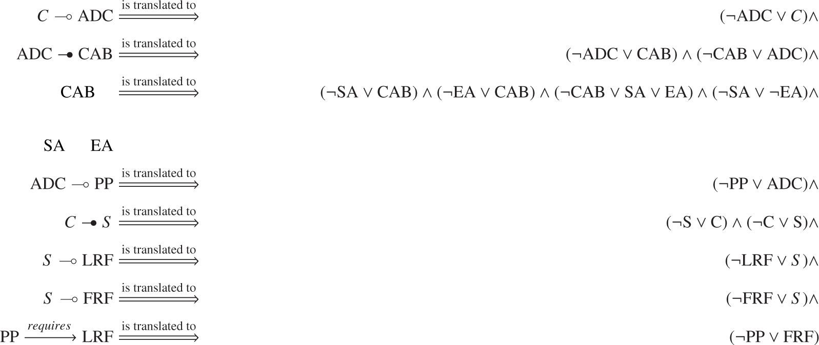
A widespread approach to support the automated management of configuration models is translating them to propositional logic formulas [3,25], which are processed using off-the-self tools, such as SAT solvers [35] or BDD engines [33]. Table 3 summarizes the translations needed to encode our running example into propositional logic. A more detailed explanation of how to translate feature models into logic may be found in [36]. Equation (5) is the equivalent logic formula to Figure 1.

Once a configuration model is encoded into a logic formula ψ:
the total number n1 of valid derivatives is equivalent to the number of satisfying assignments of ψ (i.e., those that evaluate ψ to be true).
the number n2 of valid derivatives that include component c is equivalent to the number of satisfying assignments of ψ ∧ c.
Since the probability of a component is and the computation of the number of satisfying assignments of a Boolean formula is supported by most BDD engines and SAT solvers (in particular, #SAT counters are a type of SAT solver specifically oriented to compute such a number), a straightforward approach to compute the component probabilities is calling repeatedly a logic engine using ψ ∧ ci as the input [11]. Unfortunately, this approach has a high computational cost and does not scale for all, but trivial configuration models. While the SAT problem is known to be NP-complete [37], it is widely believed that the #SAT problem is even harder [35]. If n is the number of components, computing the component probabilities requires calling a #SAT solver n times, which is extremely time-consuming. Similarly, computing the number of satisfying assignments with a BDD has computational complexity O(m) [33], where m is the number of nodes of the BDD. Hence, the complexity of computing the component probabilities by calling repeatedly the BDD engine is O(n · m), which is excessively time-consuming for most configuration models.
For instance, it is well known by the car manufacturing community that the first issue of car configurators is performance [38]. Thus, as soon as customers make a configuration choice, they want to find out what the consequences of the choice are. From a marketing perspective, it is unpleasant for customers to wait for several seconds to know whether their requirements are correct or not in terms of configuration. As it will be shown experimentally in Section 5, computing the component probabilities by calling repeatedly a BDD may force the costumer to wait for more than 600 seconds for just a single configuration step!
To overcome the aforementioned scalability limitations, in the following section, we propose a BDD algorithm that computes component probabilities in almost linear time to m.
4.2. Efficient Computation of the Probabilities of the Variables of a Boolean Formula from a BDD
BDDs are a way of representing Boolean functions. They are rooted, directed, acyclic graphs, which consist of several decision nodes and terminal nodes [33]. There are two types of terminal nodes, called 0-terminal and 1-terminal. Each decision node vi is labeled by a Boolean variable xk and has two child nodes called low and high (which are usually depicted by dashed and solid lines, respectively). The edge from node vi to a low (or high) child represents an assignment of vi to 0 (resp. 1). Such a BDD is called ordered if different variables appear in the same order on all paths from the root. A BDD is said to be reduced if the following two rules have been applied to its graph: (i) isomorphic subgraphs are merged; and (ii) nodes whose two children are isomorphic are eliminated.
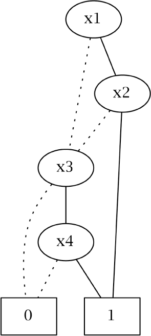
In popular usage, the term BDD almost always refers to a reduced ordered binary decision diagram [12]. In this paper, we will follow that convention, as well. Let us use formula ψ ≡ (x1 ∧ x2) ∨ (x3 ∧ x4) as a running example for this subsection. Table 4 is the truth table for ψ. Figure 2 is its BDD representation using the variable ordering x1 ≺ x2 ≺ x3 ≺ x4. Note that a logic formula may be encoded with different BDDs according to the variable ordering used to synthesize the BDD. Obviously, our algorithm produces the same results for equivalent BDDs (i.e., BDDs that encode the same formula).
The remainder of this subsection is structured as follows. Firstly, some definitions required to understand our algorithm are given. Next, the data structures that the algorithm uses are described from a theoretical perspective. Then, the algorithm is presented. Finally, the algorithm computational cost is discussed.
4.2.1. Definitions
Definition 4 The satisfying set of a Boolean formula ψ(x1,…, xn), denoted Sψ, is defined by Equation (6).
Definition 5 The satisfying set of the variable xi of a Boolean formula ψ(x1,…, xi−1, xi, xi+1,…, xn), denoted, is defined by Equation (7).
For instance, according to Table 4, #Sψ = 7 since there are seven rows where ψ evaluates as true (throughout this paper, 0/1 and false/true are used interchangeably), and , because x4 = 1 in five of the seven rows where ψ = 1.
Definition 6 The satisfying probability of a Boolean formula ψ(x1,…, xn), denoted Pr(ψ), is defined by Equation (8).
Definition 7 The satisfying marginal probability of a variable xi in a Boolean formula ψ(x1,…, xi−1, xi, xi+1,…, xn), denoted, is defined by Equation (9).
Definition 8 The satisfying probability of a variable xi in a Boolean formula ψ(x1,…, xi−1, xi, xi+1,…, xn), denoted, is defined by Equation (10).
For instance, looking at Table 4, it is easy to see that , and . For convenience, in the remainder of the paper, we denote and
as Pr(xi) and MPr(xi), respectively.
4.2.2. Data Structures
Let us represent a BDD that has m nodes and encodes a Boolean formula with n variables by using the following data structures:
The variable ordering used to synthesize the BDD is represented by an array declared as follows:
var_ordering: array[0..n-1] of string
Each node is represented by a record declared as follows:
type node = record
index: 0..n
low, high: node
mark: Boolean
end
where:
- (1)
index is the index of the variables in the ordering. The terminal nodes of the BDD (i.e., 0 and 1) have index n.
- (2)
low and high are the low and high node successors
- (3)
mark is used to mark which nodes have been visited during a traversal of the graph. As we will see, our algorithm is called at the top level with the root node as the argument and with the mark fields of the nodes being either all true or all false. It then systematically visits every node in the graph by recursively visiting the subgraphs rooted by the two children, low and high. As it visits a node, it complements the value of the mark field, so that it can later determine whether a child has already been visited by comparing the two marks.
The BDD is represented by an array declared as follows:
bdd: array[0..m] of node
The terminal nodes of the BDD, 0 and 1, are stored at Positions 0 and 1 of the bdd array, respectively.
For instance, Tables 5 and 6 represent the content of bdd and var_orderingfor the BDD in Figure 2, respectively.
4.2.3. Algorithm
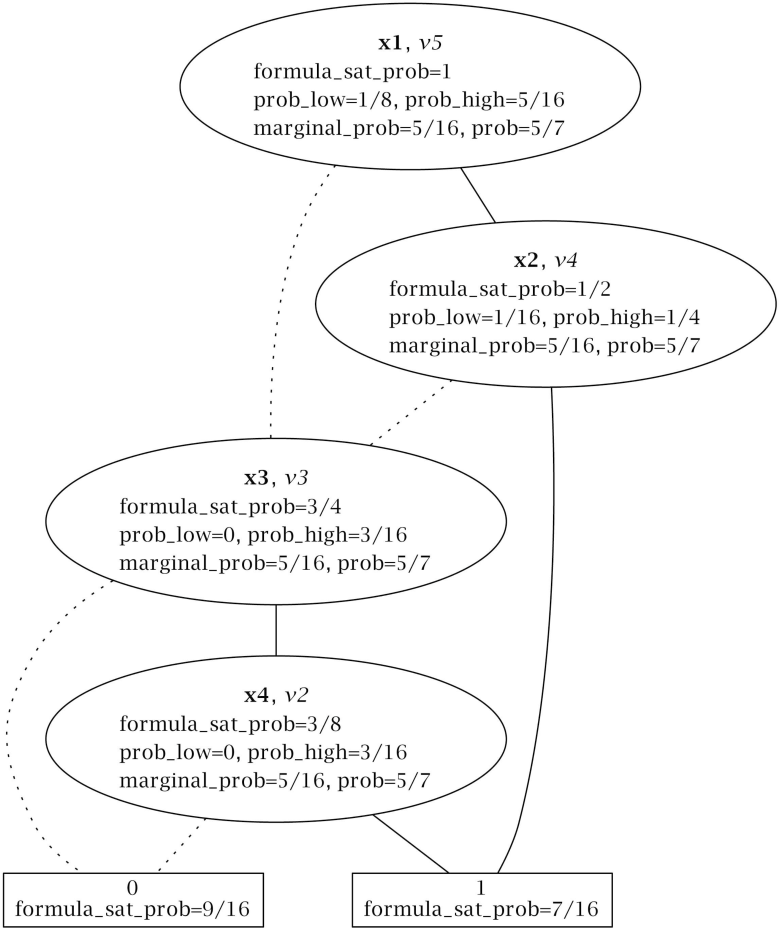
Pr(xi) is computed jointly by Algorithms 1, 2 and 3. Figure 3 summarizes the computations for the BDD in Figure 2. Let us examine how our approach proceeds:
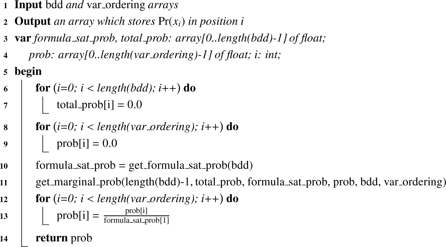
Algorithm 1 computes Pr(xi) as by calling the auxiliary Algorithms 2 and 3.
Algorithm 2 computes Pr(ψ).
A nice mental picture to understand Algorithm 2 is thinking about pouring one liter of water from the BDD root to the terminal nodes. One liter goes through the root, then half a liter goes through the low branch and half a liter through the high branch. This procedure advances, until the water reaches the leaves. Hence, MPr(xi) is the amount of water that Node 1 has.
According to Tables 5 and 6, the root node has label v5, and it is in Position 5 of the bdd array. In Figure 2, through node v5 goes one liter (i.e., formula_sat_prob[5] = 1). Half of it goes to v3 and the other half to v4. Whereas, through v4 passes liters, through v3 goes the liters that come from v5 and half of the water that comes from v4.
Algorithm 3 computes MPr(xi).
In particular, let us examine how it computes MPr(x2). In the truth Table 4, ψ evaluates as true when x2 is true five times:
In four of them, x1 is true. When the call get_marginal_prob(4, …) is made, Lines 10–23 compute the marginal probability of x2 for the explicit path v5 → v4. The probabilities due to the low and high branches of vi are stored into the prob_low and prob_high variables, respectively. As bdd[4].low ≠ 0, a recursive call is made to compute the total probability due to the low descendants of v4 (i.e., get_marginal_prob(3, …)). As a result:
Notice that is not simply equal to total_prob[3], because total_prob[3] depends also on the probability that comes from the link v5 ⤏ v3. To get just the probability due to the link v4 ⤏ v3, prob_low has to be adjusted using the formula_sat_prob array as:Since bdd[4].high = 1, prob_high is directly computed as:Finally:In one of them, x1 is false. The two following implicit paths have been removed from the reduced BDD, (i) v5 ⤏ v4 ⤏ v3; and (ii) v5 ⤏ v4 → v3. Nevertheless, path v5 ⤏ v4 → v3 should be considered to compute the marginal probability of x2. Lines 24–31 account for that kind of implicit path, adjusting the marginal probability with the variables omitted in the paths. For instance, when the algorithm is called for v5, the marginal probability of x2 is updated with half the prob_low of v5.
To sum up:
![Entropy 16 03329f9]()
4.2.4. Computational Cost
Let m be the number of nodes of the BDD and n the number of variables of the Boolean formula. Algorithm 2 requires traversing all of the nodes, so its computational complexity is O(m). Algorithm 3 also traverses all of the BDD nodes. In addition, to account for the implicit paths removed from the reduced BDD, the variables omitted on the edges that come from each node need to be traversed (which is done by Lines 24–31). Table 7 summarizes those traversals for Figure 2. For instance, when v4 is recursively traversed, the variables x3 and x4 need to be iteratively traversed, because the edge v4 → 1 omits them (i.e., the variable encoded by node v4, x2, jumps directly to one, omitting the intermediate variables x3 and x4 in the ordering x1 ≺ x2 ≺ x3 ≺ x4). Table 7 helps with noticing the savings our algorithm provides compared to the straightforward approach described in Section 4.1.2., which requires traversing all nodes for all variables (which in computational cost terms is equivalent to traversing all variables for every node). Therefore, Algorithm 3 does not traverse m · n elements, but m · n′, where n′ is strictly less than n. Otherwise, if n′ = n, all nodes in the BDD should go directly to zero or one, jumping over all of the variables. Nevertheless, as BDDs are organized in hierarchical levels according to the variable ordering, this is impossible (i.e., the nodes that encode a variable with position k in the ordering can only jump over the variables with positions k + 1 …n).
It follows that Algorithm 1 has computational complexity O(m · n′). As will be shown in Section 5, in practice, n′ is usually much smaller than n, and thus, variable probabilities can be efficiently computed.
4.3. Entropy-Driven Configuration
Let us return to the original problem this paper tackles. Given a set of questions Q, our goal is to sort it in such a way that the user has to answer as few questions as possible to complete the configuration. To find the optimal order of Q, we propose to rank each question, q, according to its expected information gain, i.e., measuring how much uncertainty can be reduced on average when the engineer answers it. Such an information gain is modeled as the mutual information I(C; q), where C is the set of all valid configurations (i.e., the ones that satisfy all asset interdependencies).
When a configuration is completed, the entropy of every question q is zero. Since q has been answered, H(q|C) = 0. Thus, it follows that I(C; q) = H(q), as Equation (11) demonstrates (see Property 3 in Subsection 4.1.1.).
When we ask “is component c in the configuration?”, the entropy of the question H(q) is computed by Equation (12), where Pr(c) is the probability that c is included in the configuration.
Our approach to guide the configuration of a derivative may be thought of as a binary search for the user-desired configuration (remember Heuristic 6 in Section 3). To successively divide the search space into subspaces of approximately the same size (i.e., where the pursued configuration is approximately of the same probability), the user answers the question that provides more information about the configuration (i.e., the question with the highest entropy). Thus, the configuration process advances iteratively, by performing the following activities, until the entropy of all components becomes zero:
- (1)
Computing the component probabilities from the input configuration model. As the process advances, the configuration space gets narrower and, consequently, the component probabilities change.
- (2)
Computing the entropy value for each question.
- (3)
Sorting the questions in descending order of entropy.
- (4)
Asking the user to answer a question with entropy greater than zero. Note than when a question has zero entropy, it is because it has been answered in a previous step directly or indirectly (i.e., because of the question interdependencies).
- (5)
Updating the set of answers and the configuration model (e.g., if the customer answers a question q negatively, the Boolean formula ψ that encodes the configuration model is updated to ψ ∧ ¬ f).
Entropy may also be used to measure how hard it is to configure a given model. From the “point of view” of an automated configurator, when the configuration process starts, the derivative desired by the customer is any c in C with the same probability. Therefore, the configuration model uncertainty is calculated by Equation (13) (see Property 2 in Section 4.1.1.).
4.3.1. Example
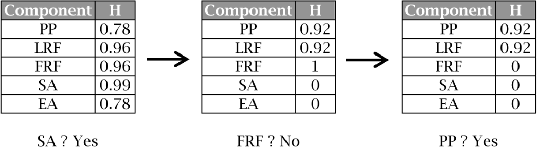
Coming back to the running example introduced in Section 2, let us see how our approach works. Figure 4 sums up the steps required to configure the derivative {PP, LRF, ¬FRF, SA, ¬EA} using the entropy heuristic. In the first step, EA is the component with the highest entropy. Therefor, the system asks the user if SA is included in the derivative. Once the user answers affirmatively, the probabilities of the components are recomputed and, so, the entropies (e.g., the inclusion of SA implies the exclusion of EA, so Pr(EA)=0 and thus H(EA)=0).
We remark here that our approach does not force the user to follow a fixed sequence of questions. In each configuration step, the user may decide not to answer the best entropy-ranked question, but the one she thinks is more convenient. After the question is answered, the entropies are recomputed and, thus, our approach adjusts to the user preferences in an interactive way.
5. Experimental Evaluation
To test the validity of our approach, we have used two case studies:
- (1)
The configuration model provided by the car manufacturing company Renault DVI [14], which deals with the configuration of a family of cars named Renault Megane and is freely available at [15]. We have selected this model because it illustrates the practical applicability of our approach (i.e., instead of using an example made up for academic purposes, our work is tested on a real configuration model that comes from the industry). In addition, the Renault Megane problem is a benchmark of widespread use by the configuration community [39–49].
- (2)
The Electronic Shopping model provided by Lau [17], which deals with an electronic commerce platform that allows consumers to directly buy goods or services from a seller over the Internet using a web browser. This benchmark is widely used by the software product line community [26,50,51] and is freely available at [16].
5.1. Experimental Design
The goal of this section is to check if:
Our approach produces better results than related work.
The algorithm presented in Section 4.2 provides reasonable response times and, thus, supports customer interactivity during the configuration process.
To do so, we have created a test bed composed of 1,000 random derivatives for every configuration model. As we will see, a sample of 1,000 derivatives is big enough to get results with high statistical power and significance.
To generate valid derivatives that satisfy all constraints, we have encoded the models as propositional logic formulas (see Subsection 4.1.2.) and then as BDDs. To get efficient BDD sizes, the directions given by Narodytska et al. [43] have been followed. The BuDDy package [52] has been used to guarantee the generation of valid derivatives (i.e., derivatives that conform to the BDD).
The test bed is used to compare the following methods:
- (1)
Mazo et al.’s Heuristics 1, 2 and 5. [9] Remember that, strictly speaking, Mazo et al.’s Heuristic 4 is not a heuristic, but a propagation mechanism that all configuration systems should support. Therefore, we have included such mechanism in all of the methods tested in this paper.
- (2)
The probability-driven approach, i.e., the method proposed by Chen et al. [10] and Mazo et al. [9] (Heuristic 3).
- (3)
The entropy-driven approach, i.e., the method we propose in this paper.
To compute the option probabilities, which are required by the entropy and probability approaches, an implementation of the algorithm presented in Section 4.2 has been included into the BuDDy package.
5.2. Case Study 1: Renault Megane
5.2.1. Results
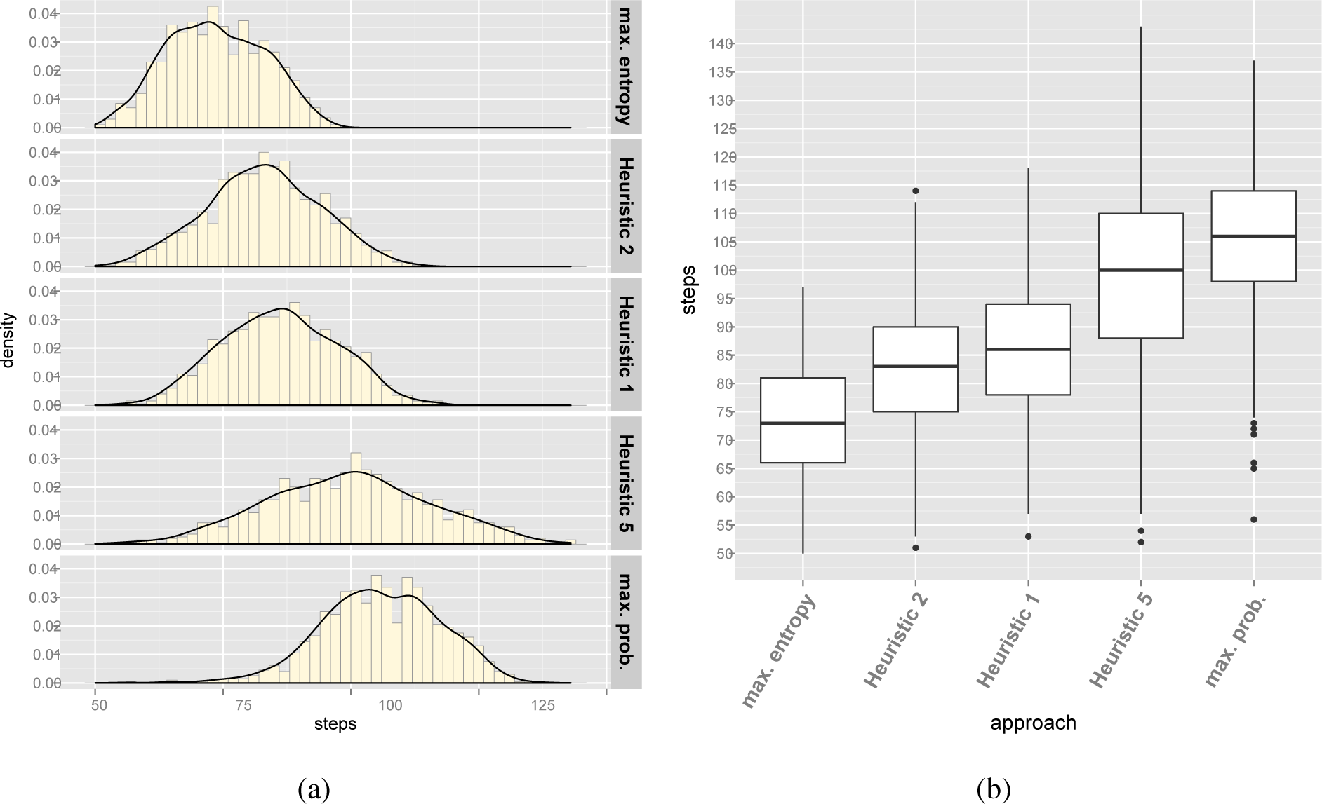
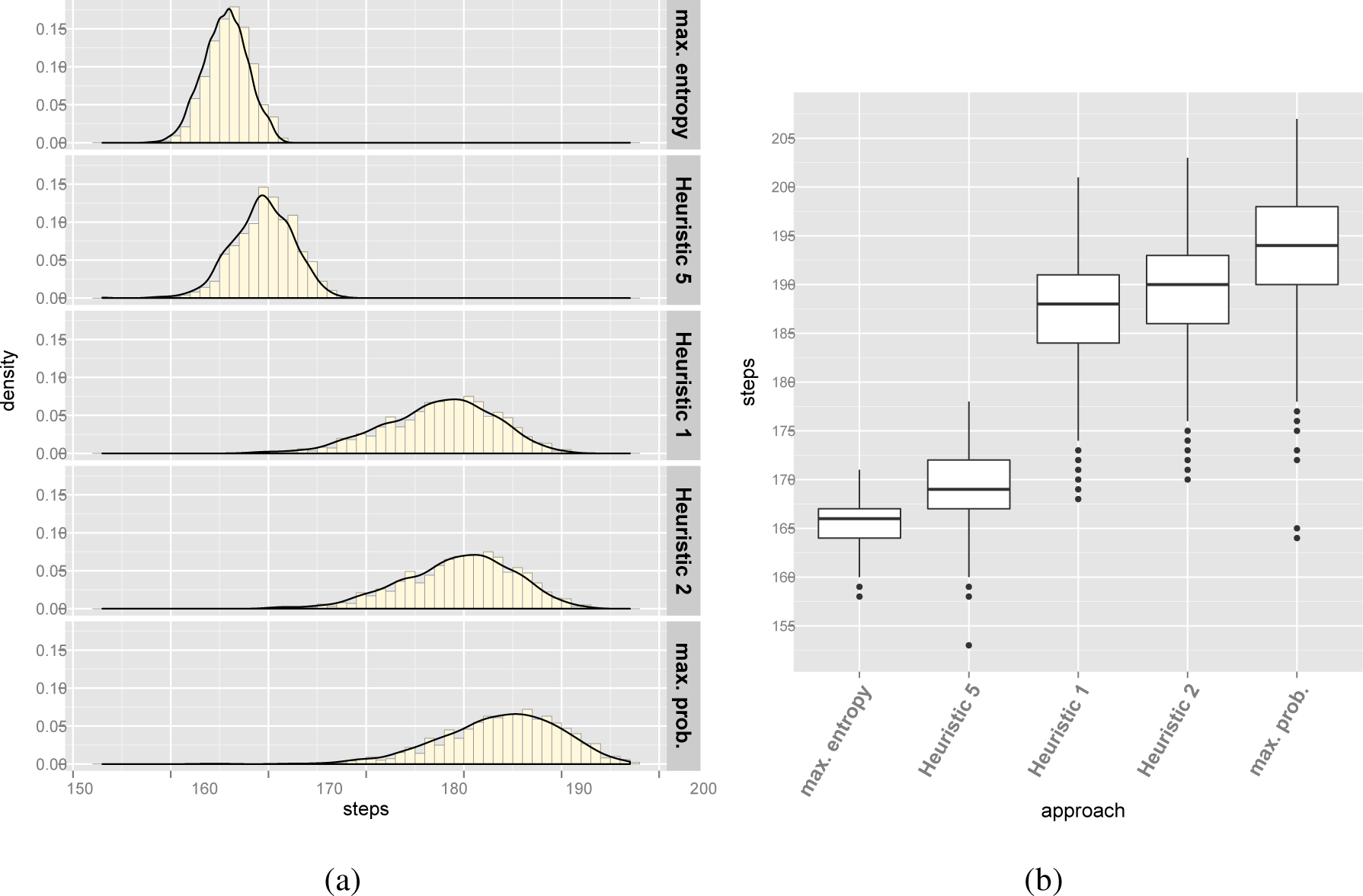
Table 8 summarizes the results of the experiments for the Renault Megane configuration model. Histograms in Figure 5a represent the number of steps needed to configure the 1,000 derivatives using Mazo et al.’s [9] Heuristics 1, 2 and 5 and the entropy and probability approaches. Figure 5b complements the histogram representation of the results with a box plot. In Figure 5b, “whiskers” start from the edge of the box and extend to the furthest data point that is within 1.5 times the inter-quartile range (i.e., the range that goes from the 25th percentile to the 75th percentile). Points that are past the ends of the whiskers have been considered outliers and are displayed with dots.
Using the central limit theorem, the 95% confidence intervals (CI) of the population mean can be estimated (i.e., the range where, with a 95% guarantee, the mean of the number of steps required to configure every derivative of the Megane model lies). Table 9 summarizes the CIs for each approach, which are estimated as population mean CI = sample mean±t(std. error, 95%, 999 degrees of freedom), where t stands for the Student’s t-distribution.
According to the summarized data, there is experimental evidence supporting that our approach produces better results than related work.
5.2.2. Statistical Significance
To check the statistical significance of the results, an analysis of variance (ANOVA) test has been run on the experimental data. Table 10 summarizes the ANOVA outcomes. Since the p-value is less than 0.001 (in particular, p-value < 2 · 10−16), the experimental results are statistically highly significant.
Table 11 summarizes the power analysis of the ANOVA test. Given the sample size and the high effect size (i.e., the high values of η2 and Cohen’s f2), the ANOVA test has high statistical power.
Finally, to check the statistical significance of the pairwise comparison between the approaches, a Tukey Honest Significant Differences (HSD) has been run. According to the results, summarized in Table 12, the difference between the number of steps required by any pair of approaches to configure a derivative is statistically highly significant. Whereas the ANOVA test rejects the null hypothesis: “there is no difference between the five approaches (i.e., all of them produce approximately the same results)”, the Tukey HSD test rejects ten null hypotheses separately: “there is no difference between Heuristic 2 and the entropy approach”, “there is no difference between Heuristic 1 and the entropy approach”, etc.
5.3. Case Study 2: Electronic Shopping
Table 13 and Figure 6 summarize the results of the experiments for the Electronic Shopping configuration model. Table 14 summarizes the CIs for each approach. According to the outcomes, there is experimental evidence supporting that our approach produces better results than related work.
5.3.1. Statistical Significance
Table 15 summarizes the ANOVA outcomes. Since the p-value is less than 0.001 (in particular, p-value < 2 · 10−16), the experimental results are statistically highly significant. Table 16 summarizes the power analysis of the ANOVA test. Given the sample size and the high effect size, the ANOVA test has high statistical power. Finally, Table 17 summarizes the outcomes of HSD, which show that the difference between the number of steps required by any pair of approaches to configure a derivative is statistically highly significant.
5.4. Threats to Validity
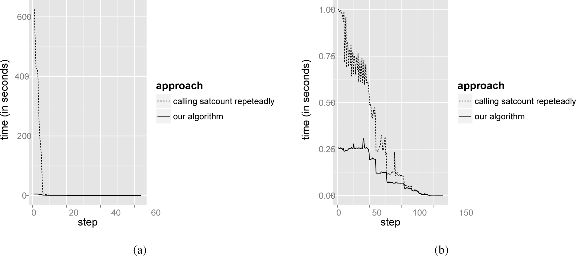
A threat to the validity of our approach is the time required to compute the component probabilities, which is also the Achilles’ heel for Chen et al.’s [10] approach and Mazo et al.’s [9] Heuristic 3. For the sake of interactivity, configurators must provide customer guidance in a short time, and the usual way to compute the probabilities is highly time consuming (see Section 4.1.2.). To assess the response time of our algorithm (see Section 4.2), we determined the time needed to configure 1,000 randomly generated derivatives for Case Studies 1 and 2 using our entropy-driven approach. Figure 7 compares the average times needed to completely configure the derivatives by computing the component probabilities using our algorithm and calling repeatedly the BuDDy function, satcount. The performance tests were conducted on an Intel©Core™ 2 i3-4010U with 1.7 GHz and 4GB RAM (although, only one core was used).
As Figure 7 shows, our algorithm greatly improves the probability computation time. For instance, it requires 4.54 seconds on average to compute all component probabilities (and thus, their entropy values) for the first configuration step in the Renault Megane example. In contrast, calling satcountrepeatedly consumes 625.18 seconds.
Note that the first configuration’s steps are the most expensive in time. As the configuration process advances, the configuration space gets reduced and, so, the time needed to compute the probabilities. There is a point where both approaches converge and get response times close to zero.
6. Conclusions
To satisfy a wide range of customers, product platforms must provide a high variety of optional components. For this reason, the configuration of all, but trivial, derivatives involves considerable effort in selecting which components they should include, while avoiding violations of the inter-component dependencies and incompatibilities. Our approach enriches existing automated configurators by reducing the number of steps required to configure a valid derivative.
Applying the information theory concept of entropy, our approach takes advantage of the fact that, due to the inter-component constraints, some decisions may be automatically derived from other decisions previously made. Therefore, the order in which decisions are made has a strong influence on the number of decisions required to complete a configuration. Moreover, our approach does not provide a static ordering that the customer is forced to follow. On the contrary, it suggests orderings dynamically, reacting to the customer decisions. In addition, we have proposed an algorithm that efficiently computes the variable probabilities of a Boolean formula, supporting in this way not only our approach, but also other methods proposed in related work.
The Renault Megane and Electronic Shopping configuration benchmarks have been used to test the applicability of our approach and its effectiveness. In particular, it has been shown that our approach needs less configuration steps than related work.
Acknowledgments
This work has been supported by the Spanish Government under the CICYT project DPI-2013-44776-R, and the Comunidad de Madrid under the RoboCity2030-II excellence research network S2009DPI-1559.
Author Contributions
This is a joint effort based on an original idea conceived by Ruben Heradio and David Fernandez-Amoros. The development of the idea, its implementation and validation has been performed by Ruben Heradio, David Fernandez-Amoros, Hector Perez-Morago, and Antonio Adan.
Conflicts of Interest
The authors declare no conflict of interests.
References
- Simpson, T.W.; Siddique, Z.; Jiao, J.R. Product Platform and Product Family Design: Methods and Applications; Springer: Berlin/Heidelberg, Germany, 2005. [Google Scholar]
- Pil, F.K.; Holweg, M. Mitigating product variety’s impact on the value chain. Interfaces 2004, 34, 394–403. [Google Scholar]
- Sabin, D.; Weigel, R. Product Configuration Frameworks-A Survey. IEEE Intell. Syst 1998, 13, 42–49. [Google Scholar]
- Configit, Available online: http://www.configit-software.com/ (accessed on 16 June 2014).
- SAP Product Configurator, Available online: https://scn.sap.com/docs/DOC-25224 (accessed on 16 June 2014).
- Oracle Configurator, Available online: http://docs.oracle.com/cd/B12190_11/current/acrobat/115czinstg.pdf (accessed on 16 June 2014).
- Van Nimwegen, C.; Burgos, D.; van Oostendorp, H.H.; Schijf, H. The paradox of the assisted user: Guidance can be counterproductive, Proceedings of the SIGCHI Conference on Human Factors in Computing Systems, Montreal, Canada, April 2006; ACM: New York, NY, USA, 2006; pp. 917–926.
- Shannon, C.E. A mathematical theory of communication. Bell Syst. Tech. J 1948, 27, 379–423. [Google Scholar]
- Mazo, R.; Dumitrescu, C.; Salinesi, C.; Diaz, D. Recommendation heuristics for improving product line configuration processes. In Recommendation Systems in Software Engineering; Springer-Verlag: Berlin/Heidelberg, Germany, 2014. [Google Scholar]
- Chen, S.; Erwig, M. Optimizing the Product Derivation Process, Proceedings of the 15th International Software Product Line Conference, Munich, Germany, 21–26 August 2011; IEEE Computer Society: Munich, Germany, 2011; pp. 35–44.
- Kübler, A.; Zengler, C.; Küchlin, W. Model Counting in Product Configuration, Proceedings of the 1st International Workshop on Logics for Component Configuration, Edinburgh, UK, 10 July 2010; pp. 44–53.
- Huth, M.; Ryan, M. Logic in Computer Science: Modelling and Reasoning about Systems; Cambridge University Press: Cambridge, UK, 2004. [Google Scholar]
- Jackson, D. Software Abstractions: Logic, Language, and Analysis, 2nd ed; The MIT Press: Cambridge, MA, USA, 2012. [Google Scholar]
- Renault DVI, Available online: http://www.renault.fr/ (accessed on 16 June 2014).
- Configuration Model of the Renault Megane Platform, Available online: http://www.itu.dk/research/cla/externals/clib/ (accessed on 16 June 2014).
- SPLOT: Software Product Lines Online Tools, Available online: http://gsd.uwaterloo.ca:8088/SPLOT/index.html (accessed on 16 June 2014).
- Lau, S.Q. Domain Analysis of E-Commerce Systems Using Feature-Based Model Templates. Master’s thesis, University of Waterloo, Waterloo, ON, Canada, 2006. [Google Scholar]
- White, J.; Dougherty, B.; Schmidt, D.C.; Benavides, D. Automated reasoning for multi-step feature model configuration problems, Proceedings of the 13th International Software Product Line Conference, San Francisco, USA, 24–28 August 2009; Carnegie Mellon University Press: Pittsburgh, USA, 2009; pp. 11–20.
- Kang, K.; Cohen, S.; Hess, J.; Novak, W.; Peterson, S. Feature-Oriented Domain Analysis (FODA) Feasibility Study; Technical Report CMU/SEI-90-TR-21; Software Engineering Institute: Pittsburgh USA, 1990. [Google Scholar]
- Software Productivity Consortium Services Corporation, Reuse-Driven Software Processes Guidebook, Version 02.00.03; Technical Report SPC-92019-CMC; Software Productivity Consortium Services Corporation: Herndon, USA, 1993.
- Czarnecki, K.; Grünbacher, P.; Rabiser, R.; Schmid, K.; Wasowski, A. Cool features and tough decisions: A comparison of variability modeling approaches, Proceedings of the 6th International Workshop on Variability Modeling of Software-Intensive Systems, Leipzig, Germany, 25–27 January 2012; ACM: New York, NY, USA, 2012; pp. 173–182.
- Schobbens, P.Y.; Heymans, P.; Trigaux, J.C.; Bontemps, Y. Generic semantics of feature diagrams. Comput. Netw 2007, 51, 456–479. [Google Scholar]
- Junker, U. Configuration. In Handbook of Constraint Programming; Rossi, F., van Beek, P., Walsh, T., Eds.; Elsevier: Amsterdam, The Netherlands, 2006; pp. 837–868. [Google Scholar]
- Dhungana, D.; Grünbacher, P.; Rabiser, R. The DOPLER meta-tool for decision-oriented variability modeling: A multiple case study. Autom. Softw. Eng 2011, 18, 77–114. [Google Scholar]
- Sinz, C.; Haag, A.; Narodytska, N.; Walsh, T.; Gelle, E.; Sabin, M.; Junker, U.; O’Sullivan, B.; Rabiser, R.; Dhungana, D.; et al. Configuration. IEEE Intell. Syst 2007, 22, 78–90. [Google Scholar]
- Mendonça, M. Efficient Reasoning Techniques for Large Scale Feature Models. Ph.D. Thesis, University of Waterloo, Waterloo, ON, Canada, 2009. [Google Scholar]
- White, J.; Benavides, D.; Schmidt, D.; Trinidad, P.; Dougherty, B.; Ruiz-Cortes, A. Automated diagnosis of feature model configurations. J. Syst. Softw 2010, 83, 1094–1107. [Google Scholar]
- Janota, M. SAT Solving in Interactive Configuration. Ph.D. Thesis, University College, Dublin, Dublin, Ireland, 2010. [Google Scholar]
- Hegedus, A.; Horvath, A.; Rath, I.; Varro, D. A model-driven framework for guided design space exploration, Proceedings of the 26th International Conference on Automated Software Engineering, Lawrence, USA, 6–12 November 2011; IEEE Computer Society: Washington, DC, USA, 2011; pp. 173–182.
- Soltani, S.; Asadi, M.; Hatala, M.; Gasevic, D.; Bagheri, E. Automated planning for feature model configuration based on stakeholders’ business concerns, Proceedings of the 26th International Conference on Automated Software Engineering, Lawrence, USA, 6–12 November 2011; IEEE Computer Society: Washington, DC, USA, 2011; pp. 536–539.
- Siegmund, N.; Rosenmüller, M.; Kuhlemann, M.; Kästner, C.; Apel, S.; Saake, G. SPL Conqueror: Toward optimization of non-functional properties in software product lines. Softw. Qual. J 2011, 20, 487–517. [Google Scholar]
- Steinberg, L. Question Ordering in a Mixed Intiative Program Specification Dialogue, Proceedings of the 1st Annual National Conference on Artificial Intelligence, Stanford, CA, USA, 18–21 August 1980; AAAI Press: Stanford University, CA, USA, 1980.
- Bryant, R.E. Graph-Based Algorithms for Boolean Function Manipulation. IEEE Trans. Comput 1986, 35, 677–691. [Google Scholar]
- Pohl, K.; Bockle, G.; Linden, F. Software Product Line Engineering: Foundations, Principles and Techniques; Springer: Berlin/Heidelberg, Germany, 2005. [Google Scholar]
- Biere, A.; Heule, M.J.; van Maaren, H.; Toby, W. Handbook of Satisfiability; IOS Press: Amsterdam, The Netherlands, 2009; pp. 697–698. [Google Scholar]
- Thum, T.; Batory, D.; Kastner, C. Reasoning About Edits to Feature Models, Proceedings of the 31st International Conference on Software Engineering, Vancouver, Canada, 16–24 May 2009; IEEE Computer Society: Washington, DC, USA, 2009; pp. 254–264.
- Cook, S.A. The complexity of theorem-proving procedures, Proceedings of the Third Annual ACM Symposium on Theory of Computing, Shaker Heights, Ohio, USA, 3–5 May 1971; ACM: New York, NY, USA, 1971; pp. 151–158.
- Astesana, J.M.; Cosserat, L.; Fargier, H. Constraint-based Vehicle Configuration: A Case Study, Proceedings of the 22nd IEEE International Conference on Tools with Artificial Intelligence, Arras, France, 27–29 October 2010; 1, pp. 68–75.
- Amilhastre, J.; Fargier, H.; Marquis, P. Consistency restoration and explanations in dynamic CSPs-Application to configuration. Artif. Intell 2002, 135, 199–234. [Google Scholar]
- Jensen, R.M. CLab: A C++ Library for Fast Backtrack-Free Interactive Product Configuration, Proceedings of the 10th International Conference on Principles and Practice of Constraint Programming, Toronto, Canada, 27 September–1 October 2004; Springer: Toronto, Canada, 2004.
- O’Sullivan, B.; O’Callaghan, B.; Freuder, E.C. Corrective Explanation for Interactive Constraint Satisfaction, Proceedings of the 19th International Joint Conference on Artificial Intelligence, Edinburgh, UK, 30 July–5 August, 2005; Morgan Kaufmann Publishers Inc: San Francisco, CA, USA, 2005; pp. 1531–1532.
- Hebrard, E.; Hnich, B.; O’Sullivan, B.; Walsh, T. Finding Diverse and Similar Solutions in Constraint Programming, Proceedings of the 20th National Conference on Artificial Intelligence and the 17th Innovative Applications of Artificial Intelligence Conference, Pittsburgh, USA, 9–13 July 2005; AAAI Press/The MIT Press: Cambridge, MA, USA, 2005.
- Narodytska, N.; Walsh, T. Constraint and Variable Ordering Heuristics for Compiling Configuration Problems, Proceedings of the 20th International Joint Conference on Artifical Intelligence, Hyderabad, India, 6–12 January 2007; Morgan Kaufmann Publishers Inc: San Francisco, CA, USA, 2007; pp. 149–154.
- Hansen, E.R.; Tiedemann, P. Compressing Configuration Data for Memory Limited Devices, Proceedings of the 22nd National Conference on Artificial Intelligence, Vancouver, Canada, 22–26 July 2007; AAAI Press: Vancouver, BC, Canada, 2007.
- Cambazard, H.; O’Sullivan, B. Reformulating Positive Table Constraints Using Functional Dependencies, Proceedings of the 14th International Conference on Principles and Practice of Constraint Programming, Sydney, Australia, 14–18 September 2008; Springer: Sydney, Australia, 2008; pp. 418–432.
- Queva, M. A Framework for Constraint-Programming based Configuration. Ph.D. Thesis, Technical University of Denmark, Kongens Lyngby, Denmark, 2011. [Google Scholar]
- Kroer, C. SAT and SMT-based Interactive Configuration for Container Vessel Stowage Planning. Master’s Thesis, IT University of Copenhagen, Copenhagen, Denmark, 2012. [Google Scholar]
- Gange, G.K. Combinatorial Reasoning for Sets, Graphs and Document Composition. Ph.D. Thesis, The University of Melbourne, Melbourne, Australia, 2012. [Google Scholar]
- Bessiere, C.; Fargier, H.; Lecoutre, C. Global Inverse Consistency for Interactive Constraint Satisfaction. In Principles and Practice of Constraint Programming; Schulte, C., Ed.; Springer: Berlin/Heidelberg, Germany, 2013; Volume 8124, pp. 159–174. [Google Scholar]
- Bagheri, E.; Gasevic, D. Assessing the maintainability of software product line feature models using structural metrics. Softw. Qual. J 2011, 19, 579–612. [Google Scholar]
- Perrouin, G.; Oster, S.; Sen, S.; Klein, J.; Baudry, B.; le Traon, Y. Pairwise testing for software product lines: Comparison of two approaches. Softw. Qual. J 2012, 20, 605–643. [Google Scholar]
- BuDDy, Available online: http://sourceforge.net/projects/buddy/ (accessed on 16 June 2014).
Figure 1. Feature diagram (FD) for car automated driving capabilities.![Entropy 16 03329f1 1024]() Figure 2. The binary decision diagram (BDD) for ψ according to the variable ordering x1 ≺ x2 ≺ x3 ≺ x4.Figure 2. The binary decision diagram (BDD) for ψ according to the variable ordering x1 ≺ x2 ≺ x3 ≺ x4.
Figure 2. The binary decision diagram (BDD) for ψ according to the variable ordering x1 ≺ x2 ≺ x3 ≺ x4.Figure 2. The binary decision diagram (BDD) for ψ according to the variable ordering x1 ≺ x2 ≺ x3 ≺ x4.![Entropy 16 03329f2 1024]() Figure 3. Probability computation for BDD 2.
Figure 3. Probability computation for BDD 2.![Entropy 16 03329f3 1024]() Figure 4. Configuring derivative {PP, LRF, ¬FRF, SA, ¬EA} using component entropy.
Figure 4. Configuring derivative {PP, LRF, ¬FRF, SA, ¬EA} using component entropy.![Entropy 16 03329f4 1024]() Figure 5. The number of configuration steps according to the used approach for Renault Megane. (a): Histograms; (b): Box plots.Figure 5. The number of configuration steps according to the used approach for Renault Megane. (a): Histograms; (b): Box plots.
Figure 5. The number of configuration steps according to the used approach for Renault Megane. (a): Histograms; (b): Box plots.Figure 5. The number of configuration steps according to the used approach for Renault Megane. (a): Histograms; (b): Box plots.![Entropy 16 03329f5 1024]() Figure 6. The number of configuration steps according to the used approach for Electronic Shopping. (a): Histograms; (b): Box plots.Figure 6. The number of configuration steps according to the used approach for Electronic Shopping. (a): Histograms; (b): Box plots.
Figure 6. The number of configuration steps according to the used approach for Electronic Shopping. (a): Histograms; (b): Box plots.Figure 6. The number of configuration steps according to the used approach for Electronic Shopping. (a): Histograms; (b): Box plots.![Entropy 16 03329f6 1024]() Figure 7. Time required to compute component probabilities. (a): Renault Megane; (b) Electronic Shopping.Figure 7. Time required to compute component probabilities. (a): Renault Megane; (b) Electronic Shopping.
Figure 7. Time required to compute component probabilities. (a): Renault Megane; (b) Electronic Shopping.Figure 7. Time required to compute component probabilities. (a): Renault Megane; (b) Electronic Shopping.![Entropy 16 03329f7 1024]() Table 1. Valid derivatives for Figure 1. SA, standard avoidance; EA, enhanced avoidance.
Table 1. Valid derivatives for Figure 1. SA, standard avoidance; EA, enhanced avoidance.Table 1. Valid derivatives for Figure 1. SA, standard avoidance; EA, enhanced avoidance. Valid Derivatives 1 ¬PP, ¬LRF, ¬FRF, ¬SA, ¬EA 2 ¬PP, ¬LRF, FRF, ¬SA, ¬EA 3 ¬PP, LRF, ¬FRF, ¬SA, ¬EA 4 ¬PP, LRF, FRF, ¬SA, ¬EA 5 ¬PP, ¬LRF, ¬FRF, SA, ¬EA 6 ¬PP, LRF, ¬FRF, SA, ¬EA 7 ¬PP, ¬LRF, FRF, ¬SA, EA 8 ¬PP, LRF, FRF, ¬SA, EA 9 ¬PP, ¬LRF, FRF, SA, ¬EA 10 ¬PP, LRF, FRF, SA, ¬EA 11 PP, LRF, ¬FRF, SA, ¬EA 12 PP, LRF, FRF, ¬SA, EA 13 PP, LRF, FRF, SA, ¬EA Table 2. Brute force approach to compute the optimal ordering on average. orderings (n!) derivatives (≤ 2n) average number of questions {¬PP, ¬LRF, ¬FRF, ¬SA, ¬EA} {¬PP, ¬LRF, FRF, ¬SA, ¬EA} … {PP, LRF, FRF, SA, ¬EA} PP ≺ LRF ≺ FRF ≺ SA ≺ EA 4 4 … 3 (4+4+…+3)/13 LRF ≺ PP ≺ FRF ≺ SA ≺ EA 4 4 … 4 (4+4+…+4)/13 ⋮ ⋮ ⋮ ⋮ ⋮ ⋮ LRF ≺ FRF ≺ SA ≺ EA ≺ PP 4 4 … 4 (4+4+…+4)/13 Table 3. Equivalence between configuration models and propositional logic formulas. Type of relationship Feature model representation Translation to propositional logic mandatory (img 2) (¬A ∨ B) ∧ (¬B ∨ A) optional A ⊸ B ¬B ∨ A alternative A B1 B2 … Bn requires ¬A ∨ B Table 4. Truth table for ψ ≡ (x1 ∧ x2) ∨ (x3 ∧ x4). x1 x2 x3 x4 Ψ 0 0 0 0 0 0 0 0 1 0 0 0 1 0 0 0 0 1 1 1 0 1 0 0 0 0 1 0 1 0 0 1 1 0 0 0 1 1 1 1 1 0 0 0 0 1 0 0 1 0 1 0 1 0 0 1 0 1 1 1 1 1 0 0 1 1 1 0 1 1 1 1 1 0 1 1 1 1 1 1 Table 5. Content of the bdd array for Figure 2.Table 5. Content of the bdd array for Figure 2. position index low high mark 0 4 nil nil false 1 4 nil nil false 2 3 0 1 false 3 2 0 2 false 4 1 3 1 false 5 0 3 4 false Table 6. Content of the var_orderingarray for Figure 2.Table 6. Content of the var_orderingarray for Figure 2. position Content 0 “x1” 1 “x2” 2 “x3” 3 “x4” Table 7. Variables iteratively traversed for BBD in Figure 2.Table 7. Variables iteratively traversed for BBD in Figure 2. node arcs omitted varsthat are traversed v5 v5 ⤍ v3 x2 v5 → v4 none v4 v4 ⤍ v3 none v4 → 1 x3, x4 v3 v3 ⤍ 0 x4 v3 → v2 none v5 v5 ⤍ 0 none v5 → 1 none Table 8. Result of the experiments for Renault Megane. approach mean SD median min max range entropy 73.49 9.5 73 50 97 47 probability 105.79 11.54 106 56 137 81 Heuristic 1 86.04 11.26 86 53 118 65 Heuristic 2 82.74 11.12 83 51 114 63 Heuristic 5 99.39 15.95 100 52 143 91 Table 9. The 95% CIs of the population mean for Renault Megane. entropy probability Heuristic 1 Heuristic 2 Heuristic 5 std. error 95% CI std. error 95% CI std. error 95% CI std. error 95% CI std. error 95% CI 0.3 72.90–74.08 0.36 105.07–106.50 0.36 85.35–86.74 0.35 82.05–83.43 0.5 98.40–100.38 Table 10. ANOVA test for Renault Megane. Degrees of freedom Sum of squares Mean of squares F-value Pr(> F) approaches 4 676,884 169,221 1,162 < 2 · 10−16 residuals 4,995 727,312 146 Table 11. Power analysis for Renault Megane. Effect size Power eta squared η2 Cohen’s f2 0.48 0.93 ≈ 1 Table 12. Tukey HSD test for Renault Megane. Difference 95% CI Adjusted p-value Heuristic 2 vs. entropy 9.25 7.78–10.72 ≈ 0 Heuristic 1 vs. entropy 12.56 11.08–14.02 ≈ 0 Heuristic 5 vs. entropy 25.89 24.42–27.37 ≈ 0 probability vs. entropy 32.29 30.82–33.77 ≈ 0 Heuristic 1 vs. Heuristic 2 3.30 1.83–4.77 ≈ 0 Heuristic 5 vs. Heuristic 2 16.65 15.17–18.12 ≈ 0 probability vs. Heuristic 2 23.04 21.57–24.52 ≈ 0 Heuristic 5 vs. Heuristic 1 13.34 11.87–14.82 ≈ 0 probability vs. Heuristic 1 19.74 18.27–21.22 ≈ 0 probability vs. Heuristic 5 6.40 4.93–7.87 ≈ 0 Table 13. Result of the experiments for Electronic Shopping. approach mean SD median min max range entropy 165.57 2.23 166 158 171 13 probability 193.67 6.06 194 164 207 43 Heuristic 1 187.38 5.69 188 168 201 33 Heuristic 2 189.36 5.7 190 170 203 33 Heuristic 5 169.33 3.1 169 153 178 25 Table 14. The 95% CIs of the population mean for Electronic Shopping. entropy probability Heuristic 1 Heuristic 2 Heuristic 5 std. error 95% CI std. error 95% CI std. error 95% CI std. error 95% CI std. error 95% CI 0.07 165.43–165.71 0.19 193.29–194.04 0.18 187.03–187.73 0.18 189.01–189.72 0.1 169.14–169.52 Table 15. ANOVA test for Electronic Shopping. Degrees of freedom Sum of squares Mean of squares F-value Pr(> F) approaches 4 645,314 161,328 6,950 < 2 · 10−16 residuals 4,995 115,944 23 Table 16. Power analysis for Electronic Shopping. Effect size Power eta squared η2 Cohen’s f2 0.85 5.57 ≈ 1 Table 17. Tukey HSD test for Electronic Shopping. Difference 95% CI Adjusted p-value Heuristic 5 vs. entropy 3.76 3.17–4.35 ≈ 0 Heuristic 1 vs. entropy 21.81 21.22–22.40 ≈ 0 Heuristic 2 vs. entropy 23.79 23.21–24.38 ≈ 0 probability vs. entropy 28.09 27.51–28.68 ≈ 0 Heuristic 1 vs. Heuristic 5 18.05 17.46–18.64 ≈ 0 Heuristic 2 vs. Heuristic 5 20.03 19.45–20.62 ≈ 0 probability vs. Heuristic 5 24.33 23.75–24.92 ≈ 0 Heuristic 2 vs. Heuristic 1 1.98 1.39–2.57 ≈ 0 probability vs. Heuristic 1 6.28 5.69–6.87 ≈ 0 probability vs. Heuristic 2 4.30 3.71–4.89 ≈ 0 Algorithm 1:. get_prob ![Entropy 16 03329f10]()
Algorithm 2:. get_formula_sat_prob ![Entropy 16 03329f11]()
Algorithm 3:. get_marginal_prob ![Entropy 16 03329f12]()
© 2014 by the authors; licensee MDPI, Basel, Switzerland This article is an open access article distributed under the terms and conditions of the Creative Commons Attribution license (http://creativecommons.org/licenses/by/3.0/).


Share and Cite
Heradio, R.; Fernandez-Amoros, D.; Perez-Morago, H.; Adan, A. Speeding up Derivative Configuration from Product Platforms. Entropy 2014, 16, 3329-3356. https://doi.org/10.3390/e16063329
Heradio R, Fernandez-Amoros D, Perez-Morago H, Adan A. Speeding up Derivative Configuration from Product Platforms. Entropy. 2014; 16(6):3329-3356. https://doi.org/10.3390/e16063329
Chicago/Turabian StyleHeradio, Ruben, David Fernandez-Amoros, Hector Perez-Morago, and Antonio Adan. 2014. "Speeding up Derivative Configuration from Product Platforms" Entropy 16, no. 6: 3329-3356. https://doi.org/10.3390/e16063329